On Solutions of an Extended Nonlocal Nonlinear Schrödinger Equation in Plasmas

Abstract

The parity-time symmetric nonlocal nonlinear Schrödinger equation with self-consistent sources (PTNNLSESCS) is used to describe the interaction between an high-frequency electrostatic wave and an ion-acoustic wave in plasmas. In this paper, the soliton solutions, rational soliton solutions and rogue wave solutions are derived for the PTNNLSESCS via the generalized Darboux transformation. We find that the soliton solutions can exhibit the elastic interactions of different type of solutions such as antidark-antidark, dark-antidark, and dark-dark soliton pairs on a continuous wave background. Also, we discuss the degenerate case in which only one antidark or dark soliton remains. The rogue wave solution is derived in some specially chosen situations.

1. Introduction

In 1998, the parity-time (PT) symmetry firstly appeared in quantum mechanics since Bender and Boettcher pointed out that non-Hermitian Hamiltonians exhibit entirely real spectra, provided that they respect both the parity and time-reversal symmetries (usually called the parity-time symmetry) [1]. Since then, physical systems exhibiting non-Hermitian systems with PT-symmetry have been the subject of intense investigation. In general, a necessary condition for a Hamiltonian $H=\frac{\widehat{p}}{2}+V\left(x\right)$ to be PT-symmetric is that the complex potential satisfies $V\left(x\right)=V^{*}(-x),$ where $\widehat{p}$ denotes the momentum operator and V(x) is the complex potential [1,2]. Also, the notion of PT-symmetry has been applied to other areas of theoretical physics. In optical, R. El-Ganainy et al. developed a formalism suitable for describing coupled optical parity-time symmetric systems [3]. K. G. Makris et al. investigated the possibility of PT-symmetric periodic potentials within the context of optics [4]. A. Guo et al. demonstrated experimentally passive PT-symmetry breaking within the realm of optics [5]. Y. J. He et al. reported the existence and stability of lattice solitons in PT-symmetric mixed linear-nonlinear optical lattices in Kerr media [6].

In 2013, Ablowitz and Musslimani proposed and studied the following PT-symmetric nonlocal nonlinear Schrödinger (NLS) equation [7]:

$$\begin{array}{c}\hfill i{u}_z(x,z)=u_{xx}(x,z)+2\sigma u(x,z)u^{*}(-x,z)u(x,z)(\sigma =\pm 1),\end{array}$$

(1)

where the asterisk * denotes the complex conjugate, $\sigma =\pm 1$ is the sign of nonlinearity (with the plus sign being the focusing case and minus sign being the defocusing case). The nonlinear term in Equation (1) brings a self-induced potential of the form $V(x,z)=u(x,z)u^{*}(-x,z)$ satisfying $V(x,z)=V^{*}(-x,z)$. So the Hamiltonian of the Equation (1) satisfies the PT-symmetric condition. The Equation (1) is nonlocal as it has a term $u(-x,z)$, which means that the time evolution of u does not only depends on the $u(x,z)$, but $u(-x,z)$ as well. Following the studying of this nonlocal PT-symmetric NLS equation, M. Li et al. applied the Nth iterated Darboux transformation to derive a chain of nonsingular localized-wave solutions of the PT-symmetric nonlocal NLS equation that can describe the soliton interactions on the continuous-wave (cw) background [8]. M. Li et al. derived the rational solutions of the PT-symmetric nonlocal NLS equation by generalized Darboux transformation [9]. In addition, some other PT-symmetric nonlocal integrable models have also been proposed. C. Q. Dai and W. H. Huang studied the coupled nonlinear Schrödinger equation in PT-symmetric coupled waveguides by means of the modified Darboux transformation method [10]. A. K. Sarma et al. investigated the continuous and discrete Schrödinger systems with PT-symmetric nonlinearities [11]. X. Y. Wen et al. studied novel higher-order rational solitons of the integrable nonlocal nonlinear Schrödinger equation with the self-induced PT-symmetric potential by the generalized perturbation N-1 fold Darboux transformation [12]. Z. X. Zhou studied global explicit solutions for nonlocal Davey-Stewartson I equation by Darboux transformation [13]. T. Xu et al. studied the nonsingular localized wave solutions of the partially PT-symmetric nonlocal Davey Stewartson I equation with zero background via the elementary Darboux transformation [14]. M. Li et al. analyzed the generation mechanism of rogue waves for the discrete nonlinear Schrödinger equation from the viewpoint of structural discontinuities [15]. K. Chen et al. showed a reduction technique that enables us to obtain solutions for the reduced local and nonlocal equation from the Ablowitz-Kaup-Newell-Suger hierarchy [16]. M. Duanmu et al. studied dynamical systems of linear and nonlinear PT-symmetric oligomers [17].

There are many methods in solving the integrable equations, including the Darboux transformation and Hirota bilinear method and so on. Yujia Zhang et al. investigated the interactions of vector anti-dark solitons for variable coefficients coupled NLS equation, found the double-S structure interactions [18]. H. Q. Zhang studied a modified NLS equation in inhomogeneous fibers and obtain the dark and antidark soliton solutions with Hirota bilinear method [19]. X. Z. Zhang propose a generalized long-water wave system study its invariant solutions and conservation laws are studied to guarantee its integrability [20]. R. A. El-Nabulsi used matrix Lie algebra to derive some non-standard higher-order equations [21]. Many equations posses peakons and smooth periodic waves. The most important model is the Camassa-Holm equation, which is studied by R. Camassa and D. D. Holm in 1993 [22]. They could be seen as the negative flows of some integrable hierarchy [23]. C. Z. Qu considered the stability of the peakon solitons of a modified Camassa-Holm equation with cubic nonlinearity [24]. S. Y. Lou extended the Camassa-Holm type equations to nonlocal case and constructed the AB peakon equations including the AB Camassa-Holm equation and the AB Degasperis-Procesi equation [25]. The nonlocal case of the integrable system attract lots of attentions in recent years.

The soliton equations with self-consistent sources (SESCS) play an important role in many fields of physics. The nonlinear Schrödinger equation with self-consistent sources (NLSESCS) describes the soliton propagation in a medium with both resonant and nonresonant nonlinearities and it also describes the nonlinear interaction of high-frequency electrostatic waves with ion acoustic waves in plasma [26].

In Reference [26], Claude studied the following system of coupled equation

$$\begin{array}{c}\hfill i{q}_t+\frac{1}{2}{q}_{xx}-q{\left|q\right|}^2=i\mathsf{\Gamma }{a}_1{\overline{a}}_2,\\ \hfill a_{1,x}=q{a}_2,a_{2,x}-2i{k}_0{a}_2=\overline{q}{a}_1,\end{array}$$

with the initial-boundary value problem:

$$\begin{array}{c}\hfill q(x,0)=q_0\left(x\right)\in L^1\left(R\right),\\ \hfill a_1(x,t)\to 1,asx\to +\infty ,\\ \hfill a_2(x,t)\to 0,asx\to -\infty .\end{array}$$

This system occurs in plasma physics as the small amplitude limit of the general wave equations in a fluid-type warm electros/cold ions plasma.

To study the solution of NLSESCS, Y. J. Shao constructed a generalized Darbous transformation with an arbitrary function of t to study the soliton and positon solution of NLSESCS [27]. It has abundant applications in nonlinear envelope pulsed in fibers, pressure pulses in artery vessels, nonlinear Rossby waves in atmosphere, and matter waves in dilute-gas Bose-Einstein condensates [28]. The SESCS were first studied by Mel’nikov [29]. Since then, the SESCS have attracted some attention. A systematic way to construct the SESCS and their zero-curvature representations was proposed. Y. B. Zeng et al. studied the mKdV hierarchy with self-consistent sources by integral-type Darboux transformation [30]. Y. H. Huang et al. studied Camassa-Holm equation with self-consistent sources and its solutions [31]. Y. Q. Yao et al. studied the Qiao-Liu equation with self-consistent sources and its solutions [32].

In this paper, we construct the generalized Darboux transformation for the parity-time symmetric nonlocal nonlinear Schrödinger equation with self-consistent sources (PTNNLSESCS) and further reveal the soliton solution and the rational soliton phenomena on the cw background. The soliton solutions obtained in this work can display the profiles of the dark and antidark solitons. Also, we dicuss the degenerate cases in which only one dark or antidark soliton survives. We get the rogue wave solution of the PTNNLSESCS in some specially chose situations.

This paper is organized as follows: In Section 2, we review elementary Darboux transformation of the PT-symmetric NLS equation and derive the generalized Darboux transformation of the PTNNLSESCS. In Section 3, we derive the soliton solutions and discuss the degenerate cases for the PTNNLESCS. In Section 4, we derive the rational soliton solutions, rogue wave solutions and analysis the degenerate case for the PTNNLESCS. In Section 5, the conclude is given.

2. Elementary Darboux Transformation for the PTNNLSESCS

In this section we recall the successively iterated Darboux transformation of Equation (1) and construct the first-order generalized Darboux transformation with an arbitrary function of c(z) for the PTNNLSESCS. The Darboux transformation, which comprises the eigenfunction and potential transformations, can be used to recursively generate solutions including the soliton solutions, rational solutions from a trivial solution which can further provide an algebraic basis to analyze the asymptotic behavior of the solutions.

The Lax pair of Equation (1) can be written in the form [8]

$$\begin{array}{cc}\hfill & {\mathsf{\Psi }}_x=U\mathsf{\Psi }=\left(\begin{array}{cc}\lambda & u(x,z)\\ -\sigma u^{*}(-x,z)& -\lambda \end{array}\right)\mathsf{\Psi },\hfill \end{array}$$

(2a)

$$\begin{array}{cc}\hfill & {\mathsf{\Psi }}_z=V\mathsf{\Psi }=\left(\begin{array}{cc}-2i{\lambda }^2-i\sigma u(x,z)u^{*}(-x,z)& -2i\lambda u(x,z)-i{u}_x(x,z)\\ 2i\sigma \lambda u^{*}(-x,z)-i\sigma u_x^{*}(-x,z)& 2i{\lambda }^2+i\sigma u(x,z)u^{*}(-x,z)\end{array}\right)\mathsf{\Psi },\hfill \end{array}$$

(2b)

where $\mathsf{\Psi }={(f,g)}^T$ (the superscript T represents the vector transpose) is the vector eigenfunction, $\lambda$ is the spectral parameter, and Equation (1) satisfies the compatibility condition $U_z-V_x+UV-VU=0$.

In Reference [8], the Nth iterated elementary Darboux transformation for Equation (1) can be constituted by the eigenfunction

$$\begin{array}{cc}\hfill & \mathsf{\Psi }\left[N\right]=T\left[N\right]\mathsf{\Psi },T\left[N\right]=\left(\begin{array}{cc}{\lambda }^N-{\displaystyle \sum _{n=1}^N}{a}_n(x,z){\lambda }^{n-1}& -{\displaystyle \sum _{n=1}^N}{b}_n(x,z){(-\lambda )}^{n-1}\\ -{\displaystyle \sum _{n=1}^N}{c}_n(x,z){\lambda }^{n-1}& {\lambda }^N-{\displaystyle \sum _{n=1}^N}{d}_n(x,z){(-\lambda )}^{n-1}\end{array}\right),\hfill \end{array}$$

(3)

and the Darboux transformation

$$\begin{array}{c}\hfill u\left[N\right](x,z)=u(x,z)+2{(-1)}^{N-1}{b}_N(x,z),\end{array}$$

(4)

where N represents the iterated time. The new eigenfunction $\mathsf{\Psi }\left[N\right]$ is required to satisfy the Lax pair in Equations (2a) and (2b) with $u\left[N\right](x,z)$ and $u{\left[N\right]}^{*}(-x,z)$ instead of $u(x,z)$ and $u^{*}(-x,z)$, respectively. The functions $a_n(x,z),b_n(x,z),c_n(x,z)$ and $d_n(x,z)(1\le n\le N)$ can be determined from

$$\begin{array}{c}\hfill {T\left[N\right]|}_{\lambda ={\lambda }_k}{\mathsf{\Psi }}_k{=0,T\left[N\right]|}_{\lambda ={\lambda }_k^{*}}{\overline{\mathsf{\Psi }}}_k=0(1\le n\le N),\end{array}$$

(5)

where ${\mathsf{\Psi }}_k=[f_k(x,z),g_k{(x,z)}^T]$ and ${\overline{\mathsf{\Psi }}}_k=[g_k^{*}(-x,z),\sigma f_k^{*}{(-x,z)}^T]$ are the solutions of Equations (2a) and (2b) with $\lambda ={\lambda }_k$ and $\lambda ={\lambda }_k^{*}$, respectively. In particular, the functions $b_N(x,z)$ and $c_N(x,z)$ can be obtained in the determinant form

$$\begin{array}{c}\hfill b_N(x,z)={(-1)}^{N-1}\frac{{\tau }_{N+1,N-1}}{{\tau }_{N,N}},\end{array}$$

(6)

with

$$\begin{array}{cc}\hfill & {\tau }_{N,N}=\left|\begin{array}{cc}{F}_{N\times N}& G_{N\times N}\\ \sigma {\overline{G}}_{N\times N}& {\overline{F}}_{N\times N}\end{array}\right|,\hfill \end{array}$$

(7)

where the block matrices

$$\begin{array}{cc}\hfill & F_{N\times N}={\left[{\lambda }_k^{m-1}{f}_k(x,z)\right]}_{1\le k,m\le N},\hfill \\ \hfill & G_{N\times N}={\left[{(-{\lambda }_k)}^{m-1}{g}_k(x,z)\right]}_{1\le k,m\le N},\hfill \\ \hfill & {\overline{F}}_{N\times N}={\left[{(-{\lambda }_k^{*})}^{m-1}{f}_k^{*}(-x,z)\right]}_{1\le k,m\le N},\hfill \\ \hfill & {\overline{G}}_{N\times N}={\left[{\left({\lambda }_k^{*}\right)}^{m-1}{g}_k^{*}(-x,z)\right]}_{1\le k,m\le N}.\hfill \end{array}$$

It is well known that the AKNS equation with self-consistent sources (AKNSESCS) is defined as [27]

$$\begin{array}{cc}\hfill & q_t=-i(q_{xx}-2q^{2}r)+\sum _{j=1}^n{({\phi }_j^{\left(1\right)})}^2,r_t=i(r_{xx}-2q{r}^2)+\sum _{j=1}^n{({\phi }_j^{\left(2\right)})}^2,\hfill \end{array}$$

(8a)

$$\begin{array}{cc}\hfill & {\phi }_{j,x}={\left(\begin{array}{c}{\phi }_1\\ {\phi }_2\end{array}\right)}_x=\left(\begin{array}{cc}-{\lambda }_j& q\\ r& {\lambda }_j\end{array}\right){\phi }_j,j=1,\dots ,n,\hfill \end{array}$$

(8b)

where ${\lambda }_j$ are n distinct complex constants, ${\phi }_j={({\phi }_j^{\left(1\right)},{\phi }_j^{\left(2\right)})}^T$ (hereafter, we use superscripts (1) and (2) to denote the first and second elements of a two-dimensional vector respectively). In this paper, we only consider the PT-symmetric nonlocal NLS equation with one source.

With the reduction $q=u(x,z),r=u^{*}(-x,z)$ and $n=1,$ the PTNNLSESCS can be constructed from AKNSESCS

$$\begin{array}{cc}\hfill & i{u}_z(x,z)-u_{xx}(x,z)+2u(x,z)u^{*}(-x,z)u(x,z)=2i({\left({\phi }_2^{*}(-x,z)\right)}^2-{\left({\phi }_1(x,z)\right)}^2),\hfill \end{array}$$

(9a)

$$\begin{array}{cc}\hfill & {\phi }_x(x,z)={\left(\begin{array}{c}{\phi }_1(x,z)\\ {\phi }_2(x,z)\end{array}\right)}_x=\left(\begin{array}{cc}{\lambda }_1& u(x,z)\\ u^{*}(-x,z)& -{\lambda }_1\end{array}\right)\phi (x,z).\hfill \end{array}$$

(9b)

The Lax pair of Equation (9) can be written in the form

$$\begin{array}{cc}\hfill {\mathsf{\Psi }}_x& =\left(\begin{array}{cc}\lambda & u(x,z)\\ u^{*}(-x,z)& -\lambda \end{array}\right)\mathsf{\Psi },\hfill \\ \hfill {\mathsf{\Psi }}_z& =\left(\begin{array}{cc}-2i{\lambda }^2+iu(x,z)u^{*}(-x,z)& -2i\lambda u(x,z)-i{u}_x(x,z)\\ -2i\lambda u^{*}(-x,z)+i{u}_x^{*}(-x,z)& 2i{\lambda }^2-iu(x,z)u^{*}(-x,z)\end{array}\right)\mathsf{\Psi }\hfill \\ & +\frac{1}{\lambda -{\lambda }_1}\left(\begin{array}{cc}-{\phi }_1(x,z){\phi }_2(x,z)& {\left({\phi }_1(x,z)\right)}^2\\ -{\left({\phi }_2(x,z)\right)}^2& {\phi }_1(x,z){\phi }_2(x,z)\end{array}\right)\mathsf{\Psi }\hfill \end{array}$$

(10a)

$$\begin{array}{cc}\hfill & -\frac{1}{\lambda -{\lambda }_1^{*}}\left(\begin{array}{cc}{\phi }_1^{*}(-x,z){\phi }_2^{*}(-x,z)& {\left({\phi }_2^{*}(-x,z)\right)}^2\\ -{\left({\phi }_1^{*}(-x,z)\right)}^2& -{\phi }_1^{*}(-x,z){\phi }_2^{*}(-x,z)\end{array}\right)\mathsf{\Psi }.\hfill \end{array}$$

(10b)

Based on the Darboux transformation for the AKNS equation, we derive the generalized Darboux transformations of Equation (9).

Theorem 1.

Let $f_1,\phi =0$, and $g_1,\phi =0$ be two solutions of Equation (10) with $\lambda ={\lambda }_1$ and $F=c\left(z\right)f_1+g_1$, then the Darboux transformation for Equation (9) is defined as

$$\begin{array}{cc}\hfill & \mathsf{\Psi }\left[1\right]=T\left[1\right]\mathsf{\Psi },\hfill \end{array}$$

(11a)

$$\begin{array}{cc}\hfill & u\left[1\right]=u+2({\lambda }_1-{\lambda }_1^{*}){\left(P\left[1\right]\right)}_{12},\hfill \end{array}$$

(11b)

$$\begin{array}{cc}\hfill & \phi \left[1\right]=\sqrt{\frac{c^{\prime }\left(z\right)}{({\lambda }_1-{\lambda }_1^{*})det(f_1,g_1)}}T\left[1\right]\left({\lambda }_1\right)f_1,\hfill \end{array}$$

(11c)

where

$$\begin{array}{c}\hfill T\left[1\right]=\lambda -{\lambda }_1+({\lambda }_1-{\lambda }_1^{*})P\left[1\right],P\left[1\right]=\frac{F\overline{F}}{\overline{F}F},F=\left(\begin{array}{c}{F}_1\\ F_2\end{array}\right),\overline{F}=\left(\begin{array}{c}{F}_1^{*}(-x,z)\\ F_2^{*}(-x,z)\end{array}\right),\end{array}$$

and ${\left(P\left[1\right]\right)}_{12}$ represents the entry of matrix $P\left[1\right]$ of the first row and second column.

Proof. 

Let $u{\left[1\right]}_z=I_1+I_2{c}^{\prime }\left(z\right)$, according to Equation (9) we know

$$\begin{array}{c}\hfill i{I}_1-u{\left[1\right]}_{xx}+2u{\left[1\right]}^{2}u{\left[1\right]}^{*}(-x,z)=0,\end{array}$$

(12)

and

$$\begin{array}{ccc}i{I}_2{c}^{\prime }\left(z\right)& =\hfill & 2i{c}^{\prime }\left(z\right)({\lambda }_1-{\lambda }_1^{*})\frac{F_1{F}_2^{*}(-x,z)}{\overline{F}F}\hfill \\ & =\hfill & \frac{2i{c}^{\prime }\left(z\right)({\lambda }_1-{\lambda }_1^{*})}{{\left(\overline{F}F\right)}^2}\left[f_1{F}_2^{*}(-x,z)\overline{F}F+F_1{f}_2^{*}(-x,z)\overline{F}F-\right.\hfill \\ & \hfill & \left.F_1{F}_2^{*}(-x,z)\overline{f}F-F_1{F}_2^{*}(-x,z)\overline{F}f\right].\hfill \end{array}$$

(13)

After some calculations we have

$$\begin{array}{c}\hfill i{I}_2{c}^{\prime }\left(z\right)=\frac{2i{c}^{\prime }\left(z\right)({\lambda }_1-{\lambda }_1^{*})}{{\left(\overline{F}F\right)}^2}\left[{\left(F_2^{*}(-x,z)\right)}^{2}det(f_1,g_1)-F_1^{2}det(f_1^{*}(-x,z),g_1^{*}(-x,z))\right],\end{array}$$

(14)

from Equation (11c), we obtain

$$\begin{array}{cc}\hfill \phi \left[1\right]& =\sqrt{\frac{c^{\prime }\left(z\right)}{({\lambda }_1-{\lambda }_1^{*})det(f_1,g_1)}}\frac{{\lambda }_1-{\lambda }_1^{*}}{\overline{F}F}\left(\begin{array}{cc}|F_2{|}^2& -F_1{F}_2^{*}(-x,z)\\ -F_1^{*}(-x,z)F_2& |F_1{|}^2\end{array}\right)f_1\hfill \\ \hfill & =\sqrt{\frac{c^{\prime }\left(z\right)}{({\lambda }_1-{\lambda }_1^{*})det(f_1,g_1)}}\frac{{\lambda }_1-{\lambda }_1^{*}}{\overline{F}F}det(f_1,g_1)\left(\begin{array}{c}{F}_2^{*}(-x,z)\\ -F_1^{*}(-x,z)\end{array}\right),\hfill \end{array}$$

(15)

we find that

$$\begin{array}{c}\hfill i{I}_2{c}^{\prime }\left(z\right)=2i({\left({\phi }_2{\left[1\right]}^{*}(-x,z)\right)}^2-{\phi }_1{\left[1\right]}^2),\end{array}$$

so

$$\begin{array}{c}\hfill iu{\left[1\right]}_z-u{\left[1\right]}_{xx}+2u\left[1\right]u{\left[1\right]}^{*}(-x,z)u\left[1\right]=2i({\left({\phi }_2{\left[1\right]}^{*}(-x,z)\right)}^2-{\phi }_1{\left[1\right]}^2).\end{array}$$

(16)

 □

From Theorem 1, we can obtain different types solutions of Equation (9). Next, we will use the generalized Darboux transformation to construct the soliton solutions and rational solutions on a cw background.

3. Soliton Solutions of the PTNNLSESCS

In this section we construct the soliton solutions on the cw background. It is not difficult to find that Equation (9) admits the plane-wave solution

$$\begin{array}{c}\hfill u=\rho e^{2i{\rho }^{2}z+i\varphi },\phi =0,\end{array}$$

(17)

where $\rho$ and $\varphi$ are two real parameters. In the following, we take $\lambda ={\lambda }_1$, using ${\lambda }_{1R}$ and ${\lambda }_{1I}$ to denote the real and imaginary parts of $\lambda ={\lambda }_1$, respectively. We take ${\lambda }_{1R}=0$ and $0<|{\lambda }_{1I}|<\rho$ to derive the soliton solutions of the PTNNLSESCS. Inserting Equation (17) into the Lax pair (10), we obtain

$$\begin{array}{cc}\hfill & f_1=\left(\begin{array}{c}{e}^{\frac{2i{\rho }^{2}z+i\varphi }{2}}{\alpha }_1\\ e^{-\frac{2i{\rho }^{2}z+i\varphi }{2}}\frac{(s_1-{\lambda }_1){\alpha }_1}{\rho }\end{array}\right)e^{s_1{\chi }_1},\hfill \end{array}$$

(18a)

$$\begin{array}{cc}\hfill & g_1=\left(\begin{array}{c}{e}^{\frac{2i{\rho }^{2}z+i\varphi }{2}}{\beta }_1\\ -e^{-\frac{2i{\rho }^{2}z+i\varphi }{2}}\frac{(s_1+{\lambda }_1){\beta }_1}{\rho }\end{array}\right)e^{-s_1{\chi }_1},\hfill \end{array}$$

(18b)

where $s_1=\sqrt{{\lambda }_1^2+{\rho }^2},{\chi }_1=x-2i{\lambda }_{1}z$, ${\alpha }_1$ and ${\beta }_1$ are arbitrary nonzero complex parameters. Then, with substitution of (18) into the Darboux transformations (11), the solution can be written as

$$\begin{array}{cc}\hfill & u\left[1\right]=\rho e^{2i{\rho }^{2}z+i\varphi }\left[1-\frac{2{\lambda }_{1I}(c\left(z\right)e^{2s_1{\chi }_1}+{\gamma }_1)({\kappa }_{1}c\left(z\right)e^{-2s_1{\omega }_1}+{\gamma }_1^{*}{\kappa }_1^{*})}{c^2\left(z\right){\rho }^2{e}^{2s_1({\chi }_1-{\omega }_1)}+c\left(z\right){\lambda }_{1I}({\kappa }_1{\gamma }_1{e}^{-2s_1{\omega }_1}+{\kappa }_1^{*}{\gamma }_1^{*}{e}^{2s_1{\chi }_1})+{\left|{\gamma }_1\right|}^2{\rho }^2}\right],\hfill \end{array}$$

(19a)

$$\begin{array}{cc}\hfill & {\phi }_1\left[1\right]=\frac{\sqrt{\frac{i\rho {\beta }_1{\lambda }_{1I}{s}_1{c}^{\prime }\left(z\right)}{{\alpha }_1}}{e}^{\frac{2i{\rho }^{2}z+i\varphi }{2}+s_1{\chi }_1}{\beta }_1{s}_1({\kappa }_{1}c\left(z\right)e^{-2s_1{\omega }_1}+{\gamma }_1^{*}{\kappa }_1^{*})}{c^2\left(z\right){\rho }^2{e}^{2s_1({\chi }_1-{\omega }_1)}+c\left(z\right){\lambda }_{1I}({\kappa }_1{\gamma }_1{e}^{-2s_1{\omega }_1}+{\kappa }_1^{*}{\gamma }_1^{*}{e}^{2s_1{\chi }_1})+{\left|{\gamma }_1\right|}^2{\rho }^2},\hfill \end{array}$$

(19b)

$$\begin{array}{cc}\hfill & {\phi }_2\left[1\right]=\frac{i\rho \sqrt{\frac{i\rho {\beta }_1{\lambda }_{1I}{s}_1{c}^{\prime }\left(z\right)}{{\alpha }_1}}{e}^{-\frac{2i{\rho }^{2}z+i\varphi }{2}+s_1{\chi }_1}{\beta }_1{s}_1\rho (c\left(z\right)e^{-2s_1{\omega }_1}+{\gamma }_1^{*})}{c^2\left(z\right){\rho }^2{e}^{2s_1({\chi }_1-{\omega }_1)}+c\left(z\right){\lambda }_{1I}({\kappa }_1{\gamma }_1{e}^{-2s_1{\omega }_1}+{\kappa }_1^{*}{\gamma }_1^{*}{e}^{2s_1{\chi }_1})+{\left|{\gamma }_1\right|}^2{\rho }^2},\hfill \end{array}$$

(19c)

where ${\chi }_1=x+2{\lambda }_{1I}z,{\omega }_1=x-2{\lambda }_{1I}z,s_1=\sqrt{{\rho }^2-{\lambda }_{1I}^2},{\kappa }_1={\lambda }_{1I}-i{s}_1$ and ${\gamma }_1=\frac{{\beta }_1}{{\alpha }_1}.$ In this section, we take c(z) as a real arbitrary function of z. It can be proved that the solution (19) has no singularity if and only if the following condition is satisfied:

$$\begin{array}{c}\hfill Im\left({\gamma }_1{\kappa }_1\right)\ne 0\mathrm{or}c\left(z\right){\lambda }_{1I}Re\left({\kappa }_1{\gamma }_1\right)>0.\end{array}$$

(20)

We make an asymptotic analysis to better understand the solitonic behavior in the solution (19) under the condition (20) as follows.

(i) Along the line $x+2{\lambda }_{1I}z=0$ as $\mid z\mid \to \infty$, we have

$$\begin{array}{cc}\hfill & u\left[1\right]\to u_1^{\pm }=\rho e^{2i{\rho }^{2}z+i\varphi }\left[1-\frac{2{\lambda }_{1I}(c\left(z\right)e^{2s_1{\chi }_1}+{\gamma }_1)}{{\mu }_1^{\pm }c\left(z\right)e^{2s_1\chi 1}+{\nu }_1^{\pm }}\right],\hfill \end{array}$$

(21a)

$$\begin{array}{cc}\hfill & {\left|u\left[1\right]\right|}^2\to {\left|u_1^{\pm }\right|}^2={\rho }^2\left[1-\frac{2{\gamma }_{1I}{s}_1}{Re\left({\gamma }_1{\kappa }_1\right)+sgn\left({\lambda }_{1I}c\left(z\right)\right)\left|{\gamma }_1\right|\rho cosh(2s_1{\chi }_1+{\mathsf{\Delta }}_1^{\pm })}\right],\hfill \end{array}$$

(21b)

with ${\mu }_1^{-}={\lambda }_{1I},{\nu }_1^{-}={\gamma }_1{\kappa }_1,{\mu }_1^{+}={\kappa }_1^{*},{\nu }_1^{+}={\gamma }_1{\lambda }_{1I},{\mathsf{\Delta }}_1^{-}=ln\frac{|c\left(z\right){\lambda }_{1I}|}{\rho |{\gamma }_1|}$ and ${\mathsf{\Delta }}_1^{+}=ln\frac{\rho \left|c\right(z\left)\right|}{|{\gamma }_1\left|\right|{\lambda }_{1I}|},$ where the plus sign corresponds to ${\lambda }_{1I}>0$ as $z\to \infty$ or ${\lambda }_{1I}<0$ as $z\to -\infty$ and the minus sign corresponds to ${\lambda }_{1I}<0$ as $z\to \infty$ or ${\lambda }_{1I}>0$ as $z\to -\infty$.

(ii) Along the line $x-2{\lambda }_{1I}z=0$ as $\mid z\mid \to \infty$, we have

$$\begin{array}{cc}\hfill & u\left[1\right]\to u_2^{\pm }=\rho e^{2i{\rho }^{2}z+i\varphi }\left[1-\frac{2{\lambda }_{1I}(c\left(z\right){\kappa }_1{e}^{-2s_1{\omega }_1}+{\gamma }_1^{*}{\kappa }_1^{*})}{c\left(z\right){\xi }_1^{\pm }{e}^{-2s_1{\omega }_1}+{\eta }_1^{\pm }}\right],\hfill \end{array}$$

(22a)

$$\begin{array}{cc}\hfill & {\left|u\left[1\right]\right|}^2\to {\left|u_2^{\pm }\right|}^2={\rho }^2+\frac{2s_{1}Im\left({\lambda }_{1I}{\kappa }_1^2\right)}{Re\left({\gamma }_1{\kappa }_1\right)+sgn\left({\lambda }_{1I}c\left(z\right)\right)\left|{\gamma }_1\right|\rho cosh(2s_1{\omega }_1-{\mathsf{\Delta }}_1^{\pm })},\hfill \end{array}$$

(22b)

with ${\xi }_1^{-}={\lambda }_{1I}{\kappa }_1,{\eta }_1^{-}={\rho }^2{\gamma }_1^{*},{\xi }_1^{+}={\rho }^2$ and ${\eta }_1^{+}={\lambda }_{1I}{\kappa }_1^{*}{\gamma }_1^{*}$, where the plus sign corresponds to ${\lambda }_{1I}<0$ as $z\to \infty$ or ${\lambda }_{1I}>0$ as $z\to -\infty$ and the minus sign corresponds to ${\lambda }_{1I}>0$ as $z\to \infty$ or ${\lambda }_{1I}<0$ as $z\to -\infty$.

The above asymptotic analysis shows three different types of elastic interactions. The associated parametric conditions are given in

Table 1. Asymptotic patterns of the solution (19a) under different parametric conditions.

	Parametric Conditions	Asymptotic Soliton ${\mathit{u}}_1^{\pm }$	Asymptotic Soliton ${\mathit{u}}_2^{\pm }$
	$c\left(z\right){\lambda }_{1I}{\gamma }_{1I}>0,c\left(z\right){\lambda }_{1I}Im\left({\gamma }_1{\kappa }_1^2\right)<0$	dark soliton	dark soliton
	$c\left(z\right){\lambda }_{1I}{\gamma }_{1I}<0,c\left(z\right){\lambda }_{1I}Im\left({\gamma }_1{\kappa }_1^2\right)>0$	antidark soliton	antidark soliton
	$c\left(z\right){\lambda }_{1I}{\gamma }_{1I}<0,c\left(z\right){\lambda }_{1I}Im\left({\gamma }_1{\kappa }_1^2\right)<0$	antidark soliton	dark soliton
	$c\left(z\right){\lambda }_{1I}{\gamma }_{1I}>0,c\left(z\right){\lambda }_{1I}Im\left({\gamma }_1{\kappa }_1^2\right)>0$	dark soliton	antidark soliton
	${\gamma }_{1I}=0,c\left(z\right){\gamma }_{1R}>0$	disappear	dark soliton
	${\gamma }_{1I}=0,c\left(z\right){\gamma }_{1R}<0$	disappear	antidark soliton
	${\lambda }_{1I}Im\left({\gamma }_1{\kappa }_1^2\right)=0,c\left(z\right){\lambda }_{1I}{\gamma }_{1I}<0$	antidark soliton	disappear
	${\lambda }_{1I}Im\left({\gamma }_1{\kappa }_1^2\right)=0,c\left(z\right){\lambda }_{1I}{\gamma }_{1I}>0$	dark soliton	disappear

. The asymptotic soliton $u_1^{\pm }$ represents the antidark soliton for $c\left(z\right){\lambda }_{1I}{\gamma }_{1I}<0$ or dark soliton for $c\left(z\right){\lambda }_{1I}{\gamma }_{1I}>0$ on a cw background and both the antidark soliton and dark solitons are localized along the line $x+2z\rho =0$, while the asymptotic soliton $u_2^{\pm }$ also represents the antidark soliton for $c\left(z\right)Im\left({\gamma }_{1I}{\kappa }_1^2\right)>0$ or dark soliton for $c\left(z\right)Im\left({\gamma }_{1I}{\kappa }_1^2\right)<0$ on the same cw background. In this case, both the antidark soliton and dark soliton solitons are localized along the line $x-2z\rho =0$. In particular, for the degenerate case ${\gamma }_{1I}=0$, the asymptotic soliton $u_1^{\pm }$ disappear as $z\to \pm \infty$. Similarly, for the degenerate case ${\lambda }_{1I}Im(\left({\gamma }_1{\kappa }_1^2\right)=0$, the only surviving asymptotic soliton is $u_1^{\pm }$.

The heights of the antidark solitons or the depth of the dark solitons from the cw background for $|u_1^{\pm }{|}^2$ and $|u_2^{\pm }{|}^2$, that is

$$\begin{array}{c}\hfill A_1^{\pm }=\frac{2{\rho }^2\left|s_1{\gamma }_{1I}\right|}{Re\left({\gamma }_1{\kappa }_1\right)+sgn\left({\lambda }_{1I}c\left(z\right)\right)\rho \left|{\gamma }_{1I}\right|},\end{array}$$

(23)

$$\begin{array}{c}\hfill A_2^{\pm }=\frac{2|s_{1}Im\left({\gamma }_{1I}{\kappa }_1^2\right)|}{Re\left({\gamma }_1{\kappa }_1\right)+sgn\left({\lambda }_{1I}c\left(z\right)\right)\rho \left|{\gamma }_{1I}\right|},\end{array}$$

(24)

respectively. The envelope velocity of $u_1^{\pm }$ and $u_2^{\pm }$, that is $v_1^{-}=v_1^{+}=-2{\lambda }_{1I}$ and $v_2^{-}=v_2^{+}=2{\lambda }_{1I},$ respectively. There exists a phase shift between $u_i^{-}$ and $u_i^{+}(i=1,2),$ and its absolute value can be calculated by $|{\mathsf{\Delta }}_1^{+}-{\mathsf{\Delta }}_1^{-}|=2|ln\frac{\rho }{|{\lambda }_{1I}|}|$ which means that the phase shift depends on both $\rho$ and ${\lambda }_{1I}$.

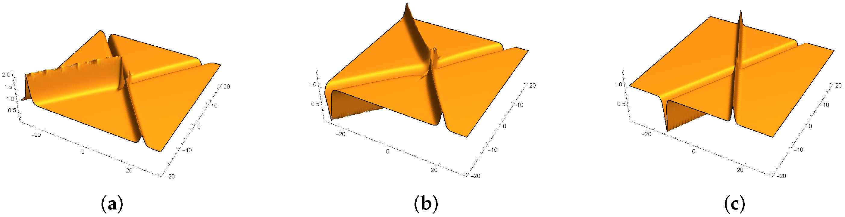
In any of these interactions, the interacting solitons can completely recover their individual shapes and velocities upon an interaction and have only the phase shifts for their envelopes. The Figure 1, Figure 2 and Figure 3 suggest that the solution (19a) under the condition (20) can describe the elastic soliton interactions on the cw background. The elastic interactions may occur between two antidark solitons, two dark solitons, or dark and antidark solitons. The existence of the antidark soliton or the dark soliton can be decided by the sign of c(z) [see Figure 1a–c]. Particularly taking ${\gamma }_{1I}=0$, the asymptotic solitons $(u_1^{-},u_1^{+})$ disappears as $z\to \pm \infty$, but $(u_2^{-},u_2^{+})$ still exists and represent antidark solitons for $c\left(z\right){\gamma }_{1R}<0$ or dark solitons for $c\left(z\right){\gamma }_{1R}>0$ [see Figure 4]. However, the solution (19a) in this degenerate case cannot be regarded as the conventional single soliton because there exists a phase shift between $u_2^{-}$ and $u_2^{+}$. Similarly, for the degenerate case $Im\left({\gamma }_1{\kappa }_1^2\right)=0$, one can find that only the pair of asymptotic solitons $(u_1^{-},u_1^{+})$ exists as $\left|z\right|\to \infty$ and there is also a phase shift between $u_1^{-}$ and $u_1^{+}$ [see Figure 5]. Associated with $c\left(z\right){\lambda }_{1I}{\gamma }_{1I}<0$ and $c\left(z\right){\lambda }_{1I}{\gamma }_{1I}>0$, $(u_1^{-},u_1^{+})$ can represent antidark solitons and dark solitons, respectively.

4. Rational Solutions of the PTNNLSESCS

In this section we construct the rational solutions of the PTNNLSESCS on the cw background. Equation (9) admits plane-wave solution $u=\rho e^{2i{\rho }^{2}z+i\varphi },\phi =0$. We take $c\left(z\right)=c_1\left(z\right)+i{c}_2\left(z\right),{\lambda }_1=i\rho$ to derive the rational solitons and rogue wave solutions. Inserting them into the Lax pair (10), by eigenvalue method we obtain

$$\begin{array}{cc}\hfill & f_1=\left(\begin{array}{c}{e}^{\frac{2i{\rho }^{2}z+i\varphi }{2}}\\ -i{e}^{-\frac{2i{\rho }^{2}z+i\varphi }{2}}\end{array}\right),\hfill \end{array}$$

(25a)

$$\begin{array}{cc}\hfill & g_1=\left(\begin{array}{c}\sqrt{2}i\rho (x+2z\rho +s_1)e^{\frac{2i{\rho }^{2}z+i\varphi }{2}}\\ \sqrt{2}(i+\rho (x+2z\rho +s_1))e^{-\frac{2i{\rho }^{2}z+i\varphi }{2}}\end{array}\right),\hfill \end{array}$$

(25b)

where $s_1$ is an arbitrary complex parameter.

Then, with substitution of (25) into the Darboux transformations (11), we obtain the first-order rational soliton solution as follows:

$$\begin{array}{cc}\hfill & u\left[1\right]=\rho e^{2i{\rho }^{2}z+i\varphi }\left[1-\frac{(2\xi +\sqrt{2}{K}_1-\sqrt{2}i)(2\eta +\sqrt{2}{K}_1^{*}-\sqrt{2}i)}{2\xi \eta +\sqrt{2}{K}_1^{*}\xi +\sqrt{2}{K}_1\eta +{\left|K_1\right|}^2+1}\right],\hfill \end{array}$$

(26a)

$$\begin{array}{cc}\hfill & {\phi }_1\left[1\right]=-\frac{\sqrt{\frac{i\rho c_2^{\prime }\left(z\right)}{-\sqrt{2}}}(2\eta +\sqrt{2}{K}_1^{*}-\sqrt{2}i)e^{\frac{2i{\rho }^{2}z+i\varphi }{2}}}{2\xi \eta +\sqrt{2}{K}_1^{*}\xi +\sqrt{2}{K}_1\eta +{\left|K_1\right|}^2+1},\hfill \end{array}$$

(26b)

$$\begin{array}{cc}\hfill & {\phi }_2\left[1\right]=\frac{-i\sqrt{\frac{i\rho c_2^{\prime }\left(z\right)}{-\sqrt{2}}}(2\eta +\sqrt{2}{K}_1^{*}+\sqrt{2}i)e^{-\frac{2i{\rho }^{2}z+i\varphi }{2}}}{2\xi \eta +\sqrt{2}{K}_1^{*}\xi +\sqrt{2}{K}_1\eta +{\left|K_1\right|}^2+1},\hfill \end{array}$$

(26c)

where $\xi =-i{c}_1\left(z\right)+c_2\left(z\right)+\sqrt{2}\rho (x+2z\rho ),\eta =i{c}_1\left(z\right)+c_2\left(z\right)+\sqrt{2}\rho (-x+2z\rho ),s_1=a+ib$ and $K_1=2\rho s_1+i$. The solution in Equation (26) has no singularity if and only if the following condition is satisfied:

$$\begin{array}{c}\hfill c_1\left(z\right)\ne \frac{2\rho b+1}{\sqrt{2}}.\end{array}$$

(27)

Under this condition, we perform an asymptotic analysis of the solution in Equation (26) so as to clarify the dynamical behavior underlying the solution.

(i) when $c_1\left(z\right)=0$. Firstly, we obtain the asymptotic expression of the solution in Equation (26) along the line $c_2\left(z\right)+\sqrt{2}\rho (x+2z\rho )\sim 0$ as $\left|z\right|\to \infty$ as follows:

$$\begin{array}{cc}\hfill & u\left[1\right]\to u^I=\rho e^{2i{\rho }^{2}z+i\varphi }\left[1-\frac{2(\sqrt{2}\xi +K_1-i)}{\sqrt{2}\xi +K_1}\right],\hfill \end{array}$$

(28a)

$$\begin{array}{cc}\hfill & {\left|u\left[1\right]\right|}^2\to {\left|u^I\right|}^2={\rho }^2\left[1-\frac{8\rho Im\left(s_1\right)}{|\sqrt{2}\xi +K_1{|}^2}\right],\hfill \end{array}$$

(28b)

$$\begin{array}{cc}\hfill & {\phi }_1\left[1\right]\to {\phi }_1^I=\frac{-\sqrt{-\sqrt{2}i\rho c_2^{\prime }\left(z\right)}{e}^{\frac{2i{\rho }^{2}z+i\varphi }{2}}}{\sqrt{2}\xi +K_1},\hfill \end{array}$$

(29a)

$$\begin{array}{cc}\hfill & |{\phi }_1{\left[1\right]|}^2\to {\left|{\phi }_1^I\right|}^2=\frac{\sqrt{2}\rho \left|c_2^{\prime }\left(z\right)\right|}{|\sqrt{2}\xi +K_1{|}^2},\hfill \end{array}$$

(29b)

$$\begin{array}{cc}\hfill & {\phi }_2\left[1\right]\to {\phi }_2^{II}=\frac{-i\sqrt{-\sqrt{2}i\rho c_2^{\prime }\left(z\right)}{e}^{-\frac{2i{\rho }^{2}z+i\varphi }{2}}}{\sqrt{2}\xi +K_1},\hfill \end{array}$$

(30a)

$$\begin{array}{cc}\hfill & |{\phi }_2{\left[1\right]|}^2\to {\left|{\phi }_2^{II}\right|}^2=\frac{\sqrt{2}\rho \left|c_2^{\prime }\left(z\right)\right|}{|\sqrt{2}\xi +K_1{|}^2}.\hfill \end{array}$$

(30b)

Secondly, we derive the asymptotic expression of the solution in Equation (26) along the line $c_2\left(z\right)+\sqrt{2}\rho (-x+2z\rho )\sim 0$ as $\left|z\right|\to \infty$ as follows:

$$\begin{array}{cc}\hfill & u\left[1\right]\to u^{II}=\rho e^{2i{\rho }^{2}z+i\varphi }\left[1-\frac{2(\sqrt{2}\eta +K_1^{*}-i)}{\sqrt{2}\eta +K_1^{*}}\right],\hfill \end{array}$$

(31a)

$$\begin{array}{cc}\hfill & {\left|u\left[1\right]\right|}^2\to {\left|u^{II}\right|}^2={\rho }^2\left[1+\frac{8(1+\rho Im\left(s_1\right))}{|\sqrt{2}\eta +K_1^{*}{|}^2}\right],\hfill \end{array}$$

(31b)

$$\begin{array}{cc}\hfill & {\phi }_1\left[1\right]=-\frac{\sqrt{\frac{i\rho c_2^{\prime }\left(z\right)}{-\sqrt{2}}}(2\eta +\sqrt{2}{K}_1^{*}-\sqrt{2}i)e^{\frac{2i{\rho }^{2}z+i\varphi }{2}}}{2\xi \eta +\sqrt{2}{K}_1^{*}\xi +\sqrt{2}{K}_1\eta +{\left|K_1\right|}^2+1}\to 0,\hfill \end{array}$$

(32)

$$\begin{array}{cc}\hfill & {\phi }_2\left[1\right]=\frac{-i\sqrt{\frac{i\rho c_2^{\prime }\left(z\right)}{-\sqrt{2}}}(2\eta +\sqrt{2}{K}_1^{*}+\sqrt{2}i)e^{-\frac{2i{\rho }^{2}z+i\varphi }{2}}}{2\xi \eta +\sqrt{2}{K}_1^{*}\xi +\sqrt{2}{K}_1\eta +{\left|K_1\right|}^2+1}\to 0.\hfill \end{array}$$

(33)

The above asymptotic analysis shows three different types of elastic interactions. The associated parametric conditions are given in

Table 2. Asymptotic patterns of the solution (26a) under different parametric conditions.

	Parametric Conditions	Asymptotic Soliton ${\mathit{u}}^{\mathit{I}}$	Asymptotic Soliton ${\mathit{u}}^{\mathit{II}}$
	$Im\left(s_1\right)<0,1+\rho Im\left(s_1\right)>0$	RAD soliton	RAD soliton
	$Im\left(s_1\right)<0,1+\rho Im\left(s_1\right)<0$	RAD soliton	RD soliton
	$Im\left(s_1\right)>0,1+\rho Im\left(s_1\right)>0$	RD soliton	RAD soliton
	$Im\left(s_1\right)=0$	disappear	RAD soliton
	$1+\rho Im\left(s_1\right)=0$	RAD soliton	disappear

. For the cases $Im\left(s_1\right)>0$ and $Im\left(s_1\right)<0$, the intensity $|u^I{|}^2$ can respectively exhibit the rational dark (RD) soliton beneath the cw background $u=\rho e^{2i{\rho }^{2}z+i\varphi },\phi =0$ and the rational antidark (RAD) soliton on top of the same background, and the valley and peak are both localized along the line $\sqrt{2}{c}_2\left(z\right)+2\rho (x+2z\rho )+Re\left(K_1\right)=0$. The intensity $|u_1^{II}{|}^2$ display the RD and RAD soliton profiles which are associated with $1+\rho Im\left(s_1\right)<0$ and $1+\rho Im\left(s_1\right)>0$ respectively. In this case, both the RD and RAD solitons are localized along the line $\sqrt{2}{c}_2\left(z\right)+2\rho (-x+2z\rho )+Re\left(K_1\right)=0$. In particular, for the degenerate case $Im\left(s_1\right)=0$, the asymptotic soliton $u^I$ disappear as $z\to \pm \infty$. Similarly, for the degenerate case $1+\rho Im\left(s_1\right)=0$, the only surviving asymptotic soliton is $u^I$.

The heights of the RAD soliton or the depth of the RD soliton from the cw background for $|u^I|$ and $|u^{II}|$, that is $A_1=\frac{8{\rho }^{3}Im\left(s_1\right)}{2\rho Im\left(s_1\right)+1}$ and $A_2=\frac{8{\rho }^2(1+\rho Im\left(s_1\right))}{2\rho Im\left(s_1\right)+1}$, respectively. The velocities of the RD and RAD solitons from the cw background for $|u^I|$ and $|u^{II}|$, that is $v_1=-2\rho -\frac{c_2^{\prime }\left(z\right)}{\sqrt{2}\rho }$ and $v_2=2\rho +\frac{c_2^{\prime }\left(z\right)}{\sqrt{2}\rho }$, respectively.

The asymptotic analysis implies that Equation (26) can describe the elastic interactions of rational solitons as two interacting solitons retain their individual shapes, intensities and velocities as $z\to \infty$. However, different from the standard elastic interaction in the PTNNLSESCS, each soliton experiences no phase shift upon the interaction.

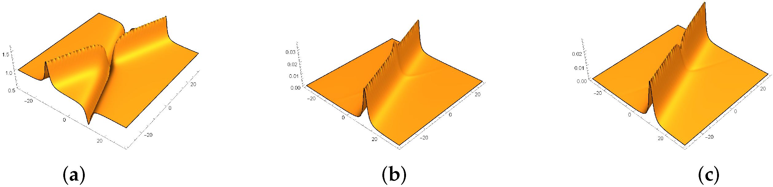
In general, Equation (26) exhibits three different types of elastic interactions between two rational solitons on a cw background, as shown in Figure 6, Figure 7, Figure 8, Figure 9, Figure 10 and Figure 11. More specifically, with $Im\left(s_1\right)<0$ and $1+\rho Im\left(s_1\right)>0$, the asymptotic soliton $u^I$ and $u^{II}$ both displays RAD solitons profile [see Figure 6a]. With $Im\left(s_1\right)<0$ and $1+\rho Im\left(s_1\right)<0$, the asymptotic soliton $u^I$ and $u^{II}$ displays RAD and RD solitons profile [see Figure 7a]. With $Im\left(s_1\right)>0$ and $1+\rho Im\left(s_1\right)>0$, the asymptotic soliton $u^I$ and $u^{II}$ displays RD and RAD solitons profile [see Figure 8a]. The function c(z) of the solutions (26) can change the shape of the RAD or RD [see Figure 9, Figure 10 and Figure 11]. The solution of ${\phi }_1\left[1\right]$ and ${\phi }_2\left[1\right]$ always diplay RAD soliton solution along the line $c_2\left(z\right)+\sqrt{2}\rho (x+2z\rho )=0$ as $\left|z\right|\to \infty$ and has a constant height as $c_2\left(z\right)=z$ [see Figure 6b,c], but the height change as $c_2\left(z\right)=z^2$ [see Figure 9b,c]. The solution of ${\phi }_1\left[1\right]$ and ${\phi }_2\left[1\right]$ disappear along the line $c_2\left(z\right)+\sqrt{2}\rho (-x+2z\rho )=0$ as $\left|z\right|\to \infty$.

In particular, with $Im\left(s_1\right)=0$ the asymptotic soliton $u^I$ disappear as $z\to \pm \infty$ while $u^{II}$ displays a RAD soliton profile [see Figure 12]. Similarly, for the degenerate case $1+\rho Im\left(s_1\right)=0$, the only surviving asymptotic soliton is $u^I$ and it takes the shape of the RAD type [see Figure 13]. In either of the two degenerate cases, one asymptotic soliton disappears in the far-field region, but it still affects the other one in the near-field region, that is, the surviving soliton is segmented into two pieces at some finite value of z. Therefore, such two degenerate cases of the solution in Equation (26a) cannot be simply regarded as the conventional single soliton.

(ii) when $c_1\left(z\right)\ne 0$, Equation (26) can be written as follows:

$$\begin{array}{cc}\hfill & u\left[1\right]=\rho e^{2i{\rho }^{2}z+i\varphi }(-1+\frac{G_1}{H_1+iH}),\hfill \end{array}$$

(34a)

$$\begin{array}{cc}\hfill & {\phi }_1\left[1\right]=-\frac{G_2}{H_1+iH},\hfill \end{array}$$

(34b)

$$\begin{array}{cc}\hfill & {\phi }_2\left[1\right]=\frac{G_3}{H_1+iH},\hfill \end{array}$$

(34c)

where

$$\begin{array}{cc}\hfill & G_1=2(2\sqrt{2}i(c_2\left(z\right)+2\sqrt{2}{\rho }^{2}z)+4i\rho a+2),\hfill \\ \hfill & G_2=\sqrt{-\sqrt{2}i\rho c_2^{\prime }\left(z\right)}(\sqrt{2}i{c}_1\left(z\right)+\sqrt{2}{c}_2\left(z\right)+2\rho (-x+2z\rho )+2(a-ib)-2i)e^{\frac{2i{\rho }^{2}z+i\varphi }{2}},\hfill \\ \hfill & G_3=-i\sqrt{-\sqrt{2}i\rho c_2^{\prime }\left(z\right)}(\sqrt{2}i{c}_1\left(z\right)+\sqrt{2}{c}_2\left(z\right)+2\rho (-x+2z\rho )+2(a-ib))e^{-\frac{2i{\rho }^{2}z+i\varphi }{2}},\hfill \\ \hfill & H_1=2{(\sqrt{2}\rho a+c_2\left(z\right)+2\sqrt{2}{\rho }^{2}z)}^2+{(\sqrt{2}\rho b-c_1\left(z\right))}^2+{(\sqrt{2}\rho b+\sqrt{2}-c_1)}^2-4{\rho }^2{x}^2,\hfill \\ \hfill & H_2=-4\rho x(2\rho b-\sqrt{2}{c}_1\left(z\right)+1).\hfill \end{array}$$

We can see that the solution of (34a) tends to background in the z direction as $\left|z\right|\to \infty$ because the denominator containing $z^2$ and ${\left(c_2\left(z\right)\right)}^2$ has higher exponential than the molecule containing z and $c_2\left(z\right)$. The solution of (34a) tends to background in the x direction as $\left|x\right|\to \infty$ because the denominator contains $x^2$ and x, but the molecule does not contain the x. So the solution of (34a) would tend to background in all direction, which means that we get the rogue wave solution as shown in Figure 14a. The solution of (34b) tends to background in the z direction as $\left|z\right|\to \infty$ because the denominator containing $z^2$, ${\left(c_1\left(z\right)\right)}^2$ and ${\left(c_2\left(z\right)\right)}^2$ has higher exponential than the molecule containing z, $c_1\left(z\right)$ and $c_2\left(z\right)$. The solution of (34b) tends to background in the x direction as $\left|x\right|\to \infty$ because the denominator contains $x^2$ and x, but the molecule only contains the x. So the solution of (34b) would tend to background in all direction, which means that we get the rogue wave solution as shown in Figure 14b. The solution of (34c) has the same reason as the solution of (34b) as shown in Figure 14c.

5. Conclusions

In this paper, we have studied the nonlinear localized wave on the cw background for the PTNNLSESCS. The generalized Darboux transformation for the PTNNLSESCS is derived. We have derived the nonsingular first-order soliton solution, the first-order rational soliton solution and rogue wave solution from a cw solution by the generalized Darboux transformation. We have revealed the elastic antidark-antidark soliton, antidark-dark soliton, and dark-dark soliton interactions, in which there is a phase shift for interacting solitons. we have also revealed the elastic RAD-RAD and RAD-RD soliton interactions, in which there is no phase shift for interacting solitons. Meanwhile, we have discussed the degenerate case in which only one soliton remains.

References

1. Bender, C.M.; Boettcher, S. Real Spectra in Non-Hermitian Hamiltonians Having PT-Symmetry. Phys. Rev. Lett. 1998, 80, 5243. [Google Scholar] [CrossRef] [Green Version]
2. Bender, C.M.; Brody, D.C.; Jones, H.F.; Meister, B.K. Faster than Hermitian Quantum Mechanics. Phys. Rev. Lett. 2007, 98, 040403. [Google Scholar] [CrossRef] [PubMed] [Green Version]
3. El-Ganainy, R.; Makris, K.G.; Christodoulides, D.N.; Musslimani, Z.H. Theory of coupled optical PT-symmetric structures. Opt. Lett. 2007, 32, 2632–2634. [Google Scholar] [CrossRef]
4. Makris, K.G.; El-Ganainy, R.; Christodoulides, D.N.; Musslimani, Z.H. Beam Dynamics in PT Symmetric Optical Lattices. Phys. Rev. Lett. 2008, 100, 103904. [Google Scholar] [CrossRef]
5. Guo, A.; Salamo, G.J.; Duchesne, D.; Morandotti, R.; Volatier-Ravat, M.; Aimez, V.; Siviloglou, G.A.; Christodoulides, D.N. Observation of PT-Symmetry Breaking in Complex Optical Potentials. Phys. Rev. Lett. 2009, 103, 093902. [Google Scholar] [CrossRef] [PubMed] [Green Version]
6. He, Y.J.; Zhu, X.; Mihalache, D.; Liu, J.L.; Chen, Z.X. Lattice solitons in PT-symmetric mixed linear-nonlinear optical lattices. Phys. Rev. A 2012, 85, 013831. [Google Scholar] [CrossRef]
7. Ablowitz, M.J.; Musslimani, Z.H. Integrable Nonlocal Nonlinear Schrödinger Equation. Phys. Rev. Lett. 2013, 110, 064105. [Google Scholar] [CrossRef] [Green Version]
8. Li, M.; Xu, T. Dark and antidark soliton interactions in the nonlocal nonlinear Schrödinger equation with the self-induced parity-time-symmetric potential. Phys. Rev. E 2015, 91, 033202. [Google Scholar] [CrossRef]
9. Li, M.; Xu, T.; Meng, D.X. Rational Solitons in the Parity-Time-Symmetric Nonlocal Nonlinear Schrödinger Model. J. Phys. Soc. Jpn. 2016, 85, 124001. [Google Scholar] [CrossRef] [Green Version]
10. Dai, C.Q.; Huang, W.H. Multi-rogue wave and multi-breather solutions in PT-symmetric coupled waveguides. Appl. Math. Lett. 2014, 32, 35–40. [Google Scholar] [CrossRef]
11. Sarma, A.K.; Miri, M.A.; Musslimani, Z.H.; Christodoulides, D.N. Continuous and discrete Schrödinger systems with parity-time-symmetric nonlinearities. Phys. Rev. E 2014, 89, 052918. [Google Scholar] [CrossRef] [PubMed] [Green Version]
12. Wen, X.Y.; Yan, Z.Y.; Yang, Y.Q. Dynamics of higher-order rational solitons for the nonlocal nonlinear Schrödinger equation with the self-induced parity-time-symmetric potential. Chaos 2016, 6, 063123. [Google Scholar] [CrossRef] [PubMed] [Green Version]
13. Zhou, Z.X. Darboux transformations and global explicit solutions for nonlocal Davey-Stewartson I equation. arXiv 2018, arXiv:1612.05689. [Google Scholar] [CrossRef]
14. Xu, T.; Li, M.; Huang, Y.H.; Chen, Y.; Yu, C. Nonsingular localized wave solutions for the nonlocal Davey-Stewartson I equation with zero background. Mod. Phys. Lett. B 2017, 35, 1750338. [Google Scholar] [CrossRef]
15. Li, M.; Shui, J.J.; Xu, T. Generation mechanism of rogue waves for the discrete nonlinear Schrödinger equation. Appl. Math. Lett. 2018, 83, 110–115. [Google Scholar] [CrossRef]
16. Chen, K.; Deng, X.; Lou, S.Y.; Zhang, D.J. Solutions of local and nonlocal equations reduced from the AKNS hierarchy. Stud. Appl. Math. 2018, 141, 113–141. [Google Scholar] [CrossRef]
17. Duanmu, M.; Li, K.; Horne, R.L.; Kevrekidis, P.G.; Whitaker, N. Linear and nonlinear parity-time-symmetric oligomers: A dynamical systems analysis. Philos. Trans. R. Soc. A 2013, 1989, 20120171. [Google Scholar] [CrossRef] [Green Version]
18. Zhang, Y.J.; Yang, C.Y.; Yu, W.T.; Mirzazadeh, M.; Zhou, Q.; Liu, W.J. Interactions of vector anti-dark solitons for the coupled nonlinear Schrödinger equation in inhomogeneous fibers. Nonlinear Dyn. 2018, 94, 1351–1360. [Google Scholar] [CrossRef]
19. Zhang, H.Q.; Zhai, B.G.; Wang, X.L. Dark and antidark soliton solutions in the modified nonlinear Schrödinger equation with distributed coefficients in inhomogeneous fibers. Phys. Scr. 2012, 85, 015006. [Google Scholar] [CrossRef]
20. Zhang, X.Z.; Zhang, Y.F. Some invariant solutions and conservation laws of a type of long-water wave system. Adv. Differ. Equ. 2019, 2019, 496. [Google Scholar] [CrossRef] [Green Version]
21. El-Nabulsi, R.A. Non-standard higher-order G-strand partial differential equations on matrix Lie algebra. J. Niger. Math. Soc. 2017, 36, 101–112. [Google Scholar]
22. Camassa, R.; Holm, D.D. An integrable shallow water equation with peaked solitons. Phys. Rev. Lett. 1993, 71, 1661. [Google Scholar] [CrossRef] [PubMed] [Green Version]
23. Novikov, V. Generalizations of the Camassa-Holm equation. J. Phys. A Math. Theor. 2009, 42, 342002. [Google Scholar] [CrossRef]
24. Qu, C.Z.; Liu, X.C.; Liu, Y. Stability of peakons for an integrable modified Camassa-Holm equation with cubic nonliearity. Commun. Math. Phys. 2013, 322, 967–997. [Google Scholar] [CrossRef]
25. Lou, S.Y.; Qiao, Z.J. Alice-Bob Peakon Systems. Chin. Phys. Lett. 2017, 34, 100201. [Google Scholar]
26. Claude, C.; Latifi, A.; Leon, J. Nonlinear resonant scattering and plasma instability: An integrable model. J. Math. Phys. 1991, 32, 3321. [Google Scholar] [CrossRef]
27. Shao, Y.J.; Zeng, Y.B. The solutions of the NLS equations with self-consistent sources. J. Phys. A Math. Gen. 2005, 38, 2441–2467. [Google Scholar] [CrossRef]
28. Meng, G.Q.; Qin, J.L.; Yu, G.L. Breather and rogue wave solutions for a nonlinear Schrödinger-type systems in plasmas. Nonlinear Dyn. 2015, 81, 739. [Google Scholar] [CrossRef]
29. Mel’nikov, V.K. On equations for wave intections. Lett. Math. Phys. 1983, 7, 129–136. [Google Scholar] [CrossRef]
30. Zeng, Y.B.; Shao, Y.J.; Ma, W.X. Integral-Type Darboux Transformation for the mKdV Hierarchy with Self-Consistent Sources. Commun. Theor. Phys. 2002, 38, 641–648. [Google Scholar]
31. Huang, Y.H.; Yao, Y.Q.; Zeng, Y.B. On Camassa-Holm Equation with Self-Consistent Sources and Its Solutions. Commun. Theor. Phys. 2010, 53, 403–412. [Google Scholar]
32. Yao, Y.Q.; Huang, Y.H.; Zeng, Y.B. The Qiao-Liu Equation with Self-Consistent Sources and Its Solutions. Commun. Theor. Phys. 2012, 57, 909–913. [Google Scholar] [CrossRef]
Figure 1. Elastic interactions via the solution (19a): (a) dark and antidark solitons with ρ = 1 , λ 1 = 0.1 i , c ( z ) = z and γ 1 = 0.4 0.5 i ; (b) two dark solitons with ρ = 1 , λ 1 = 0.1 i , c ( z ) = z 2 and γ 1 = 0.4 0.5 i ; (c) two dark solitons with ρ = 1 , λ 1 = 0.1 i , c ( z ) = e z and γ 1 = 0.4 0.5 i .
Mathematics 08 01099 g001
Figure 2. Elastic interactions via the solution (19a): (a) dark and antidark solitons with ρ = 1 , λ 1 = 0.4 i , c ( z ) = z and γ 1 = 2 0.6 i ; (b) two antidark solitons with ρ = 1 , λ 1 = 0.4 i , c ( z ) = z 2 and γ 1 = 2 0.6 i ; (c) two antidark solitons with ρ = 1 , λ 1 = 0.4 i , c ( z ) = e z and γ 1 = 2 0.6 i .
Mathematics 08 01099 g002
Figure 3. Elastic interactions via the solution (19a): (a) dark and antidark solitons with ρ = 1 , λ 1 = 0.4 i , c ( z ) = z and γ 1 = 2 0.5 i ; (b) dark and antidark solitons with ρ = 1 , λ 1 = 0.4 i , c ( z ) = z 2 and γ 1 = 2 0.5 i ; (c) dark and antidark solitons with ρ = 1 , λ 1 = 0.4 i , c ( z ) = e z and γ 1 = 2 0.5 i .
Mathematics 08 01099 g003
Figure 4. Degenerate two-solution interaction via the solution (19a): (a) dark and antidark soliton with a phase shift between two soliton segments as z ± , where ρ = 1 , λ 1 = 0.5 i , c ( z ) = z and γ 1 = 1 ; (b) antidark soliton with a phase shift between two soliton segments as z ± , where ρ = 1 , λ 1 = 0.5 i , c ( z ) = z 2 and γ 1 = 1 ; (c) antidark soliton with a phase shift between two soliton segments as z ± , where ρ = 1 , λ 1 = 0.5 i , c ( z ) = e z and γ 1 = 1 .
Mathematics 08 01099 g004
Figure 5. Degenerate two-solution interaction via the solution (19a): (a) dark and antidark soliton with a phase shift between two soliton segments as z ± , where ρ = 1 , λ 1 = 0.5 i , c ( z ) = z and γ 1 = 3 3 + i ; (b) dark soliton with a phase shift between two soliton segments as z ± , where ρ = 1 , λ 1 = 0.5 i , c ( z ) = z 2 and γ 1 = 3 3 + i ; (c) dark soliton with a phase shift between two soliton segments as z ± , where ρ = 1 , λ 1 = 0.5 i , c ( z ) = e z and γ 1 = 3 3 + i .
Mathematics 08 01099 g005
Figure 6. (ac) are the first-order rational soliton solutions via Equations (26a)–(26c) with ρ = 0.5 , ϕ = 0 , c 1 ( z ) = 0 , c 2 ( z ) = z and γ 1 = 1 0.1 i , respectively.
Mathematics 08 01099 g006
Figure 7. (ac) are the first-order rational soliton solution via Equations (26a)–(26c) with ρ = 1 , ϕ = 0 , c 1 ( z ) = 0 , c 2 ( z ) = z and γ 1 = 1 3 i , respectively.
Mathematics 08 01099 g007
Figure 8. (ac) are the first-order rational soliton solution via Equations (26a)–(26c) with ρ = 1 , ϕ = 0 , c 1 ( z ) = 0 , c 2 ( z ) = z and γ 1 = 1 + 3 i , respectively.
Mathematics 08 01099 g008
Figure 9. (ac) are the first-order rational soliton solution via Equations (26a)–(26c) with ρ = 1 , ϕ = 0 , c 1 ( z ) = 0 , c 2 ( z ) = z 2 and γ 1 = 1 0.1 i , respectively.
Mathematics 08 01099 g009
Figure 10. (ac) are the first-order rational soliton solution via Equations (26a)–(26c) with ρ = 1 , ϕ = 0 , c 1 ( z ) = 0 , c 2 ( z ) = z 2 and γ 1 = 1 3 i , respectively.
Mathematics 08 01099 g010
Figure 11. (ac) are the first-order rational soliton solution via Equations (26a)–(26c) with ρ = 1 , ϕ = 0 , c 1 ( z ) = 0 , c 2 ( z ) = z 2 and γ 1 = 1 + 3 i , respectively.
Mathematics 08 01099 g011
Figure 12. Degenerate two-solution interaction via the solution in Equation (26a): (a) antidark soliton as z ± , where ρ = 0.5 , ϕ = 0 , c 1 ( z ) = 0 , c 2 ( z ) = z and γ 1 = 1 ; (b) antidark soliton as z ± , where ρ = 0.5 , ϕ = 0 , c 1 ( z ) = 0 , c 2 ( z ) = z 2 and γ 1 = 1 .
Mathematics 08 01099 g012
Figure 13. Degenerate two-solution interaction via the solution Equation (26a): (a) antidark soliton as z ± , where ρ = 0.5 , ϕ = 0 , c ( z ) = z and γ 1 = 1 2 i ; (b) antidark soliton as z ± , where ρ = 0.5 , c ( z ) = z 2 and γ 1 = 1 2 i .
Mathematics 08 01099 g013
Figure 14. (ac) are the rogue wave solution via Equations (26a)–(26c) with ρ = 1 , ϕ = 0 , c 1 ( z ) = z 2 + 3 2 , c 2 ( z ) = z 2 and γ 1 = 1 + 2 i , respectively.
Mathematics 08 01099 g014