Multi-Objective Environmental Economic Dispatch of an Electricity System Considering Integrated Natural Gas Units and Variable Renewable Energy Sources

 ,
,  ,
,  and
and 
Abstract
:1. Introduction
- Formulation of the MOEED problem considering thermal, solar, wind, hydropower, and natural gas units.
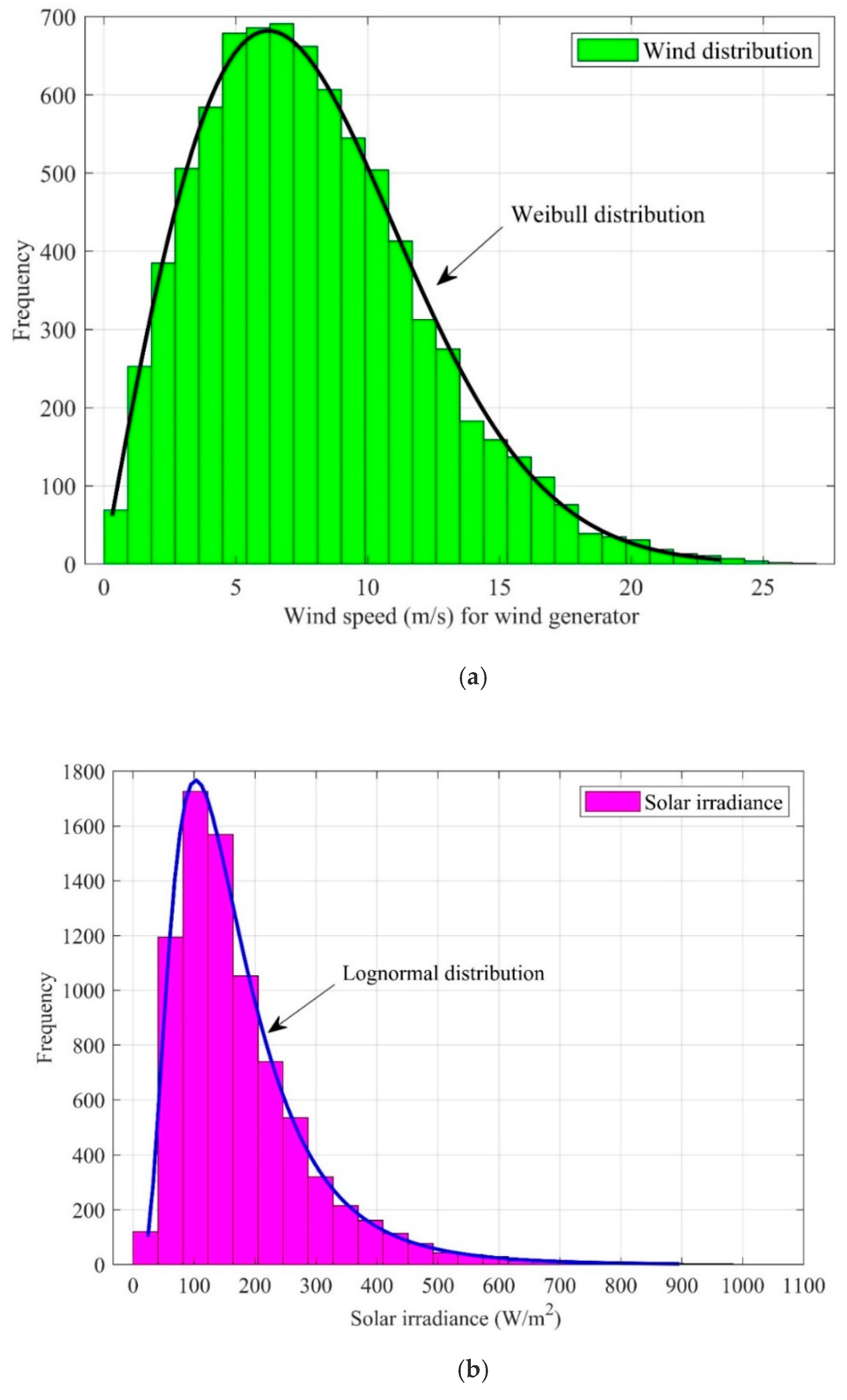
- Stochastic analysis of VRESs used has been presented using the most proper PDFs.
- All system constraints like security, equality, and inequality power flow conditions, POZs limits, and NG constraints are considered in the formulated MOEED problem.
- MOO techniques such as MOHHOA and MOFPA are employed to solve the MOEED problem.
- A comparative analysis of the solutions obtained by the three optimization techniques is proposed.
- TOPSIS is used to obtain the best compromise solution to the MOEED problem.
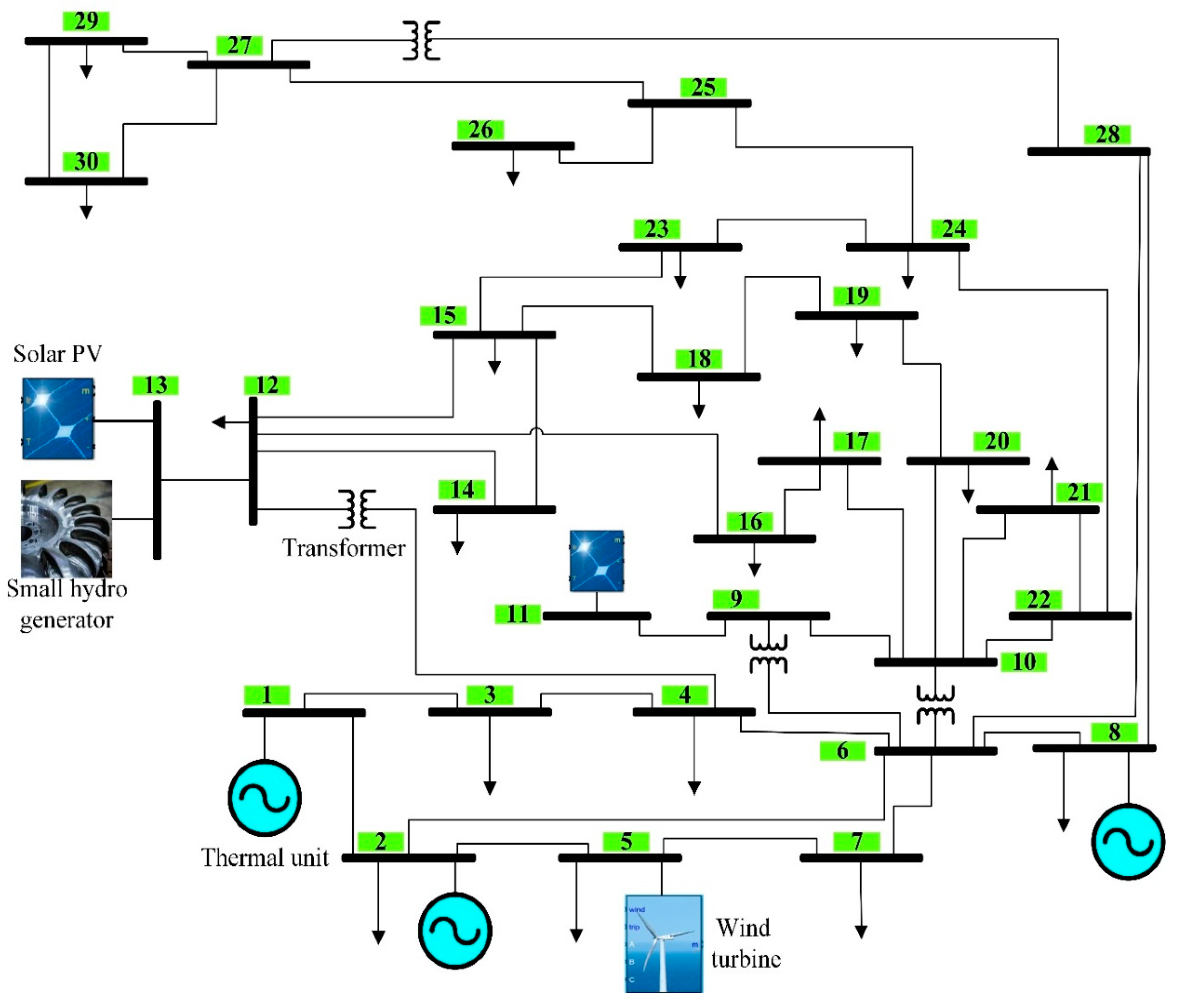
2. System Studied
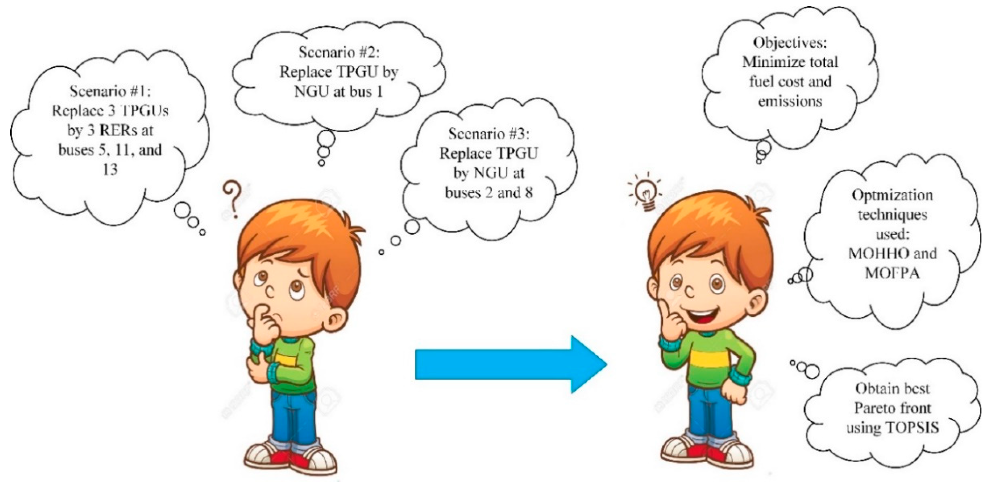
- Scenario I: Using three TPGUs and three VRESs [24].
- Scenario II: Replacing the fuel of TPGU at bus 1 into NGU.
- Scenario III: Replacing the fuel of TPGUs at buses 2 and 8 into NGUs.
3. Formulation of the Multi-Objective Function
3.1. Objective Functions
3.1.1. Total Fuel Costs
Fuel Cost Analysis of Thermal Power Generation Units (TPGUs)
Fuel Cost Analysis of Variable Renewable Energy Sources (VRESs)
A. Cost Calculation of Wind Plants
B. Cost Calculation of the Solar Plant
C. Cost Calculation of the Photovoltaic and Small Hydropower (PVSH) Plant
Fuel Cost Analysis of Natural Gas Units (NGUs)
3.1.2. Emission Levels
Emission Analysis of TPGUs
Emission Analysis of NGUs
3.2. Constraints
3.2.1. Power Balance Constraints
3.2.2. Rating Limitations
Active and Reactive Powers Limits
Prohibited Operating Zones Limits
Security Constraints
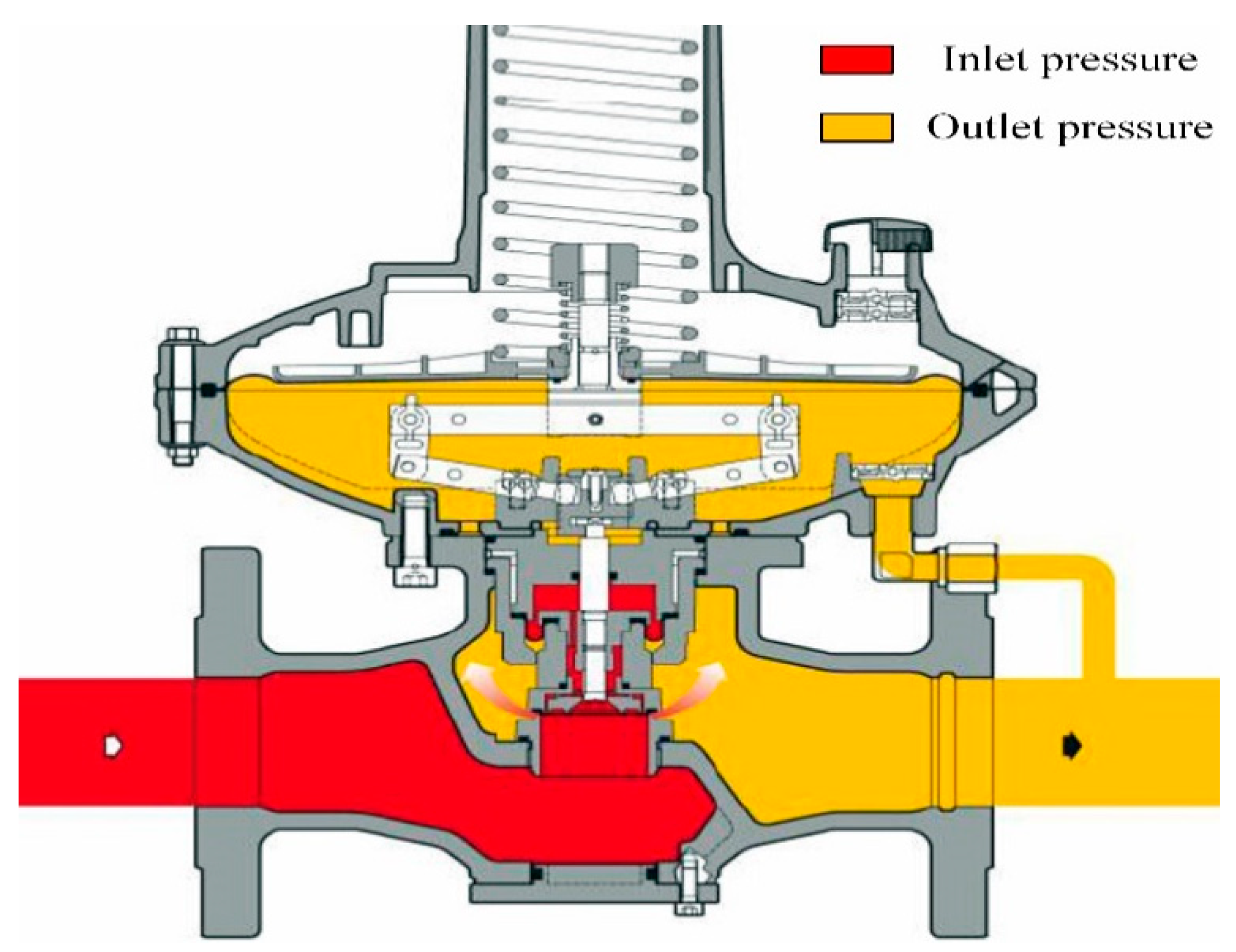
3.2.3. Natural Gas Limits
3.3. Multi-Objective Optimization Techniques
- Step 1: Solutions are arranged in each objective domain.
- Step 2: Crowded distances of the first solution and the last solution in the rank are selected as to infinity.
- Step 3: For each of the other solutions, the crowded distance will be calculated in Equation (55):where M, i, and j represent the objectives number, the number of the solution, and the total number of solutions in the set Fr, respectively. and represent the mth objective functions of solution number (i + 1) and (i − 1) in the set Fr, respectively. and represent the minimum and maximum values of the mth objective function in the set Fr, respectively.
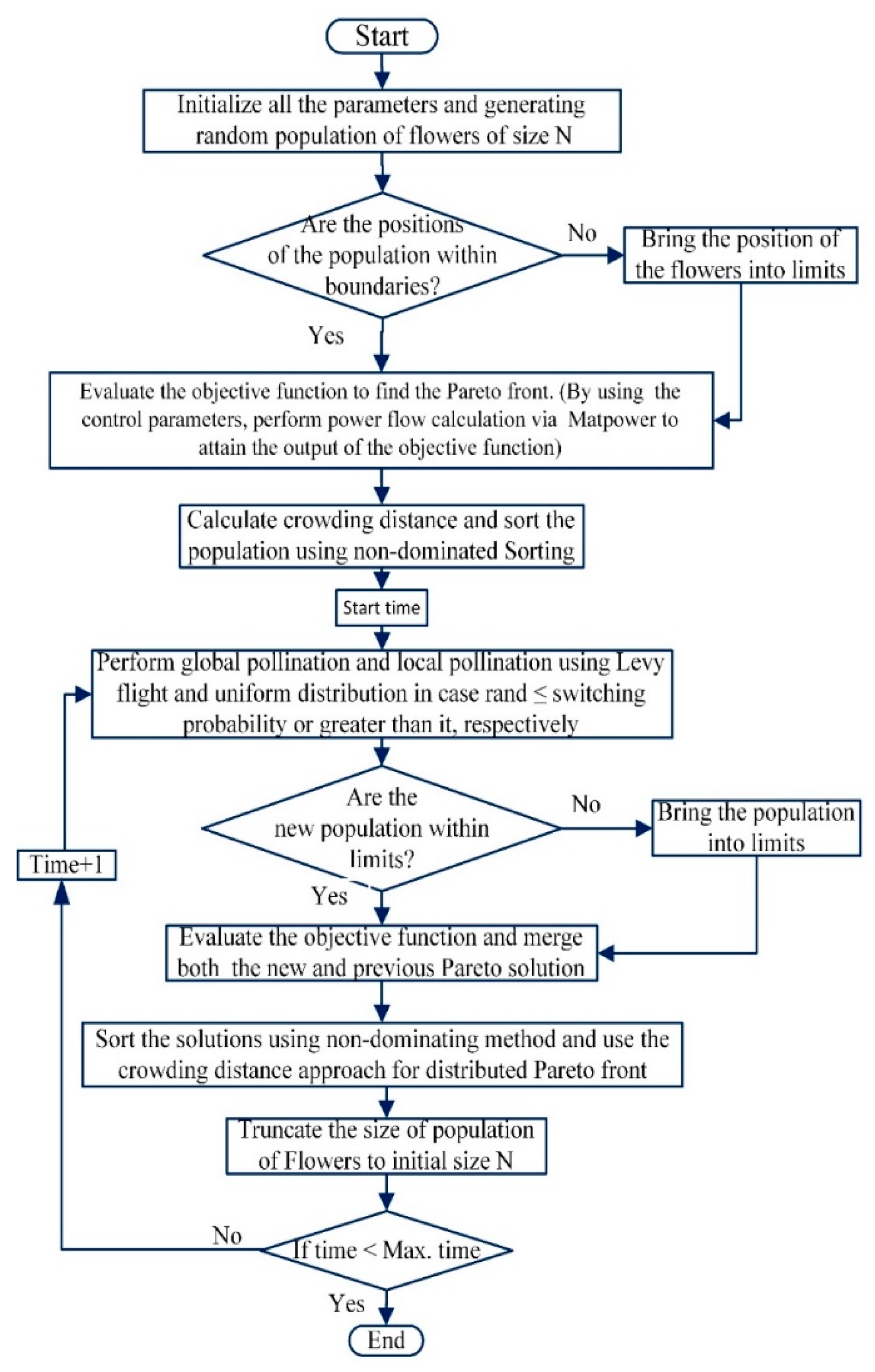
3.3.1. Multi-Objective Flower Pollination Algorithm (MOFPA)
- Rule 1:
- Global pollinators fly large distances for pollination, and are close to Levy flights in their movement.
- Rule 2:
- Local pollination is achieved using abiotic self-pollination.
- Rule 3:
- Local pollination occurs among the same flowers or flowers of the same species.
- Rule 4:
- A switch probability () lying in the interval (0,1) decides whether the pollination of a flower is local or global. The algorithm can be formulated as:
- (1)
- Global pollination is implemented when a uniform production arbitrary value , illustrated in Equation (56), to sequentially change the location of the ith flower utilizing its spacing from the best flower .where denotes the Levy flight attitudes of the pollinators. This follows that the distribution of Levy reflects the intensity of the pollination. To control the size of the step, a scaling factor ( is chosen.
- (2)
- In the FPA technique, the local pollination will be performed to use a uniform distribution random value that lies from 0 to 1 to regulate the mutation in the ith flower.
| Algorithm 1: Multi-objective flower pollination algorithm (MOFPA) pseudo code |
 |
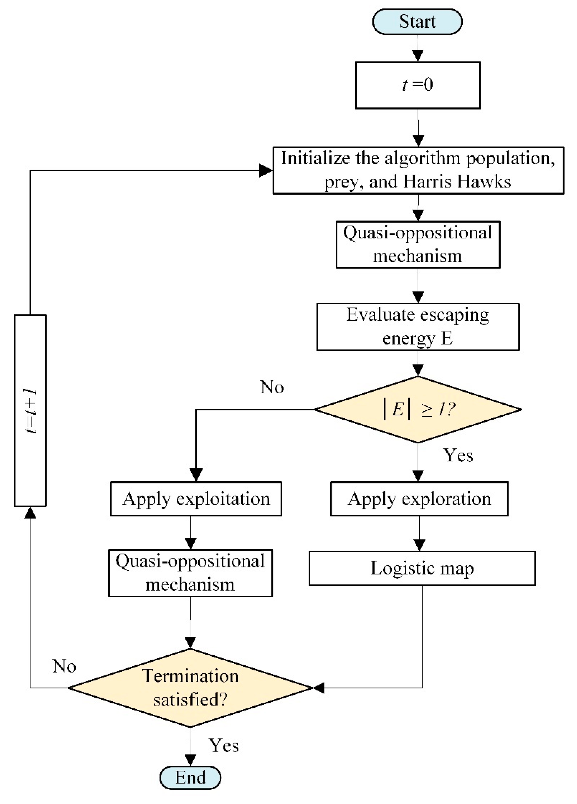
3.3.2. Multi-Objective Harris Hawks Optimization (MOHHO)
A. Soft Besiege
B. Hard Besiege
C. Soft Besiege with Progressive Rapid Dive
- Hard besiege with progressive quick dive.
- Hard besiege with progressive quick dive is suitable if r≺ 0 and ≺ 0. In that event, the victim does not have sufficient energy to escape properly. This case is expressed in Equation (71):
| Algorithm 2: MOHHO pseudo code. |
 |
3.3.3. A Technique for Order Preference by Similarity to Ideal Solution (TOPSIS)
- Step 1:
- Determine a decision matrix S (composed of a set of non-dominant solutions of the Pareto solutions). The value is an indication for the performance rating of the ith alternative concerning the jth function. Let, be the relative weight vector about the objectives, satisfying .
- Step 2:
- Determine the normalized value by applying Equation (72), i.e., by normalizing the decision matrix:
- Step 3:
- Determine using Equation (73) that denotes the weighted normalized decision matrix.
- Step 4:
- Get and using Equations (74) and (75):
- Step 5:
- Using the n-dimensional Euclidean distance, determine the separation measures by Equations (76) and (77):
- Step 6:
- Determine the relative closeness (RC) or performance index to the ideal solution, which has been formulated as in Equation (78):
- Step 7:
- The preference order is to be ranked, so that the best compromise solution is considered as the solution with the greatest RC to the ideal solution.
4. Simulation Results and Comparative Analysis
- Scenario I: Using three TPGUs and three VRESs [24].
- Scenario II: Replacing the fuel of TPGU at bus 1 into NGU.
- Scenario III: Replacing the fuel of TPGUs at buses 2 and 8 into NGUs.
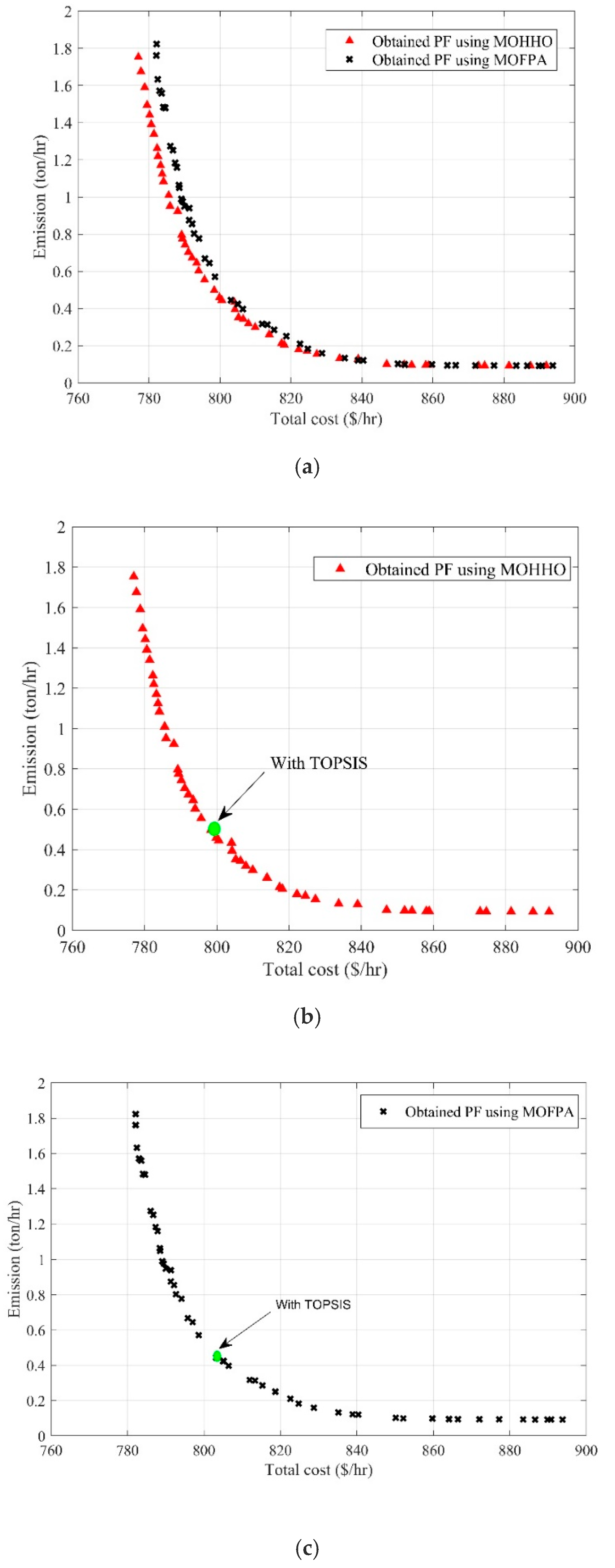
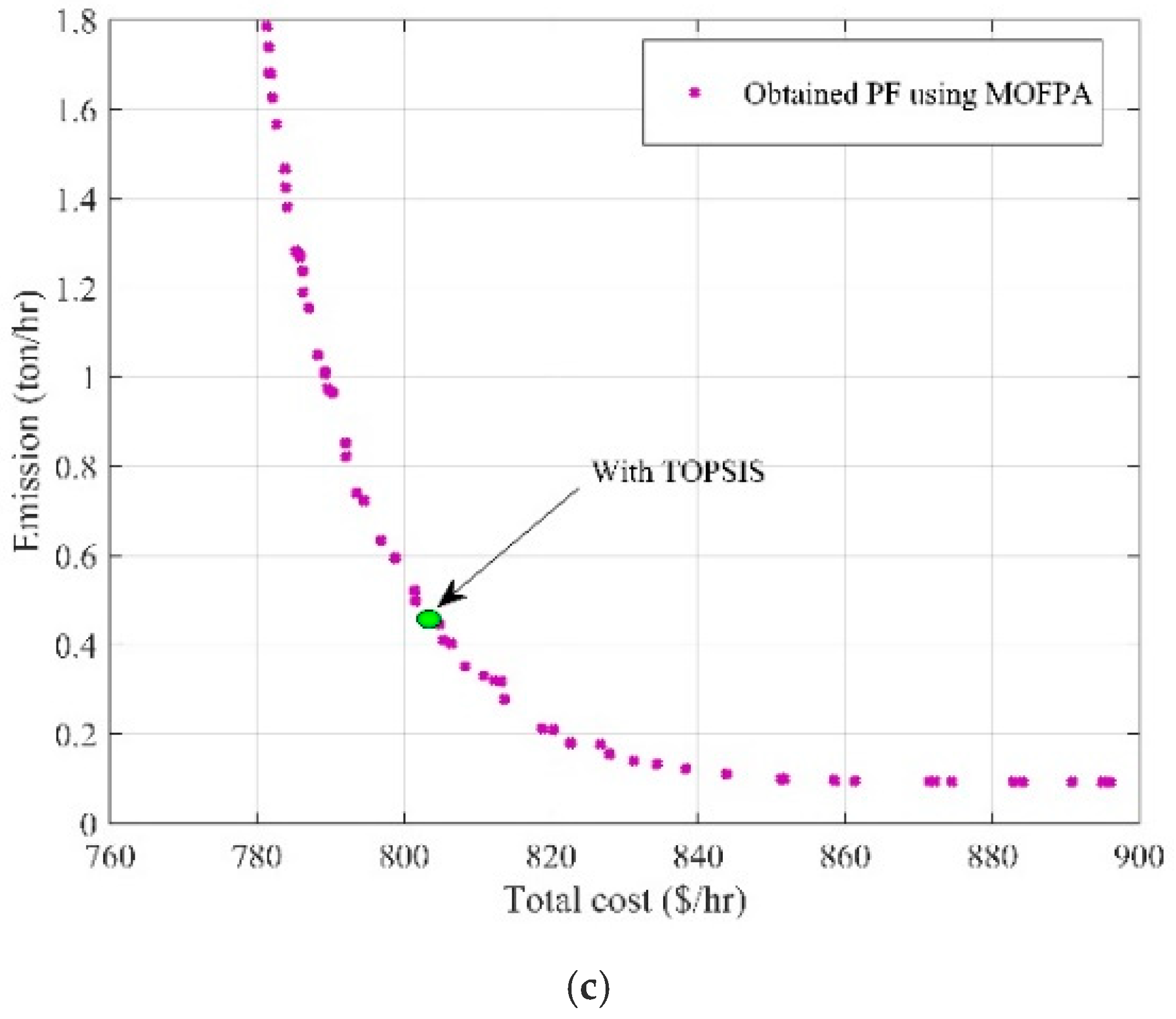
4.1. First Scenario
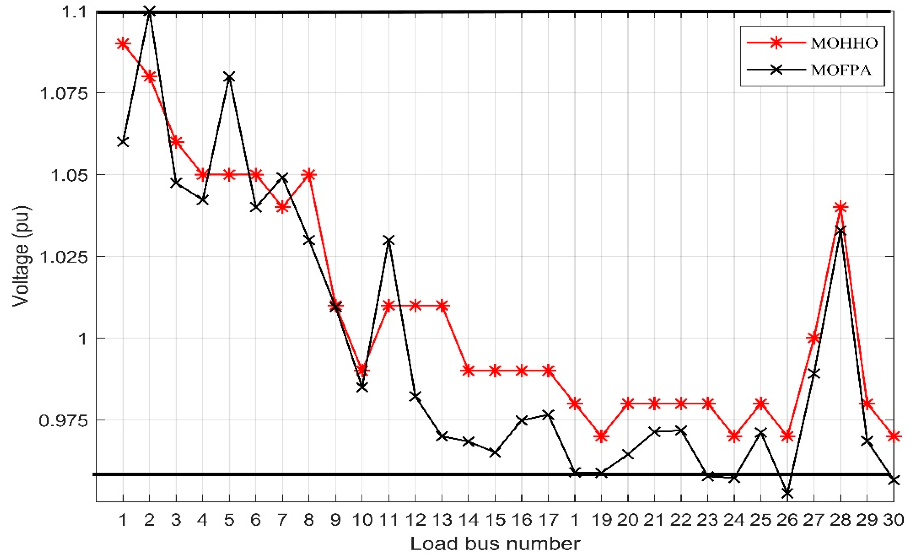
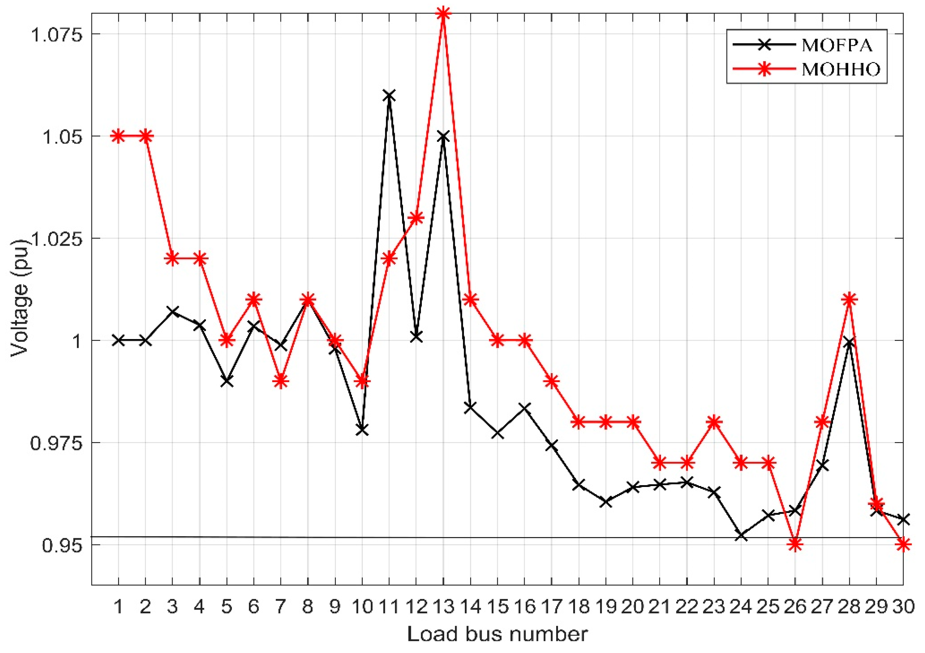
4.2. Second Scenario
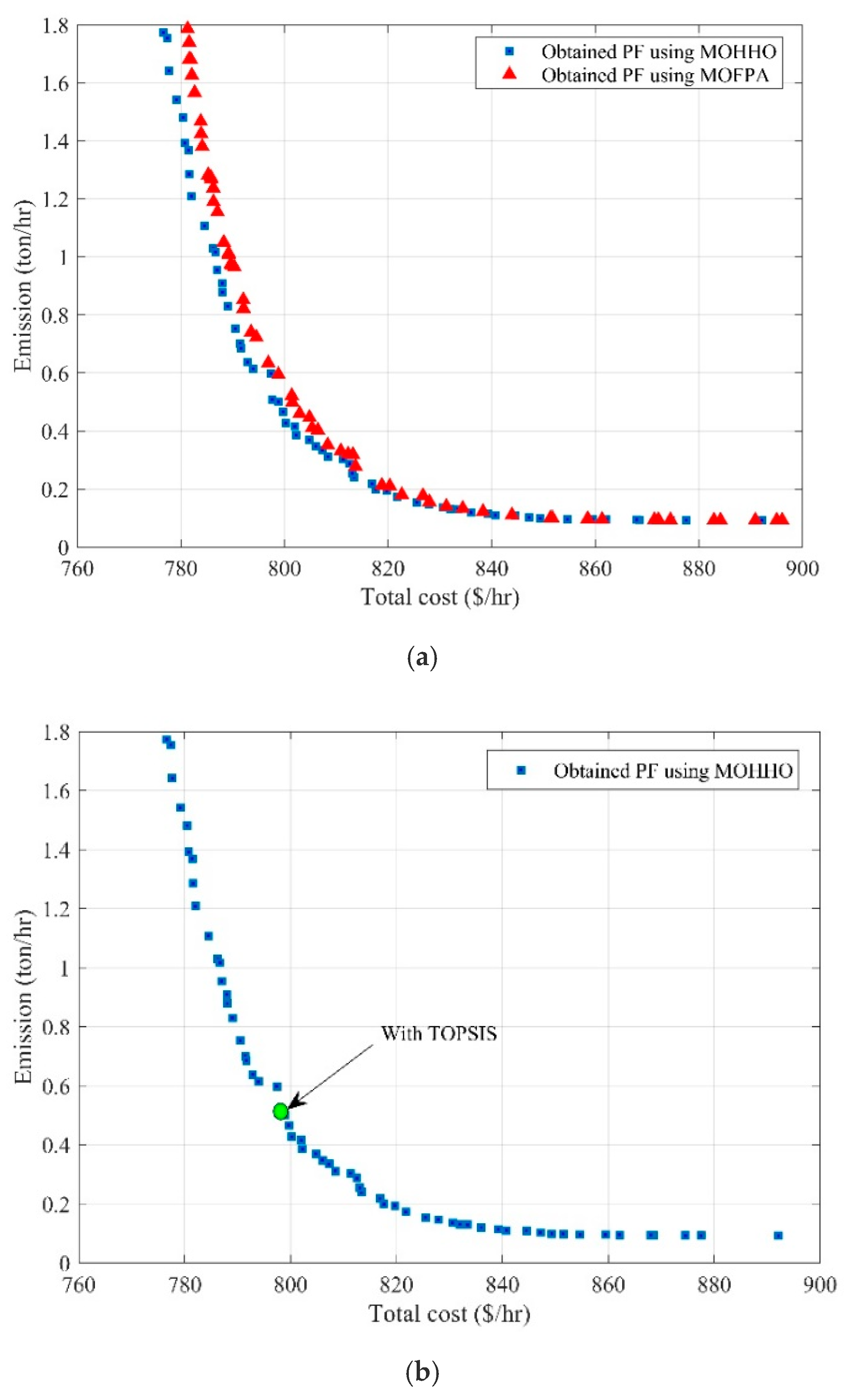
4.3. Third Scenario
5. Conclusions
Author Contributions
Funding
Conflicts of Interest
Abbreviations
| ABC | Artificial bee colony |
| ABC-DP | Dynamic population-based artificial bee colony |
| CHP | Combined heat and power |
| CS | Cuckoo search algorithm |
| DNOs | Distribution network operators |
| EED | Environmental economic dispatch |
| ES | Energy storage |
| HHV | High heat value of natural gas |
| IMFO | Improved multi-objective moth-flame optimization |
| ISA | Interior search algorithm |
| IWOA | The improved whale optimization algorithm |
| MADM | Multi-attribute decision making |
| MARL | Multi-agent reinforcement learning |
| MOCE/D | Multi-objective cross-entropy algorithm based on decomposition |
| MOEED | Multi-objective environmental economic dispatch |
| MOEA/D | Decomposition-based multi-objective evolutionary algorithm |
| MOFPA | Multi-objective flower pollination algorithm |
| MOGOA | Multi-objective grasshopper optimization algorithm |
| MOHHO | Multi-objective Harris hawks optimization |
| MOMFO | Multi-objective moth-flame optimization |
| MOO | Multi-objective optimization |
| MOPEO | Multi-objective population extremal optimization |
| MOPSO | Multi-objective particle swarm optimization |
| MOSSA | Multi-objective salp search algorithm |
| MOZSA | Multi-objective zigzag search algorithm |
| NG | Natural gas |
| NGUs | Natural gas units |
| NSGA | Non-dominated sorting genetic algorithm |
| PDFs | Probability density functions |
| PFs | Pareto fronts |
| POF | Pareto optimal front |
| POZs | Prohibited operating zones |
| RC | Relative closeness to the ideal solution |
| SF | Feasible solution |
| SMODE | Summation based multi-objective differential evolution |
| SSA | Salp swarm algorithm |
| TLBO | Teaching learning-based optimization |
| TOPSIS | The technique for order preference by similarity to an ideal solution |
| TPGUs | Thermal power generation units |
| TVAC | Time-varying acceleration coefficient |
| VD | Voltage deviation |
| VRESs | Variable renewable energy sources |
Nomenclature
| The scale factor of the wind turbine | |
| The shape factor of the wind turbine | |
| The direct cost of the photovoltaic system | |
| The direct cost of the photovoltaic-small hydro system | |
| The direct cost of the wind turbine | |
| The constant-coefficient of natural gas | |
| The reserve capacity cost of the photovoltaic system | |
| The reserve capacity cost of the photovoltaic-small hydro system | |
| The reserve capacity cost of the wind turbine | |
| The storage units cost of the photovoltaic system | |
| The storage units cost of the photovoltaic-small hydro system | |
| The storage units cost of the wind turbine | |
| The total cost of the fuel or generation | |
| The total cost of the photovoltaic generation unit | |
| The total cost of the photovoltaic-small hydro generation unit | |
| The total cost of the wind turbine generation unit | |
| The total cost of the natural gas unit | |
| The total cost of the thermal power generation unit | |
| The total cost of the variable renewable energy sources | |
| The phase difference between the buses i and j | |
| The internal diameter of the pipe in millimeters | |
| The efficiency of the gas turbine | |
| The efficiency of hydro turbine generator | |
| The total emission | |
| The probability of wind speed | |
| Friction factor | |
| γ | Scale parameter of the river |
| Initial and operation costs coefficient for ith natural gas units | |
| G | Solar irradiance |
| Standard solar irradiance | |
| The transconductance of branch q connected to bus i and bus j | |
| The effective pressure head for the water | |
| The direct cost parameter of the wind turbine | |
| The reserve capacity cost parameter of the wind turbine | |
| The storage unit cost parameter of the wind turbine | |
| λ | Location parameter of the river |
| Length of pipeline in meters | |
| Number of generator buses | |
| Number of load buses | |
| Number of branches in the network | |
| Absolute upstream (inlet) pressure | |
| Absolute downstream (outlet) pressure | |
| Absolute pressure | |
| Network power loss | |
| Pipeline pressure | |
| The actual power of the photovoltaic system | |
| The rated power of the photovoltaic system | |
| The scheduled power of the photovoltaic system | |
| The actual power of the photovoltaic small hydro system | |
| The scheduled power of the photovoltaic-small hydro system | |
| The minimum power of the ith thermal power generator unit | |
| The actual power of the wind turbine | |
| The rated power of the wind turbine | |
| The scheduled power of the wind turbine | |
| River flow rate | |
| Operation irradiance | |
| Water density | |
| The branches’ capacity limit | |
| The specific gravity of natural gas | |
| The average temperature of the flowing gas in kelvin | |
| The standard temperature in kelvin | |
| The flow velocity of the natural gas in m/sec | |
| The wind speed | |
| The voltage of the ith on generator bus | |
| Cut-in speed of the wind turbine | |
| The voltage of the pth on load bus | |
| Volume on the remind loads of the natural gas | |
| Cut-out speed of the wind turbine | |
| The rated speed of the wind turbine | |
| Average compressibility factor of natural gas |
Appendix A

| Wind (Bus 5) | Solar (Bus 11) | Solar-Hydro (Bus 13) | |
|---|---|---|---|
| Direct cost parameters ($/MW) | = 1.7 | = 1.6 | = 1.5 |
| Reserve cost parameters ($/MW) | = 3 | = 3 | = 3 |
| Penalty cost parameters ($/MW) | = 1.4 | = 1.4 | = 1.4 |
References
- Deng, X.; Lv, T. Power system planning with increasing variable renewable energy: A review of optimization models. J. Clean. Prod. 2020, 246. [Google Scholar] [CrossRef]
- Yin, L.; Gao, Q.; Zhao, L.; Wang, T. Expandable deep learning for real-time economic generation dispatch and control of three-state energies based future smart grids. Energy 2020, 191, 116561. [Google Scholar] [CrossRef]
- Lin, Z.; Chen, H.; Wu, Q.; Li, W.; Li, M.; Ji, T. Mean-tracking model based stochastic economic dispatch for power systems with high penetration of wind power. Energy 2020, 193, 116826. [Google Scholar] [CrossRef] [Green Version]
- Wu, Y.; Wang, X.; Xu, Y.; Fu, Y. Multi-objective Differential-Based Brain Storm Optimization for Environmental Economic Dispatch Problem. In Adaptation, Learning, and Optimization; Cheng, S., Shi, Y., Eds.; Springer International Publishing: Cham, Germany, 2019; Volume 23, pp. 79–104. ISBN 978-3-030-15070-9. [Google Scholar]
- El-Sayed, W.T.; El-Saadany, E.F.; Zeineldin, H.H.; Al-Sumaiti, A.S. Fast initialization methods for the nonconvex economic dispatch problem. Energy 2020, 201, 117635. [Google Scholar] [CrossRef]
- Kaboli, S.H.A.; Alqallaf, A.K. Solving non-convex economic load dispatch problem via artificial cooperative search algorithm. Expert Syst. Appl. 2019, 128, 14–27. [Google Scholar] [CrossRef]
- Ismael, S.M.; Abdel Aleem, S.H.E.; Abdelaziz, A.Y.; Zobaa, A.F. State-of-the-art of hosting capacity in modern power systems with distributed generation. Renew. Energy 2019, 130, 1002–1020. [Google Scholar] [CrossRef]
- Rizk-Allah, R.M.; Abdel Mageed, H.M.; El-Sehiemy, R.A.; Abdel Aleem, S.H.E.; El Shahat, A. A new sine cosine optimization algorithm for solving combined non-convex economic and emission power dispatch problems. Int. J. Energy Convers. 2017, 5, 180. [Google Scholar] [CrossRef]
- Zhang, X.-P.; Ou, M.; Song, Y.; Li, X. Review of Middle East energy interconnection development. J. Mod. Power Syst. Clean Energy 2017, 5, 917–935. [Google Scholar] [CrossRef] [Green Version]
- Ismael, S.M.; Abdel Aleem, S.H.E.; Abdelaziz, A.Y.; Zobaa, A.F. Practical considerations for optimal conductor reinforcement and hosting capacity enhancement in radial distribution systems. IEEE Access 2018, 6, 27268–27277. [Google Scholar] [CrossRef]
- Qu, B.Y.; Zhu, Y.S.; Jiao, Y.C.; Wu, M.Y.; Suganthan, P.N.; Liang, J.J. A survey on multi-objective evolutionary algorithms for the solution of the environmental/economic dispatch problems. Swarm Evol. Comput. 2018, 38, 1–11. [Google Scholar] [CrossRef]
- Khaled, M.; Sayah, S.; Bekrar, A. Whale optimization algorithm based optimal reactive power dispatch: A case study of the Algerian power system. Electr. Power Syst. Res. 2018, 163, 696–705. [Google Scholar] [CrossRef]
- Mason, K.; Duggan, J.; Howley, E. Multi-objective dynamic economic emission dispatch using particle swarm optimisation variants. Neurocomputing 2017, 270, 188–197. [Google Scholar] [CrossRef]
- Karthik, N.; Parvathy, A.K.; Arul, R. Multi-objective economic emission dispatch using interior search algorithm. Int. Trans. Electr. Energy Syst. 2019, 29, e2683. [Google Scholar] [CrossRef] [Green Version]
- Nourianfar, H.; Abdi, H. Solving the multi-objective economic emission dispatch problems using Fast Non-Dominated Sorting TVAC-PSO combined with EMA. Appl. Soft Comput. 2019, 85, 105770. [Google Scholar] [CrossRef]
- Elsakaan, A.A.; El-Sehiemy, R.A.; Kaddah, S.S.; Elsaid, M.I. An enhanced moth-flame optimizer for solving non-smooth economic dispatch problems with emissions. Energy 2018, 157, 1063–1078. [Google Scholar] [CrossRef]
- El Sehiemy, R.A.; Selim, F.; Bentouati, B.; Abido, M.A. A novel multi-objective hybrid particle swarm and salp optimization algorithm for technical-economical-environmental operation in power systems. Energy 2020, 193, 116817. [Google Scholar] [CrossRef]
- Ding, M.; Chen, H.; Lin, N.; Jing, S.; Liu, F.; Liang, X.; Liu, W. Dynamic population artificial bee colony algorithm for multi-objective optimal power flow. Saudi J. Biol. Sci. 2017, 24, 703–710. [Google Scholar] [CrossRef]
- Liang, R.-H.; Wu, C.-Y.; Chen, Y.-T.; Tseng, W.-T. Multi-objective dynamic optimal power flow using improved artificial bee colony algorithm based on Pareto optimization. Int. Trans. Electr. Energy Syst. 2016, 26, 692–712. [Google Scholar] [CrossRef]
- Biswas, P.P.; Suganthan, P.N.; Mallipeddi, R.; Amaratunga, G.A.J. Multi-objective optimal power flow solutions using a constraint handling technique of evolutionary algorithms. Soft Comput. 2020, 24, 2999–3023. [Google Scholar] [CrossRef]
- Wang, G.; Zha, Y.; Wu, T.; Qiu, J.; Peng, J.; Xu, G. Cross entropy optimization based on decomposition for multi-objective economic emission dispatch considering renewable energy generation uncertainties. Energy 2020, 193, 116790. [Google Scholar] [CrossRef]
- Chen, M.-R.; Zeng, G.-Q.; Lu, K.-D. Constrained multi-objective population extremal optimization based economic-emission dispatch incorporating renewable energy resources. Renew. Energy 2019, 143, 277–294. [Google Scholar] [CrossRef]
- Bora, T.C.; Mariani, V.C.; dos Santos Coelho, L. Multi-objective optimization of the environmental-economic dispatch with reinforcement learning based on non-dominated sorting genetic algorithm. Appl. Therm. Eng. 2019, 146, 688–700. [Google Scholar] [CrossRef]
- Biswas, P.P.; Suganthan, P.N.; Qu, B.Y.; Amaratunga, G.A.J. Multiobjective economic-environmental power dispatch with stochastic wind-solar-small hydro power. Energy 2018, 150, 1039–1057. [Google Scholar] [CrossRef]
- Yin, Y.; Liu, T.; He, C. Day-ahead stochastic coordinated scheduling for thermal-hydro-wind-photovoltaic systems. Energy 2019, 187, 115944. [Google Scholar] [CrossRef]
- Li, X.; Wang, W.; Wang, H.; Wu, J.; Fan, X.; Xu, Q. Dynamic environmental economic dispatch of hybrid renewable energy systems based on tradable green certificates. Energy 2020, 193, 116699. [Google Scholar] [CrossRef]
- Elattar, E.E. Environmental economic dispatch with heat optimization in the presence of renewable energy based on modified shuffle frog leaping algorithm. Energy 2019, 171, 256–269. [Google Scholar] [CrossRef]
- Joshi, P.M.; Verma, H.K. An improved TLBO based economic dispatch of power generation through distributed energy resources considering environmental constraints. Sustain. Energy Grids Netw. 2019, 18, 100207. [Google Scholar] [CrossRef]
- Bai, W.; Eke, I.; Lee, K.Y. An improved artificial bee colony optimization algorithm based on orthogonal learning for optimal power flow problem. Control Eng. Pract. 2017, 61, 163–172. [Google Scholar] [CrossRef]
- Biswas, P.P.; Suganthan, P.N.; Amaratunga, G.A.J. Optimal power flow solutions incorporating stochastic wind and solar power. Energy Convers. Manag. 2017, 148, 1194–1207. [Google Scholar] [CrossRef]
- Hulio, Z.H.; Jiang, W.; Rehman, S. Techno—Economic assessment of wind power potential of Hawke’s Bay using Weibull parameter: A review. Energy Strateg. Rev. 2019, 26, 100375. [Google Scholar] [CrossRef]
- Panda, A.; Tripathy, M. Security constrained optimal power flow solution of wind-thermal generation system using modified bacteria foraging algorithm. Energy 2015, 93, 816–827. [Google Scholar] [CrossRef]
- Zhai, R.; Liu, H.; Chen, Y.; Wu, H.; Yang, Y. The daily and annual technical-economic analysis of the thermal storage PV-CSP system in two dispatch strategies. Energy Convers. Manag. 2017, 154, 56–67. [Google Scholar] [CrossRef]
- Tan, Q.; Mei, S.; Dai, M.; Zhou, L.; Wei, Y.; Ju, L. A multi-objective optimization dispatching and adaptability analysis model for wind-PV-thermal-coordinated operations considering comprehensive forecasting error distribution. J. Clean. Prod. 2020, 256, 120407. [Google Scholar] [CrossRef]
- Gómez, Y.M.; Bolfarine, H.; Gómez, H.W. Gumbel distribution with heavy tails and applications to environmental data. Math. Comput. Simul. 2019, 157, 115–129. [Google Scholar] [CrossRef]
- Tso, W.W.; Demirhan, C.D.; Floudas, C.A.; Pistikopoulos, E.N. Multi-scale energy systems engineering for optimal natural gas utilization. Catal. Today 2019. [Google Scholar] [CrossRef]
- Chen, S.; Wei, Z.; Sun, G.; Wang, D.; Zhang, Y.; Ma, Z. Stochastic look-ahead dispatch for coupled electricity and natural-gas networks. Electr. Power Syst. Res. 2018, 164, 159–166. [Google Scholar] [CrossRef]
- Algabalawy, M.A.; Abdelaziz, A.Y.; Mekhamer, S.F.; Abdel Aleem, S.H.E. Considerations on optimal design of hybrid power generation systems using whale and sine cosine optimization algorithms. J. Electr. Syst. Inf. Technol. 2018, 5, 312–325. [Google Scholar] [CrossRef]
- Li, G.; Zhang, R.; Jiang, T.; Chen, H.; Bai, L.; Li, X. Security-constrained bi-level economic dispatch model for integrated natural gas and electricity systems considering wind power and power-to-gas process. Appl. Energy 2017, 194, 696–704. [Google Scholar] [CrossRef]
- Avalos, R.; Fitzgerald, T.; Rucker, R.R. Measuring the effects of natural gas pipeline constraints on regional pricing and market integration. Energy Econ. 2016, 60, 217–231. [Google Scholar] [CrossRef] [Green Version]
- Abul’Wafa, A.R. Optimization of economic/emission load dispatch for hybrid generating systems using controlled Elitist NSGA-II. Electr. Power Syst. Res. 2013, 105, 142–151. [Google Scholar] [CrossRef]
- Dhanalakshmi, S.; Kannan, S.; Mahadevan, K.; Baskar, S. Application of modified NSGA-II algorithm to Combined Economic and Emission Dispatch problem. Int. J. Electr. Power Energy Syst. 2011, 33, 992–1002. [Google Scholar] [CrossRef]
- Zhao, F.; Yuan, J.; Wang, N. Dynamic economic dispatch model of microgrid containing energy storage components based on a variant of NSGA-II Algorithm. Energies 2019, 12, 871. [Google Scholar] [CrossRef] [Green Version]
- Basu, M. Combined heat and power economic emission dispatch using nondominated sorting genetic algorithm-II. Int. J. Electr. Power Energy Syst. 2013, 53, 135–141. [Google Scholar] [CrossRef]
- Yang, X.-S.; Karamanoglu, M.; He, X. Flower pollination algorithm: A novel approach for multiobjective optimization. Eng. Optim. 2014, 46, 1222–1237. [Google Scholar] [CrossRef] [Green Version]
- Abdelaziz, A.Y.; Ali, E.S.; Abd Elazim, S.M. Flower pollination algorithm to solve combined economic and emission dispatch problems. Eng. Sci. Technol. Int. J. 2016, 19, 980–990. [Google Scholar] [CrossRef] [Green Version]
- Heidari, A.A.; Mirjalili, S.; Faris, H.; Aljarah, I.; Mafarja, M.; Chen, H. Harris hawks optimization: Algorithm and applications. Future Gener. Comput. Syst. 2019, 97, 849–872. [Google Scholar] [CrossRef]
- Aleem, S.H.E.A.; Zobaa, A.F.; Balci, M.E.; Ismael, S.M. Harmonic overloading minimization of frequency-dependent components in harmonics polluted distribution systems using harris hawks optimization algorithm. IEEE Access 2019, 7, 100824–100837. [Google Scholar] [CrossRef]
- Lin, Y.-K.; Chang, P.-C.; Yeng, L.C.-L.; Huang, S.-F. Bi-objective optimization for a multistate job-shop production network using NSGA-II and TOPSIS. J. Manuf. Syst. 2019, 52, 43–54. [Google Scholar] [CrossRef]
- Deb, M.; Debbarma, B.; Majumder, A.; Banerjee, R. Performance-emission optimization of a diesel-hydrogen dual fuel operation: A NSGA II coupled TOPSIS MADM approach. Energy 2016, 117, 281–290. [Google Scholar] [CrossRef]
- Zhang, H.; Lu, Z.; Hu, W.; Wang, Y.; Dong, L.; Zhang, J. Coordinated optimal operation of hydro-wind-solar integrated systems. Appl. Energy 2019, 242, 883–896. [Google Scholar] [CrossRef]


| Ref. | Year | Systems Used | Optimization Techniques | Comparative Analysis | Objective Functions * | Ranking Method | Comments | |||
|---|---|---|---|---|---|---|---|---|---|---|
| 1 | 2 | 3 | 4 | |||||||
| [12] | 2018 | IEEE 14-bus, IEEE 30-bus and Algerian 114-bus | IWOA | PSO PSO-TVAC | ✗ | ✗ | ✓ | ✗ | ✗ | Different cases are examined. No ranking method is used to get the best solution |
| [13] | 2017 | Hypothetical system | PSO | NSGA-II MARL | ✓ | ✓ | ✗ | ✗ | ✗ | The aims are to test different variants of PSO. Many constraints are not considered. |
| [14] | 2019 | 3, 10, 20 and 40 generating units and IEEE 30-bus | ISA | GA FPA CS ABC | ✓ | ✓ | ✗ | ✗ | ✗ | POZ and valve point effects constraints are not considered. |
| [15] | 2019 | 48-unit CHP | TVAC-PSO | FCM | ✓ | ✓ | ✗ | ✗ | ✓ | Spinning reserve requirements, ramp rate limits, valve points effects, and multiple fuel units are considered as additional constraints. TOPSIS is utilized to get the best optimal solutions. |
| [16] | 2018 | 6, 40 and 80 generating units | IMFO | FPA GA PSO | ✓ | ✓ | ✗ | ✗ | ✗ | Multi-objective optimization is transformed into a single objective, which made the problem simple. No ranking method is utilized. Some constraints are not considered. |
| [17] | 2017 | IEEE 30-bus | ABC-DP | NSGA-II MOABC | ✓ | ✓ | ✓ | ✗ | ✗ | Only equality and inequality constraints are considered. |
| [18] | 2016 | IEEE 30-bus IEEE 118-bus | ABC | IABC GA DE | ✓ | ✓ | ✓ | ✗ | ✗ | Operators can select one of the non-dominated solutions according to the situation. Some constraints are not considered. |
| [19] | 2020 | IEEE 30-bus IEEE 57-bus IEEE 118-bus | SSA-PSO | ABC GA DE WOA | ✓ | ✓ | ✓ | ✓ | ✗ | Transformer tapping limits, voltage magnitude limits of load buses, and power flow limits of transmission lines are considered as inequality constraints. No ranking method is employed to get the best solution. |
| [20] | 2019 | IEEE 30-bus IEEE 57-bus | MOEA/D | MTLBO MGBICA MOICA | ✓ | ✓ | ✓ | ✓ | ✗ | POZ and valve point effects constraints are not considered. No ranking method is employed to obtain the best solution. |
| Ref. | Year | Test System | Optimization Techniques | Comparative Analysis | Objective Functions * | Ranking Index | Comments | |||
|---|---|---|---|---|---|---|---|---|---|---|
| 1 | 2 | 3 | 4 | |||||||
| [21] | 2020 | IEEE 30 IEEE 118 | MOCE/D | PSO NSGA-II | ✓ | ✓ | ✗ | ✗ | ✗ | Valve point effects are not considered. No ranking method is employed to get the best solution. |
| [22] | 2019 | IEEE 30 | MOPEO | DE NSGA-II | ✓ | ✓ | ✗ | ✗ | ✗ | Other sources such as small-hydro power and electric vehicles are not considered in the problem formulation. |
| [23] | 2019 | IEEE 30 | NSGA-RL | NSGA-II | ✓ | ✓ | ✗ | ✗ | ✓ | Generational distance and spread of evaluation performance matrices are used to get the best optimal solution. |
| [24] | 2018 | IEEE 30 | MOEA/D SMODE | ✗ | ✓ | ✓ | ✗ | ✗ | ✗ | Stochastic natures of VRESs are considered. The obtained results were not compared to other algorithms to evaluate its performance. |
| [25] | 2019 | 6 bus power system | Copula function | ✗ | ✓ | ✗ | ✗ | ✗ | ✗ | Single objective optimization is applied. No ranking method is used. Some constraints are not considered. |
| [26] | 2020 | IEEE 39 | MOMFO | NSGA-II MOPSO | ✗ | ✓ | ✗ | ✗ | ✗ | Multi-objective functions are not considered. Only equality and inequality constraints are considered. |
| [27] | 2019 | Different test systems | MSFLA | SLFA GA TLBO | ✓ | ✓ | ✗ | ✗ | ✗ | Single objective optimization is applied. Various constraints are included. Valve point effects are not considered. |
| [28] | 2019 | Different systems | TLBO-PSO | GA CTLBO | ✓ | ✓ | ✗ | ✗ | ✗ | Multi-objective functions are investigated. Various constraints are not considered such as valve point effects. |
| Item | Quantity | Specifications |
|---|---|---|
| Generators | 6 | 3 TPGUs and 3 VRESs |
| TPGUs | 3 | Bus 1 (slack), bus 2, and bus 8 |
| Wind turbine (WT) | 25 | Bus 5, 75 MW |
| Photovoltaic array (PV) | 1 | Bus 11, 50 MW |
| Hybrid PV and small-hydro (PVSH) | 1 | Bus 13, 45 + 5 MW |
| Active load demand | - | 283.4 MW |
| Reactive load demand | - | 126.2 MVAr |
| Number of PQ buses | 24 | 24 load buses |
| Minimum load voltage allowed | - | 0.95 pu |
| Maximum load voltage allowed | - | 1.10 pu |
| Emission Parameters | ||||||
| Generator | Bus | |||||
| (t/h) | (t/pu. MWh) | (t/pu. MW2h) | (t/h) | (pu. MW−1) | ||
| TPGU1 | 1 | 0.04091 | −0.05554 | 0.0649 | 0.0002 | 6.667 |
| TPGU2 | 2 | 0.02543 | −0.06047 | 0.05638 | 0.0005 | 3.333 |
| TPGU3 | 8 | 0.05326 | −0.0355 | 0.0338 | 0.002 | 2 |
| Cost Parameters | ||||||
| Generator | Bus | |||||
| ($/h) | ($/MWh) | ($/MW2h) | ($/h) | (MW−1) | ||
| TPGU1 | 1 | 30 | 2 | 0.00375 | 18 | 0.037 |
| TPGU2 | 2 | 25 | 1.75 | 0.0175 | 16 | 0.038 |
| TPGU3 | 8 | 20 | 3.25 | 0.00834 | 12 | 0.045 |
| Emission Parameters | ||||
| Generator | Bus | |||
| (t/h) | (t/pu. MWh) | (t/pu. MW2h) | ||
| NGU1 | 1 | 0.02091 | −0.07554 | 0.04490 |
| NGU2 | 2 | 0.02543 | −0.05047 | 0.03638 |
| NGU3 | 8 | 0.03326 | −0.05550 | 0.01380 |
| Cost Parameters | ||||
| Generator | Bus | |||
| ($/h) | ($/MWh) | ($/MW2h) | ||
| NGU1 | 1 | 14 | 1.06 | 0.00175 |
| NGU2 | 2 | 15 | 1.05 | 0.0105 |
| NGU3 | 8 | 17 | 1.25 | 0.02434 |
| State Variables | Min. | Max. | MOEA/D | SMODE |
|---|---|---|---|---|
| PNGU1 (MW) | 50 | 140 | 117.118 | 111.91 |
| PTPGU2 (MW) | 20 | 80 | 65 | 65 |
| PTPGU3 (MW) | 10 | 35 | 18.403 | 23.555 |
| Pw (MW) | 0 | 75 | 55.447 | 54.058 |
| Ppv (MW) | 0 | 50 | 17.649 | 18.436 |
| Ppvh (MW) | 0 | 50 | 15.326 | 15.755 |
| Q1 (MVAr) | −50 | 140 | 2.128 | 2.788 |
| Q2 (MVAr) | −20 | 60 | 21.41 | 34.504 |
| Q5 (MVAr) | −15 | 70 | 37.727 | 36.169 |
| Q8 (MVAr) | −30 | 60 | 27.102 | 20.376 |
| Q11 (MVAr) | −20 | 30 | 24.911 | 23.41 |
| Q13 (MVAr) | −20 | 25 | 20.328 | 15.62 |
| V1 (pu) | 0.96 | 1.10 | 1.076 | 1.0761 |
| V2 (pu) | 0.96 | 1.10 | 1.0648 | 1.0662 |
| V5 (pu) | 0.96 | 1.10 | 1.0444 | 1.0362 |
| V8 (pu) | 0.96 | 1.10 | 1.0402 | 1.0362 |
| V11 (pu) | 0.96 | 1.10 | 1.0878 | 1.0778 |
| V13 (pu) | 0.96 | 1.10 | 1.0602 | 1.0432 |
| Ploss (MW) | 5.5429 | 5.3148 | ||
| VD (pu) | 0.4530 | 0.4215 | ||
| Total cost ($/h) | 919.040 | 927.049 | ||
| Emission (t/h) | 0.6221 | 0.4721 |
| State Variables | Min. | Max. | MOHHO | MOFPA |
|---|---|---|---|---|
| PTPGU1 (MW) | 50 | 140 | 72.84 | 64.86 |
| PTPGU2 (MW) | 20 | 80 | 80.00 | 74.20 |
| PTPGU3 (MW) | 10 | 35 | 35.00 | 34.97 |
| Pw (MW) | 0 | 75 | 33.74 | 31.35 |
| Ppv (MW) | 0 | 50 | 39.73 | 39.60 |
| Ppvh (MW) | 0 | 50 | 28.43 | 37.83 |
| Q1 (MVAr) | −50 | 140 | 27.31 | −29.19 |
| Q2 (MVAr) | −20 | 60 | 16.33 | 67.74 |
| Q5 (MVAr) | −15 | 70 | 30.88 | 64.07 |
| Q8 (MVAr) | −30 | 60 | 51.18 | 28.01 |
| Q11 (MVAr) | −20 | 30 | 2.45 | 11.82 |
| Q13 (MVAr) | −20 | 25 | 3.45 | −8.32 |
| V1 (pu) | 0.96 | 1.10 | 1.09 | 1.06 |
| V2 (pu) | 0.96 | 1.10 | 1.08 | 1.10 |
| V5 (pu) | 0.96 | 1.10 | 1.05 | 1.08 |
| V8 (pu) | 0.96 | 1.10 | 1.05 | 1.03 |
| V11 (pu) | 0.96 | 1.10 | 1.01 | 1.03 |
| V13 (pu) | 0.96 | 1.10 | 1.01 | 0.97 |
| Ploss (MW) | 4.50 | 4.89 | ||
| VD (pu) | 0.56 | 0.79 | ||
| Wgencost | 102.39 | 124.88 | ||
| Sgencost | 147.24 | 150.24 | ||
| Shgencost | 97.38 | 143.72 | ||
| mass flow (m3) | 63.55 | 71.36401 | ||
| Emission of P2 and P3 (t/h) | 0.0691 | 0.066868 | ||
| Emission of P1 (t/h) | 0.0154 | 0.005905 | ||
| P1_cost | 9.53 | 10.7046 | ||
| Total cost ($/h) | 798.18 | 804.58 | ||
| Emission (t/h) | 0.5221 | 0.4521 | ||
| Fuelvlvcost | 340.82 | 327.40 |
| State Variables | Min | Max | MOHHO | MOFPA |
|---|---|---|---|---|
| PTPGU1 (MW) | 50 | 140 | 121.48 | 52.81 |
| PNGU2 (MW) | 20 | 80 | 80.00 | 80.00 |
| PTPGU3 (MW) | 10 | 35 | 35.00 | 43.19 |
| Pw (MW) | 0 | 75 | 69.56 | 52.29 |
| Ppv (MW) | 0 | 50 | 23.93 | 32.95 |
| Ppvh (MW) | 0 | 50 | 18.55 | 28.58 |
| Q1 (MVAr) | −50 | 140 | 30.12 | −5.72 |
| Q2 (MVAr) | −20 | 60 | −5.86 | 6.15 |
| Q5 (MVAr) | −15 | 40 | 17.85 | 36.58 |
| Q8 (MVAr) | −30 | 35 | 48.55 | 49.17 |
| Q11 (MVAr) | −20 | 25 | 5.52 | 17.46 |
| Q13 (MVAr) | −20 | 25 | 45.68 | 26.71 |
| V1 (pu) | 0.96 | 1.10 | 1.05 | 1.00 |
| V2 (pu) | 0.96 | 1.10 | 1.05 | 1.00 |
| V5 (pu) | 0.96 | 1.10 | 1.00 | 0.99 |
| V8 (pu) | 0.96 | 1.10 | 1.01 | 1.01 |
| V11 (pu) | 0.96 | 1.10 | 1.02 | 1.06 |
| V13 (pu) | 0.96 | 1.10 | 1.08 | 1.05 |
| Ploss (MW) | 7.21 | 4.04 | ||
| VD (pu) | 0.50 | 0.64 | ||
| Wgencost | 99.53 | 193.20 | ||
| Sgencost | 32.90 | 51.60 | ||
| Shgencost | 27.89 | 39.78 | ||
| mass flow_02 | 172.83 | 172.83 | ||
| mass flow_08 | 75.62 | 93.31 | ||
| Total cost ($/h) | 796.35 | 807.89 | ||
| Emission (t/h) | 0.558 | 0.421 | ||
| Fuelvlvcost | 336.87 | 147.93 |
| Scenarios | Scenario I | Scenario II | Scenario III | |||
|---|---|---|---|---|---|---|
| Algorithms | MOEA/D | SMODE | MOHHO | MOFPA | MOHHO | MOFPA |
| No. of iterations | 200 | 200 | 200 | 200 | 200 | 200 |
| No. of population | 200 | 200 | 200 | 200 | 200 | 200 |
| Control parameters | = 0.9 Mutation factor = 0.5 Crossover rate = 0.9 | Mutation factor = 0.5 Crossover rate = 0.9 | = [0,1] = [0,1] | = 0.5 = 1.5 = [0,1] | = [0,1] = [0,1] | = 0.5 = 1.5 = [0,1] |
| Computation time (min) | 45.14 | 45.64 | 4.23 | 14.08 | 4.16 | 13.34 |
| Total cost ($/h) | 919.040 | 927.049 | 798.18 | 804.58 | 796.35 | 807.89 |
| Emission (t/h) | 0.6221 | 0.4721 | 0.5221 | 0.4521 | 0.558 | 0.421 |
© 2020 by the authors. Licensee MDPI, Basel, Switzerland. This article is an open access article distributed under the terms and conditions of the Creative Commons Attribution (CC BY) license (http://creativecommons.org/licenses/by/4.0/).
Share and Cite
Omar, A.I.; Ali, Z.M.; Al-Gabalawy, M.; Abdel Aleem, S.H.E.; Al-Dhaifallah, M. Multi-Objective Environmental Economic Dispatch of an Electricity System Considering Integrated Natural Gas Units and Variable Renewable Energy Sources. Mathematics 2020, 8, 1100. https://doi.org/10.3390/math8071100
Omar AI, Ali ZM, Al-Gabalawy M, Abdel Aleem SHE, Al-Dhaifallah M. Multi-Objective Environmental Economic Dispatch of an Electricity System Considering Integrated Natural Gas Units and Variable Renewable Energy Sources. Mathematics. 2020; 8(7):1100. https://doi.org/10.3390/math8071100
Chicago/Turabian StyleOmar, Ahmed I., Ziad M. Ali, Mostafa Al-Gabalawy, Shady H. E. Abdel Aleem, and Mujahed Al-Dhaifallah. 2020. "Multi-Objective Environmental Economic Dispatch of an Electricity System Considering Integrated Natural Gas Units and Variable Renewable Energy Sources" Mathematics 8, no. 7: 1100. https://doi.org/10.3390/math8071100