On Numerical Analysis of Carreau–Yasuda Nanofluid Flow over a Non-Linearly Stretching Sheet under Viscous Dissipation and Chemical Reaction Effects

Abstract

This work reports the Carreau–Yasuda nanofluid flow over a non-linearly stretching sheet viscous dissipation and chemical reaction effects. The coupled system of non-linear partial differential equations are changed into a system of linear differential equations employing similarity equations. The spectral quasi-linearization method was used to solve the linear differential equations numerically. Error norms were used to authenticate the accuracy and convergence of the numerical method. The effects of some thermophysical parameters of interest in this current study on the non-dimensional fluid velocity, concentration and temperature, the skin friction, local Nusselt and Sherwood numbers are presented graphically. Tables were used to depict the effects of selected parameters on the skin friction and the Nusselt number.

1. Introduction

Researchers have recently shown a lot of interest towards the study of non-Newtonian fluids due to their widespread applications in areas such as mining industries, where the handling of slurries and mud is done, in biology and medicine. Unlike Newtonian fluids, non-Newtonian fluids do exist abundantly in nature. Some typical examples of non-Newtonian fluids that occur commonly include chyme, blood, oil, paints and lubricants. Non-Newtonian fluids cannot be modelled using the classical Navier–Stokes equations due to the non-linear relationship between the shear stress and rate of strain at a given temperature. It is also worth mentioning that non-Newtonian fluids are more complicated to handle than Newtonian fluids, Kahshan et al. [1].

Detailed explanation and classification of non-Newtonian fluids can be found in Cioranescu et al. [2]. After viewing the demand of the required progression and viewing the nature, researchers have proposed several non-Newtonian fluid models. Shear-thinning is one of the main behavior that is exhibited by most non-Newtonian fluids. To that end, the influence of shear-thinning behavior is worth to be investigated. This class of fluids have many applications in polymer processing and multiple emulsions. In an endeavor to anticipate the rheological features of thinning fluids several models such as Ellis model, Kheyfets and Kieweg [3], cross model, Sochi [4], Carreau model, Hina et al. [5] and Carreau–Yasuda model, Mekheimes and Abd Elmabound [6], have been proposed.

Carreau–Yasuda model is among the models which have an advantage over the power-law fluid models. It is now regarded as the generalized form of the power-law model because it has two parameters $(k,n),$ whereas the Carreau–Yasuda is a five-parameter model $({\mu }_0,{\mu }_{\infty },n,a,\lambda )$, Mahmood et al. [7]. The Carreau-Yasunda model occur in many real life and industrial applications. Since it is a shearing–thinning model, the Carreau-Yasunda model can be used in physiology to replicate blood, with blood being non-Newtonian fluid. The thinning and/or thickening property can be approximated using this model with great accuracy. Andrade et al. [8] pioneered the study of the Carreau–Yasuda model to compute the drag equation for turbulent flow in a pipe. In their study, they disclosed that these five constants $({\mu }_0,{\mu }_{\infty },n,a,\lambda )$ control the turbulence in the flow within the boundary layer. They also depicted that the Carreau–Yasuda model describes the viscocity $\left({\mu }_{\infty }\right)$ at infinite shear stress and viscosity $\left({\mu }_0\right)$ at zero shear stress. Hayat et al. [9] did a numerical study on the peristalsis of a Carreau-Yasunda nanofluid by mainly focusing on the effects of Hall and Ohmic heating. Hayat et al. [10] developed and simulated a non-linear mathematical model for a Carreau–Yasuda fluid in a curved channel with slip effects. Abbasi et al. [11] analyzed the impact of applied magnetic field on the peristaltic field of the Carreau–Yasuda fluid in a curved conduct.

Shamekhi and Sadeghy [12] in their study of a lid-driven cavity flow of a Carreau–Yasuda model showed strong effect of shear-thinning behavior on its flow kinematics. Lashgari et al. [13] showed how shear-thinning/shear-thickening destabilizes/stabilizes the flow significantly when the problem is scaled with the reference zero-shear-rate viscosity when considering the Carreau–Yasuda fluids passing over a circular cylinder. Zhao et al. [14] combined the Carreau–Yasuda model and Zheng’s model to study mixed convection heat transfer of non-Newtonian fluids in a square cavity. Khan et al. [15] examined MHD flow of Carreau–Yasuda nanofluid over a non-linearly stretching sheet considering slip conditions with Joule heating and chemical reaction. Salahuddin et al. [16] numerically explored heat assignment mechanisms in squeezed flow over a sensor surface of an electrically conducting Carreau–Yasuda fluid. Hayat et al. [17] studied the mixed convective peristaltic transport of Carreau–Yasuda through an inclined channel. Migtaa and Al-Khafajy [18] examined the influence of heat transfer on the MHD oscillatory flow by Carreau–Yasuda through porous medium for shearing–thinning case in cavity and cylindrical configuration.

Thermal conductivity of nanofluids has been widely investigated by many researchers in the past three decades since the pioneering work by Choi and Eastman [19]. Nanofluids have been used in the fields where heat transfer enhancement is required as is the case in many industrial applications. It is noted that some fluids like ethylene glycol mixture, water and oil are poor heat transfer fluids, Nandkeolyar et al. [20]. Anuar and Bachok [21] investigated the classical problems of boundary layer flow and heat transfer characteristics past a semi-infinite static flat plate and past a moving semi-based nanofluid. Prakash and Suriyakumar [22] presented the influence of heat generation from two vertical plates on the hydromagnatic convective flow of nanofluid. Sharma et al. [23] analyzed the effect of Hall current on the convection in radiative magneto nanofluid. Astuti et al. [24] studied the natural convection of the nanofluids from a vertical accelerated plate in the presence of the radiation flux and magnetic field.

Hady et al. [25] investigated the effects of thermal radiation and heat transfers on a viscous nanofluid flowing over a sheet that is non-linearly stretching. Shateyi and Prakash [26] numerically analyzed heat transfer and thermal radiation effects on MHD laminar boundary layer flow over a moving surface. Krishnamurthy et al. [27] theoretically investigated the thermal radiation and chemical reaction effects on boundary layer slip flow and melting heat transfer of nanofluid induced by a non-linear stretching sheet. Elbashbeshy and Emam [28] studied the effects of thermal radiation and heat transfer over an unsteady stretching surface embedded in a porous medium.

Viscous dissipation or Joule heating refers to the generation of heat in a conductor due to the passage of an electric current. The process has quite several applications in industry and engineering. A typical example where Joule heating has found relevance is in electrical gadgets such as in light bulbs, electric stoves, electric heaters and electric fuses. Khan et al. [29] studied Joule heating in an MHD Carreau nanofluid flowing through an inclined stretching cylinder that is convective heated. Cheng and Wu [30] numerically studied viscous dissipation effects on the onset of instability for longitudinal vertices in the thermal entrance region of a horizontal parallel plate channel. Boubaker et al. [31] studied viscous dissipation effects on the thermal boundary layer of Pseudoplastic power-law non-Newtonian fluids using discretization method and the Boubaker polynomials expansion of schemes. Recently, Lund et al. [32] analyzed the effects of viscous dissipation in heat transfer of MHD flow of micropolar fluid partial slip conditions.

The main objective of this current study is to investigate the magnetohydrodynamic flow of the Carreau–Yasuda nanofluid over a non-linear stretching sheet subjected to slip, convective and zero normal flux conditions with viscous dissipation, thermal radiation and chemical reaction. As best known by the authors of this work, there is no study that has been reported on this kind of physical phenomenon for the Carreau–Yasuda model. Motivated by the above mentioned studies, the current study seeks to fill the existing gaps in this field of research. Using well-chosen similarity transformations, the system of the defining partial differential equations is transformed into a system of ordinary differential equations. The transformed differential equations and the associated boundary conditions are solved numerically using the spectral quasi-linearization method (SQLM) which was introduced by Motsa et al. [33]. The SQLM has been successfully used by researchers to solve coupled systems of non-linear differential problems. Alharbey et al. [34] used the SQLM to investigate micropolar fluid over a horizontal plate embedded in a non-Darcy porous medium. Pal et al. [35] successfully used the SQLM to analyze entropy generation of a steady laminar two-dimensional convective magnetohydrodynamic Jeffrey nanofluid flow over a linear stretching sheet. The spectral quasi-linearization method was used by Das et al. [36] to study the Casson fluid with homogeneous heterogeneous reaction with non-linear thermal radiation over an exponential stretching sheet. In all these studies, the SQLM was found to be accurate, computationally efficient and reliable. It is due to these attributes of the numerical method that encouraged the authors of this work to consider using the SQLM.

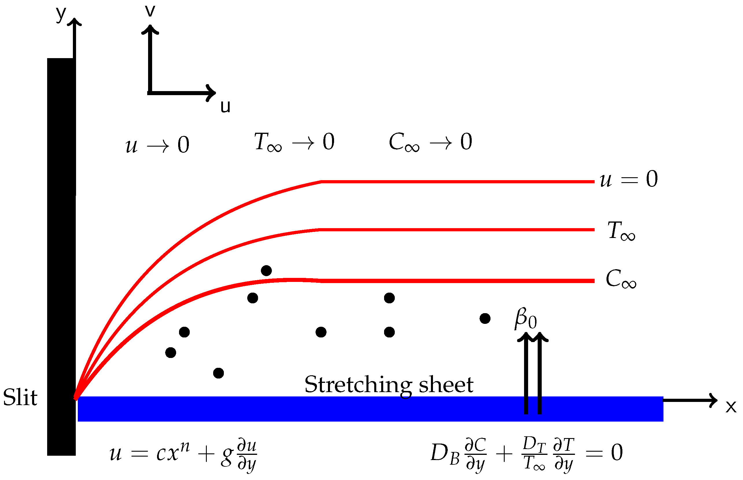
2. Mathematical Formulation

Considered in this present analysis, is a two-dimensional, steady MHD laminar incompressible flow of a Carreau–Yasuda nanofluid flow over a stretching sheet under slip and convective boundary conditions. As shown in Figure 1, the flow is taken on $y>0$, y is vertical to the stretching plate and x is along the plate. A transverse magnetic field is applied to the surface along the y axis. The non-Newtonian viscosity of a Carreau–Yasuda fluid is defined by Khan et al. [15].

$$\tau =\left[{\mu }_{\infty }+({\mu }_0-{\mu }_{\infty })(1+{\left(\Gamma \dot{\gamma }{)}^d\right)}^{\frac{n-1}{d}}\right]A_1,$$

(1)

where the Rivlin–Ericksen tensor $A_1=[\nabla ·V+\nabla ·V^T]$ and the shear strain $\dot{\gamma }$ is the shear strain defined as

$$\dot{\gamma }={\left[\frac{1}{2}tr\left(A_1^2\right)\right]}^{\frac{1}{2}}.$$

(2)

Assuming a zero value for infinite shear rate viscosity that is ${\mu }_{\infty }=0$, Equation (1) becomes

$$\tau =\left[{\mu }_0{\left(1+{(\Gamma \dot{\gamma })}^d\right)}^{\frac{n-1}{d}}\right]A_1.$$

(3)

In this current the velocity profile is given by $V=\left[u\right(x,y),v(x,y),0]$, the temperature distribution by $T=T(x,y)$ and the nanoparticle concentration by $C=C(x,y).$ The continuity, momentum, energy and concentration equations are given by:

$$\begin{array}{}\mathrm{(4)}& \frac{\partial u}{\partial x}+\frac{\partial v}{\partial y}=0,\hfill \mathrm{(5)}& u\frac{\partial u}{\partial x}+v\frac{\partial u}{\partial y}=\nu \frac{{\partial }^{2}u}{\partial y^2}+{\Gamma }^d\left(\frac{n-1}{d}\right)\left(d+1\right)\nu \frac{{\partial }^{2}u}{\partial y^2}{\left(\frac{\partial u}{\partial y}\right)}^d+g\beta (T-T_{\infty })+g{\beta }_c(C-C_{\infty })-\frac{\sigma B_0^{2}u}{\rho },\hfill \mathrm{(6)}& u\frac{\partial T}{\partial x}+v\frac{\partial T}{\partial y}=\alpha \frac{{\partial }^{2}T}{\partial y^2}+\tau \left(D_B\frac{\partial T}{\partial y}\frac{\partial C}{\partial y}+\frac{D_T}{T_{\infty }}{\left(\frac{\partial T}{\partial y}\right)}^2\right)+\frac{\mu }{\rho c_{\rho }}{\left(\frac{\partial u}{\partial y}\right)}^2+\frac{\sigma {\beta }_0^2{u}^2}{\rho c_{\rho }}-\frac{1}{\rho c_p}\frac{\partial q_r}{\partial y},\hfill \mathrm{(7)}& u\frac{\partial C}{\partial x}+v\frac{\partial C}{\partial y}=D_B\frac{{\partial }^{2}C}{\partial y^2}+\frac{D_B}{T_{\infty }}\frac{{\partial }^{2}T}{\partial y^2}-K_0(C-C_{\infty }),\hfill \end{array}$$

where $\tau =\frac{\left(\rho c\right)p}{\left(\rho c\right)f}$ is the ratio of the actual heat capability of nanoparticle to the base fluid.

The corresponding momentum, thermal and nanoparticle boundary conditions for the model under consideration are:

$$\begin{array}{c}u=c{x}^n+g\frac{\partial u}{\partial y},v=0,-\kappa \left(\frac{\partial T}{\partial y}\right)=h_f(T_w-T_{\infty }),\frac{D_T\partial T}{T_{\infty }\partial y}+D_{\infty }\frac{\partial c}{\partial y}=0,\mathrm{at}y=0,\hfill \\ u\to 0,C\to C_{\infty },T\to T_{\infty },\mathrm{as}y\to \infty .\hfill \end{array}$$

(8)

The bottom of the stretching sheet is excited by convection at temperature $T_f$ which generates the heat transmission $h_f$ and $\kappa$ is the thermal conductivity.

An expression for the radiative heat flux $q_r$ is obtained using the Rosseland diffusion approximation, which says

$$\begin{array}{c}\hfill q_r=\frac{4{\sigma }^{*}}{3k^{*}}\frac{\partial T^4}{\partial y}.\end{array}$$

Linear Taylor series approximation of $T^4$ about $T_{\infty }$ gives $T^4\approx 4T_{\infty }^{3}T-3T_{\infty }^4$ so that

$$\begin{array}{c}\hfill \frac{\partial q_r}{\partial y}=-\frac{16{\sigma }^{*}{T}_{\infty }^3}{3k^{*}}\frac{{\partial }^{2}T}{\partial y^2}.\end{array}$$

(9)

Substituting Equation (9) into Equation (10) we get

$$\begin{array}{c}u\frac{\partial T}{\partial x}+v\frac{\partial T}{\partial y}=\left(\alpha +\frac{16{\sigma }^{*}{T}_{\infty }^3}{3\rho c_p{k}^{*}}\right)\frac{{\partial }^{2}T}{\partial y^2}+\tau \left(D_B\frac{\partial T}{\partial y}\frac{\partial C}{\partial y}+\frac{D_T}{T_{\infty }}{\left(\frac{\partial T}{\partial y}\right)}^2\right)+\frac{\mu }{\rho c_{\rho }}{\left(\frac{\partial u}{\partial y}\right)}^2+\frac{\sigma {\beta }_0^2{u}^2}{\rho c_{\rho }}.\hfill \end{array}$$

(10)

Similarity Transformations

Following Khan et al. [15], we introduce the following dimensionless variables for the velocity components, temperature, nanoparticle absorption and the independent:

$$\begin{array}{}\mathrm{(11)}& \eta =y{\left(\frac{c(n+1)}{2\nu }\right)}^{\frac{1}{2}}{x}^{\frac{n-1}{2}},u=c{x}^n{f}^{\prime }\left(\eta \right),\hfill \mathrm{(12)}& v=-x^{\frac{n-1}{2}}\left(f\left(\eta \right)+f^{\prime }\left(\eta \right)\frac{n-1}{n+1}\eta \right){\left(c\nu \left(\frac{n+1}{2}\right)\right)}^{\frac{1}{2}},\hfill \mathrm{(13)}& \varphi \left(\eta \right)=\frac{C-C_{\infty }}{C_w-C_{\infty }},\theta \left(\eta \right)=\frac{T-T_{\infty }}{T_w-T_{\infty }}.\hfill \end{array}$$

If we substitute the similarity variables and their derivatives into the governing equations results in highly non-linear and coupled ordinary differently equations:

$$\begin{array}{}\mathrm{(14)}& \left[1+{\left(f^{″}\right)}^d\left(\frac{n-1}{d}\right)(1+d){\left(We\right)}^d\right]f^{‴}-\frac{2n}{n+1}{f}^{\prime 2}+f^{″}-M{f}^{\prime }+{\lambda }_1\theta +{\lambda }_2\varphi =0,\hfill \mathrm{(15)}& \frac{1}{Pr}\left(1+\frac{4R}{3}\right){\theta }^{″}+f{\theta }^{\prime }+N_b{\varphi }^{\prime }{\theta }^{\prime }+N_t{\left({\theta }^{\prime }\right)}^2+E_{c}M{\left(f^{\prime }\right)}^2+E_c{\left(f^{″}\right)}^2=0,\hfill \mathrm{(16)}& {\varphi }^{″}+\frac{N_t}{N_b}{\theta }^{″}+PrLef{\varphi }^{\prime }-PrLe\gamma \varphi =0,\hfill \end{array}$$

where $We=c\Gamma {\left(\frac{c(n+1)}{2\nu }\right)}^{\frac{1}{2}}{x}^{\frac{3n-1}{2}}$, $M=\frac{2\sigma B_0^2}{(n+1)\rho c{x}^{n-1}}$, $N_t=\frac{(T_w-T_{\infty })}{T_{\infty }\nu }{D}_T\tau$, $N_b=\frac{(C_w-C_{\infty })}{\nu }{D}_B\tau$, $Pr=\frac{c\mu }{k}$, $E_c=\frac{c^2{x}^{2n}}{(T_w-T_{\infty })c_p}$, $R=\frac{4{\sigma }^{*}{T}_{\infty }^3}{k^{*}\kappa }$, ${\lambda }_1=\frac{2g\beta (T_w-T_{\infty })}{c^2(n+1)\left(x^{2n-1}\right)}$, ${\lambda }_2=\frac{2g\beta (C_w-C_{\infty })}{c^2(n+1)\left(x^{2n-1}\right)}$ and $\gamma =\frac{2K_0}{c(n+1)x^{n-1}}$.

The corresponding boundary conditions become:

$$\begin{array}{c}{f}^{\prime }\left(0\right)=1+S{f}^{″}\left(0\right),f\left(0\right)=0,{\theta }^{\prime }\left(0\right)-\delta \theta \left(0\right)=-\delta ,N_t{\theta }^{\prime }\left(0\right)+N_b{\varphi }^{\prime }\left(0\right)=0,\hfill \\ f^{\prime }\to 0,\theta \to 0,\varphi \to 0as\eta \to \infty .\hfill \end{array}$$

(17)

With $S=g{\left(\frac{c(n+1)}{2\nu }\right)}^{\frac{1}{2}}{x}^{\frac{n-1}{2}}$ is the velocity slip parameter, $\delta =\frac{hf}{k{x}^{\frac{n-1}{2}}\left(\frac{c(n+1)}{2\nu }\right)}$ is the thermal slip parameter.

The skin friction coefficient, heat transfer rate and the mass transfer rate which are expressed as follows

$$\begin{array}{c}{C}_f=\frac{{\tau }_w}{\rho c^2},N{u}_x=\frac{q_{w}x}{\kappa (T_w-T_{\infty })},S{h}_x=\frac{q_{m}x}{{\kappa }_m(C_w-C_{\infty })},\hfill \end{array}$$

(18)

where ${\tau }_w$ is the shear stress, $q_w$ is the heat flux and $q_m$ is the mass flux. These quantities are expressed as:

$$\begin{array}{c}{\tau }_w={\mu }_0{\left(1+{\Gamma }^d\left(\frac{n-1}{d}\right)\left(\frac{\partial u}{\partial y}\right)\right)}^d{\left(\frac{\partial u}{\partial y}\right)}_{y=0},q_w=-{\left(\frac{\partial T}{\partial y}\right)}_{y=0},q_m=-{\left(\frac{\partial C}{\partial y}\right)}_{y=0}.\hfill \end{array}$$

(19)

Substituting these into the above expressions we have:

$$\begin{array}{c}{C}_{f}R{e}_x^{\frac{1}{2}}={\left(\frac{n+1}{2}\right)}^{0.5}\left(1+\frac{n-1}{d}{\left(f^{″}\right)}^d{\left(We\right)}^d\right)f^{″}\left(0\right),\hfill \end{array}$$

(20)

$$\begin{array}{c}N{u}_{x}R{e}_x^{\frac{-1}{2}}=-{\left(\frac{n+1}{2}\right)}^{0.5}{\theta }^{\prime }\left(0\right),S{h}_{x}R{e}_x^{\frac{-1}{2}}=-{\left(\frac{n+1}{2}\right)}^{0.5}{\varphi }^{\prime }\left(0\right),\hfill \end{array}$$

(21)

where $Re$ is the local Reynolds number.

3. Method of Solution

The spectral quasi-linearization method is used to seek a numerical solution of the coupled system of Equations (14)–(16), subject to prescribed boundary conditions. The SQLM is basically a combination of two methods: (i) Quasi-linearization method (QLM) and (ii) Chebyshev spectral collocation method (CSCM), Shateyi and Muzara [37]. The QLM, originally developed by Bellman and Kalaba [38], is a Newton–Raphson-based quasi-linearization technique used to linearize the system of non-linear differential equations into an iterative sequence of linear differential equations. Applying the quasi-linearization formula to the system of Equations (14)–(16) gives:

$$\begin{array}{}\mathrm{(22)}& \hfill a_{0,m}{f}_{m+1}^{‴}+a_{1,m}{f}_{m+1}^{″}+a_{2,m}{f}_{m+1}^{\prime }+a_{3,m}{f}_{m+1}+a_{4,m}{\theta }_{m+1}+a_{5,m}{\varphi }_{m+1}& =& R_{1,m},\hfill \mathrm{(23)}& \hfill b_{0,m}{\theta }_{m+1}^{″}+b_{1,m}{\theta }_{m+1}^{\prime }+b_{2,m}{f}_{m+1}^{″}+b_{3,m}{f}_{m+1}^{\prime }+b_{4,m}{f}_{s+1}+b_{5,m}{\varphi }_{m+1}^{\prime }& =& R_{2,m},\hfill \mathrm{(24)}& \hfill c_{0,m}{\varphi }_{m+1}^{″}+c_{1,m}{\varphi }_{m+1}^{\prime }+c_{2,m}{\varphi }_{m+1}+c_{3,m}{f}_{m+1}+c_{4,m}{\theta }_{m+1}^{″}& =& R_{3,m},\hfill \end{array}$$

subject to the boundary conditions

$$\begin{array}{c}{f}_{m+1}^{\prime }=1+S{f}_{m+1}^{″},f_{m+1}=0,{\theta }_{m+1}^{\prime }=-\left(1-{\theta }_{m+1}\right)\delta ,N_t{\theta }_{m+1}^{\prime }+N_b{\varphi }_{m+1}^{\prime }=0\mathrm{at}\eta =0,\hfill \\ f_{m+1}^{\prime }=0,{\theta }_{m+1}=0,{\varphi }_{m+1}=0\mathrm{as}\eta \to \infty .\hfill \end{array}$$

(25)

The variable coefficients have the following definitions:

$$\begin{array}{c}\hfill a_{0,m}=1+\left(\frac{n-1}{d}\right)(1+d){\left(We\right)}^d{\left(f_m^{″}\right)}^d,a_{1,m}=(n-1)(1+d)W{e}^d{\left(f_s^{″}\right)}^{d-1}{f}_s^{‴}+f_s,\\ \hfill a_{2,m}=-\frac{4n}{n+1}{f}_m^{\prime }-M,a_{3,m}=f_m^{″},a_{4,m}={\lambda }_1,a_{5,m}={\lambda }_2,b_{0,m}=\frac{1}{Pr}\left(1+\frac{4R}{3}\right),\\ \hfill b_{1,m}=f_m+N_b{\varphi }_m^{\prime }+2N_t{\theta }_m^{\prime },b_{2,m}=2Ec{f}_m^{″},b_{3,m}=2EcM{f}_m^{\prime },b_{4,m}={\theta }_m^{\prime },\\ \hfill b_{5,m}=N_b{\theta }_m^{\prime },c_{0,m}=1,c_{1,m}=PrLe{f}_m,c_{2,m}=-PrLe\gamma ,c_{3,m}=PrLe{\varphi }_m^{\prime },\\ \hfill c_{4,s}=\frac{N_t}{N_b},R_{1,m}=(n-1)(1+d)W{e}^d{\left(f_m^{″}\right)}^{d-1}{f}_m^{″}{f}_m^{″\prime }-\frac{2n}{n+1}{\left(f_m^{\prime }\right)}^2+f_m{f}_m^{″},\\ \hfill R_{2,m}=f_m{\theta }_m^{\prime }+N_b{\theta }_s^{\prime }{\varphi }_s^{\prime }+N_t{\left({\theta }_m^{\prime }\right)}^2+EcM{\left(f_m^{\prime }\right)}^2+Ec{\left(f_s^{″}\right)}^2,R_{3,m}=PrLe{f}_m{\varphi }_m^{\prime }.\end{array}$$

The sequence of linear differential Equations (22)–(24) is solved iteratively using CSCM. The linear transformation $\eta =\frac{2}{L_{\infty }}(1+\zeta )$ is used to migrate from the physical domain $[0,L_{\infty }]$ to the computational domain $[-1,1]$ where the CSCM can be implemented. With the CSCM, we approximate the unknown functions $f_{m+1}$, ${\theta }_{m+1}$ and ${\varphi }_{s+1}$ by Chebyshev interpolating polynomials. The derivatives of the approximating functions at Gauss–Lobatto collocation points gives

$$\begin{array}{c}\hfill {\zeta }_i=cos\left(\frac{\pi i}{N}\right),i=0,1,\cdots N,\end{array}$$

gives

$$\begin{array}{c}\hfill \frac{d^n{f}_{m+1}\left({\zeta }_i\right)}{d\zeta }=\sum _{k=0}^N{D}_{ik}^n{f}_{m+1}\left({\zeta }_k\right)={\mathbf{D}}^n\mathbf{F},\end{array}$$

(26)

where $\mathbf{D}=\frac{L_{\infty }}{2}\mathcal{D}$, $\mathcal{D}$ in an $(N+1)\times (N+1)$ Chebyshev differentiation matrix as defined by Trefethen [39], and $\mathbf{F}={[f_{m+1}\left({\zeta }_0\right),f_{m+1}\left({\zeta }_1\right),\cdots ,f_{m+1}\left({\zeta }_{N-1}\right),f_{m+1}\left({\zeta }_N\right)]}^T$. Similarly, expressions for the nth derivatives of ${\theta }_{m+1}$ and ${\varphi }_{m+1}$ are given by

$$\begin{array}{c}\hfill \frac{d^n{\theta }_{m+1}\left({\zeta }_i\right)}{d\zeta }={\mathbf{D}}^n\mathbf{\Theta }and\frac{d^n{\varphi }_{m+1}\left({\zeta }_i\right)}{d\zeta }={\mathbf{D}}^n\mathbf{\Phi },\end{array}$$

(27)

respectively. Evaluating Equations (22)–(24) at collocation points and substituting derivatives by Equations (26) and (27) yields

$$\begin{array}{c}\hfill {\mathbf{A}}_{11}{\mathbf{F}}_{m+1}+{\mathbf{A}}_{12}{\mathbf{\Theta }}_{m+1}+{\mathbf{A}}_{13}{\mathbf{\Phi }}_{m+1}={\mathbf{R}}_{1,m},\end{array}$$

(28)

$$\begin{array}{c}\hfill {\mathbf{A}}_{21}{\mathbf{F}}_{m+1}+{\mathbf{A}}_{22}{\mathbf{\Theta }}_{m+1}+{\mathbf{A}}_{23}{\mathbf{\Phi }}_{m+1}={\mathbf{R}}_{2,m},\end{array}$$

(29)

$$\begin{array}{c}\hfill {\mathbf{A}}_{31}{\mathbf{F}}_{m+1}+{\mathbf{A}}_{32}{\mathbf{\Theta }}_{m+1}+{\mathbf{A}}_{33}{\mathbf{\Phi }}_{m+1}={\mathbf{R}}_{3,m},\end{array}$$

(30)

where

$$\begin{array}{r}\hfill {\mathbf{A}}_{11}=\mathrm{diag}\left[a_{0,m}\right]{\mathbf{D}}^3+\mathrm{diag}\left[a_{1,m}\right]{\mathbf{D}}^2+\mathrm{diag}\left[a_{2,m}\right]\mathbf{D}+\mathrm{diag}\left[a_{3,m}\right],{\mathbf{A}}_{12}=a_{4,m}\mathbf{I},\\ \hfill {\mathbf{A}}_{13}=a_{5,m}\mathbf{I},{\mathbf{A}}_{21}=\mathrm{diag}\left[b_{2,m}\right]{\mathbf{D}}^2+\mathrm{diag}\left[b_{3,m}\right]\mathbf{D}+\mathrm{diag}\left[b_{4,m}\right],\\ \hfill {\mathbf{A}}_{22}=\mathrm{diag}\left[b_{0,m}\right]{\mathbf{D}}^2+\mathrm{diag}\left[b_{1,m}\right]\mathbf{D},{\mathbf{A}}_{23}=\mathrm{diag}\left[b_{5,m}\right]\mathbf{D},{\mathbf{A}}_{31}=\mathrm{diag}\left[c_{3,m}\right],\\ \hfill {\mathbf{A}}_{32}=c_{4,m}{\mathbf{D}}^2,{\mathbf{A}}_{33}=c_{0,m}{\mathbf{D}}^2+\mathrm{diag}\left[c_{1,m}\right]\mathbf{D}+\mathrm{diag}\left[c_{2,m}\right].\end{array}$$

The identity matrix $\mathbf{I}$ is of order $(N+1)\times (N+1)$. When the spectral collocation method is applied is applied to the boundary conditions (25) yields

$$\begin{array}{c}\hfill \sum _{j=0}^n[{\mathcal{D}}_{Nj}-S{\mathcal{D}}_{Nj}^2]f_{m+1}\left({\zeta }_N\right)=1,f_{m+1}\left({\zeta }_N\right)=0,\sum _{j=0}^N{\theta }_{m+1}\left({\zeta }_j\right){\mathcal{D}}_{Nj}-\delta {\theta }_{m+1}\left({\zeta }_N\right)=-\delta ,\\ \hfill \sum _{j=0}^N[N_t{\theta }_{m+1}\left({\zeta }_j\right)+N_b{\varphi }_{m+1}\left({\zeta }_j\right)]{\mathcal{D}}_{Nj}=0,\sum _{j=0}^N{\mathcal{D}}_{0j}{f}_{m+1},{\theta }_{m+1}\left({\zeta }_0\right)=0,{\varphi }_{m+1}\left({\zeta }_0\right)=0.\end{array}$$

(31)

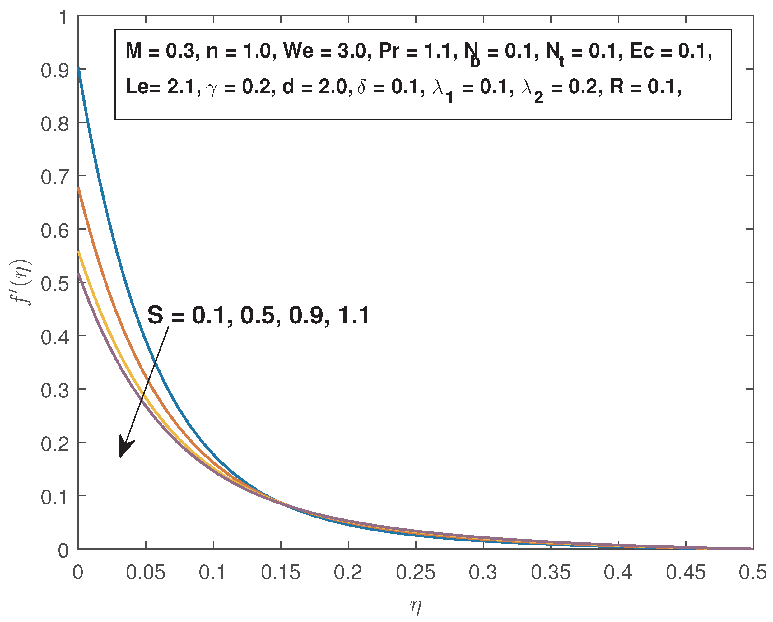
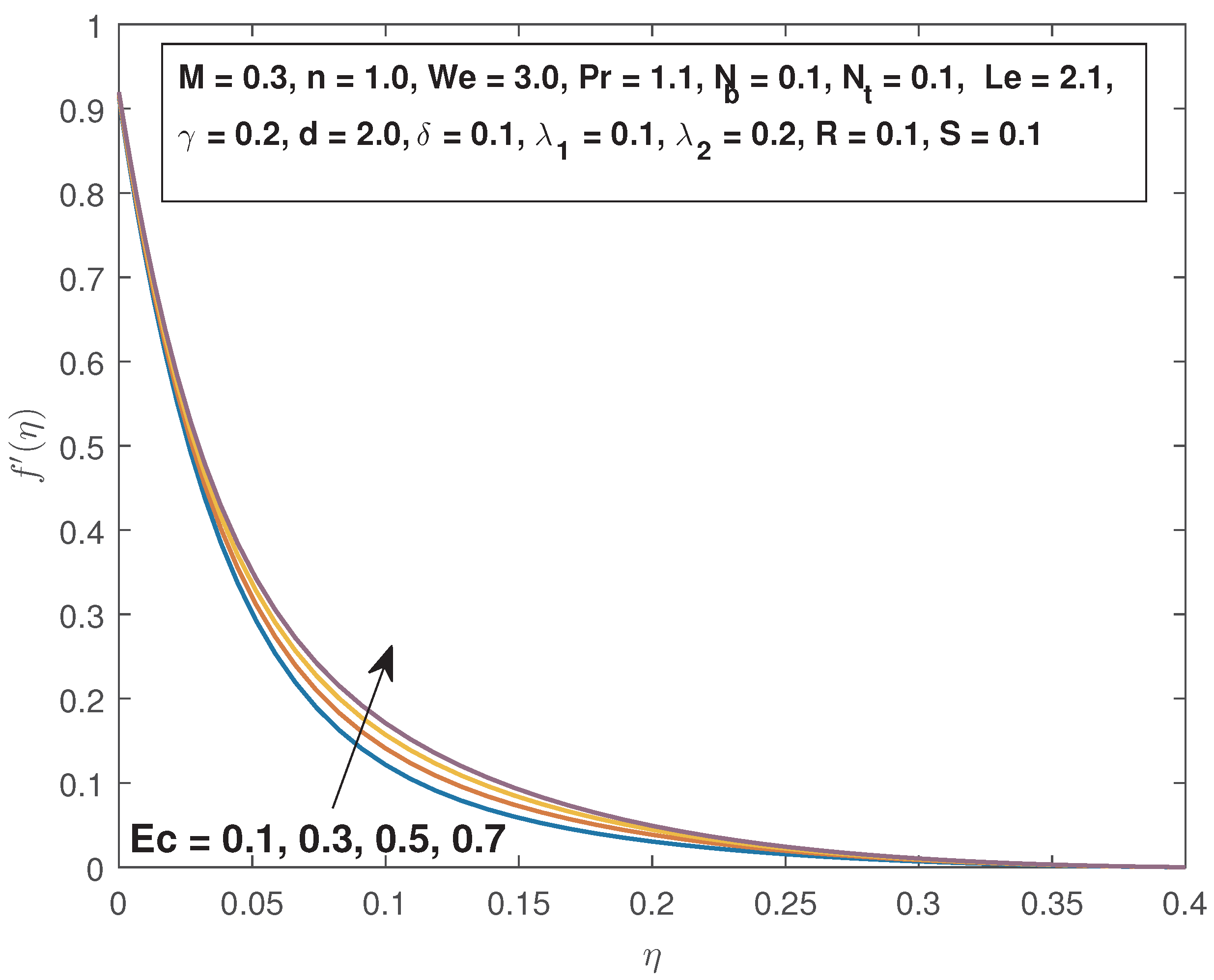
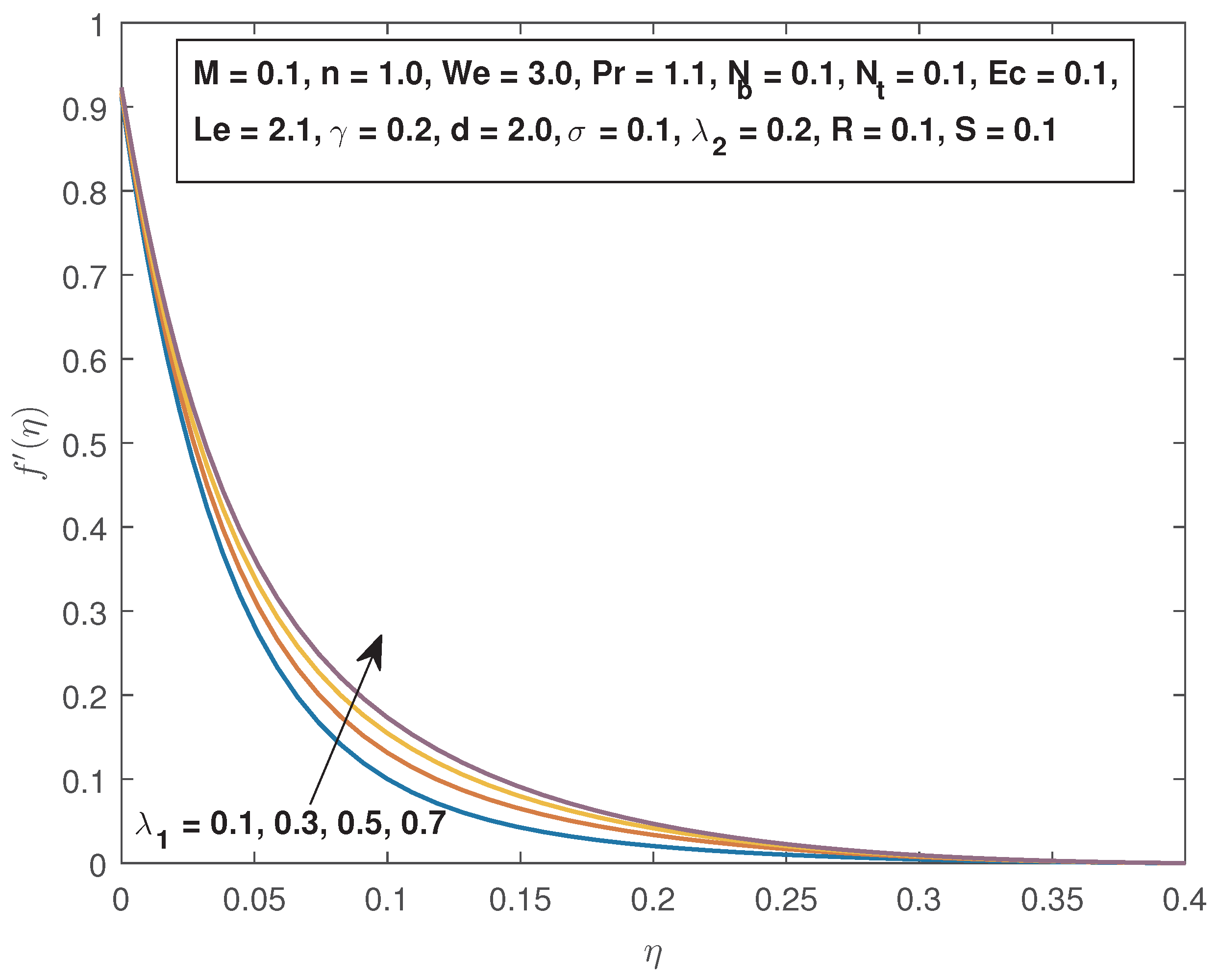
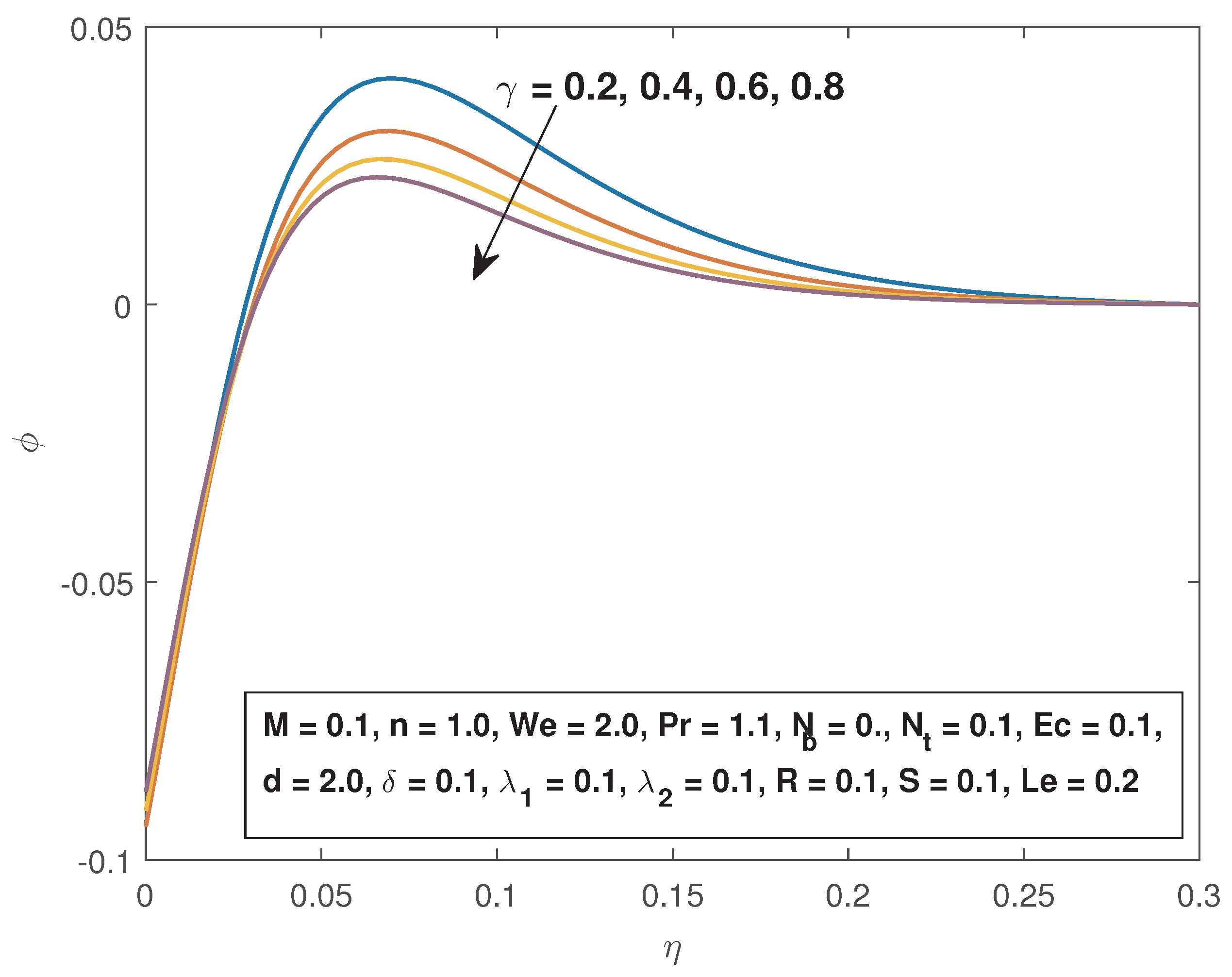
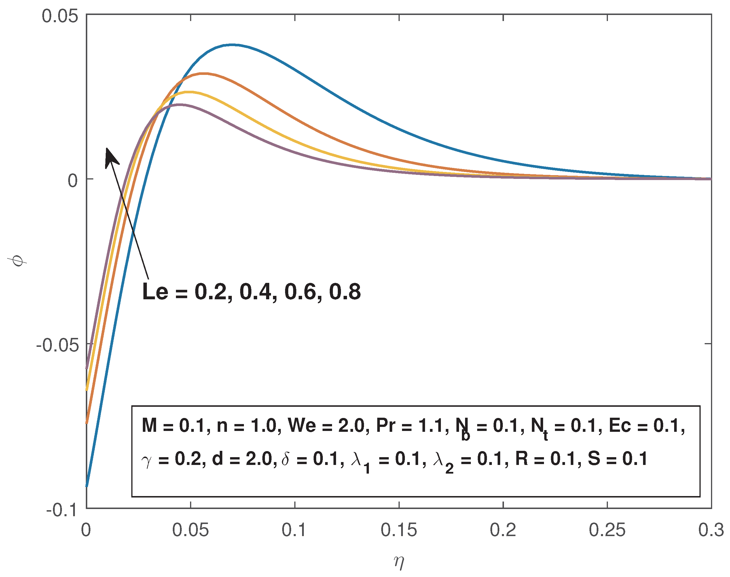
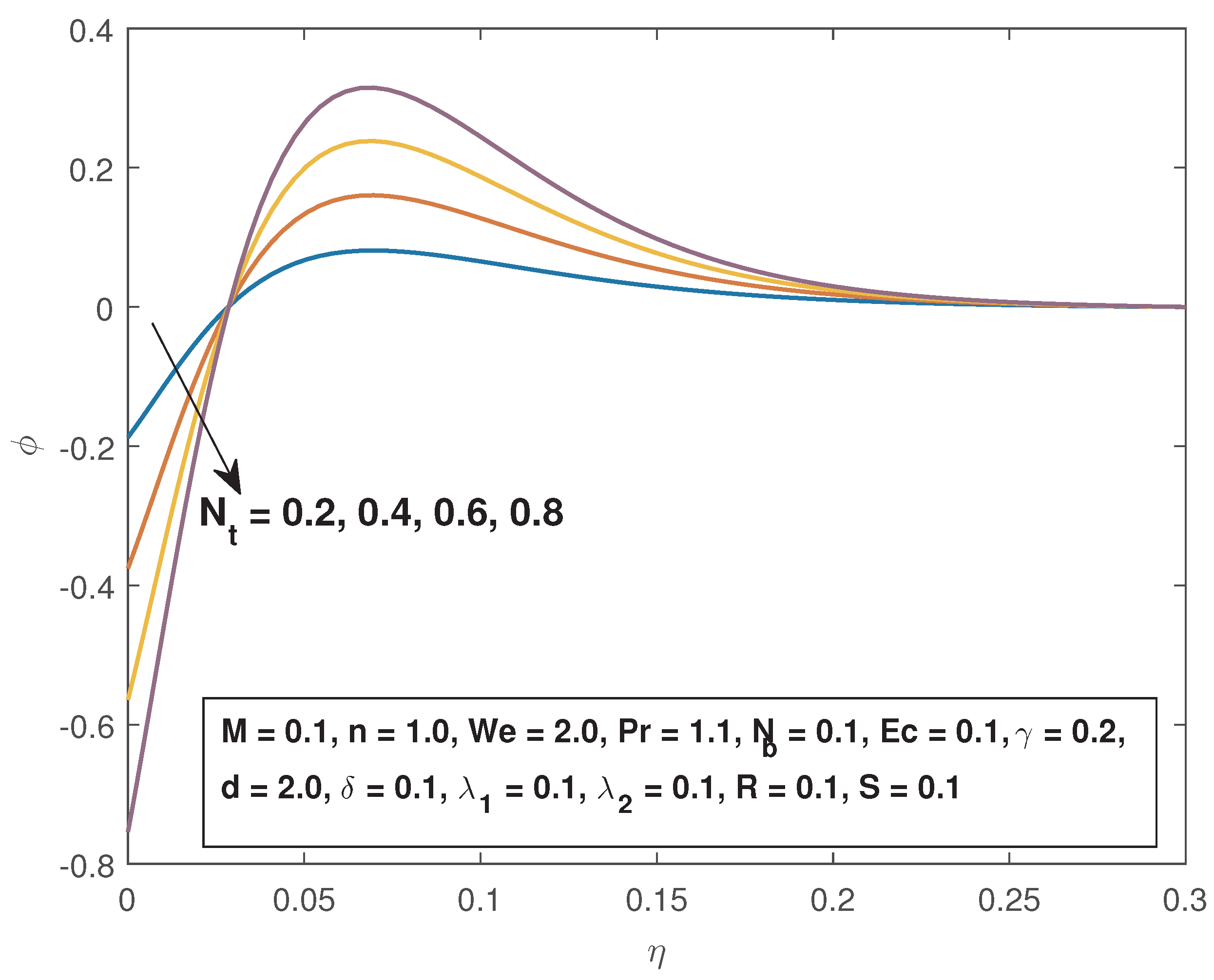
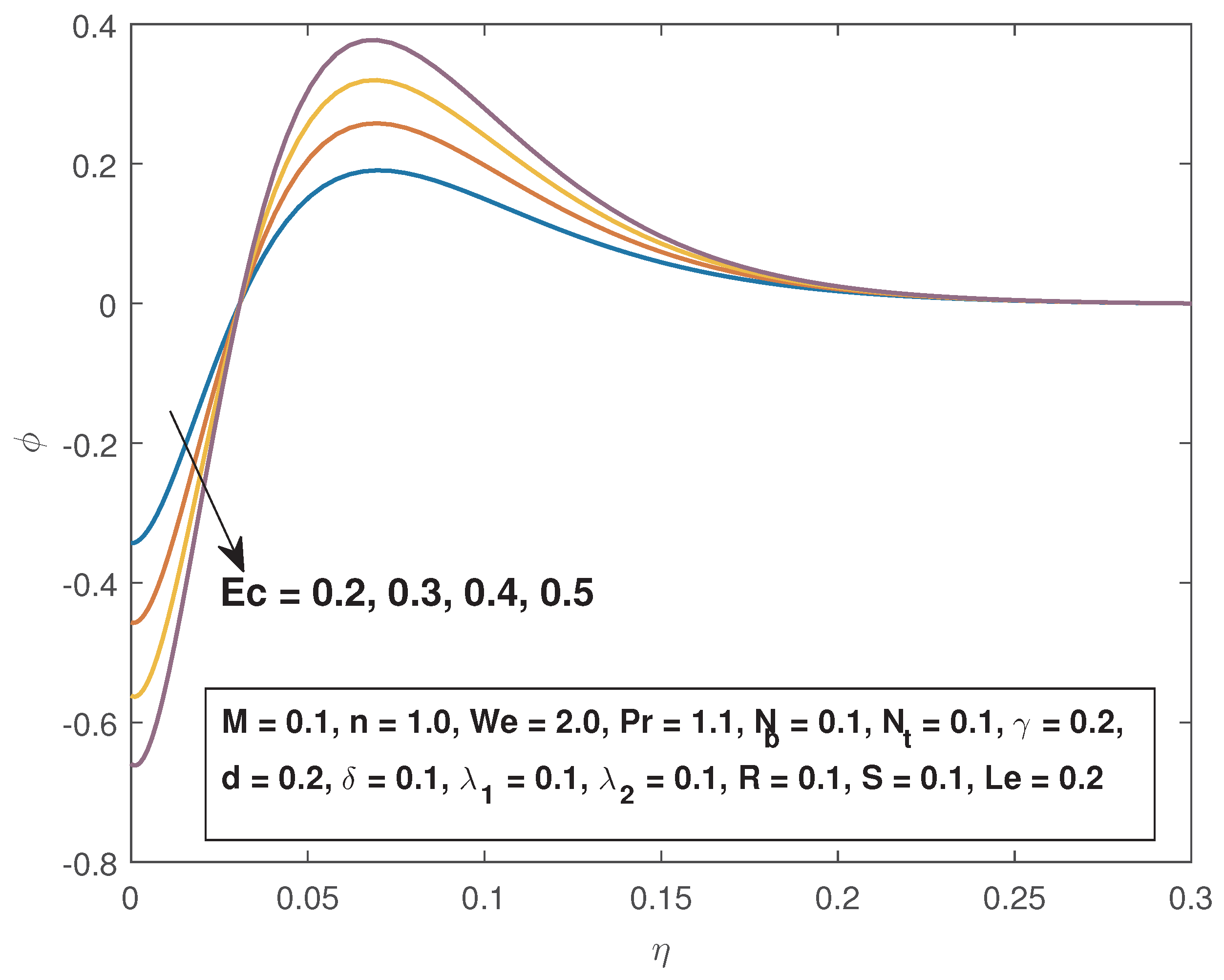
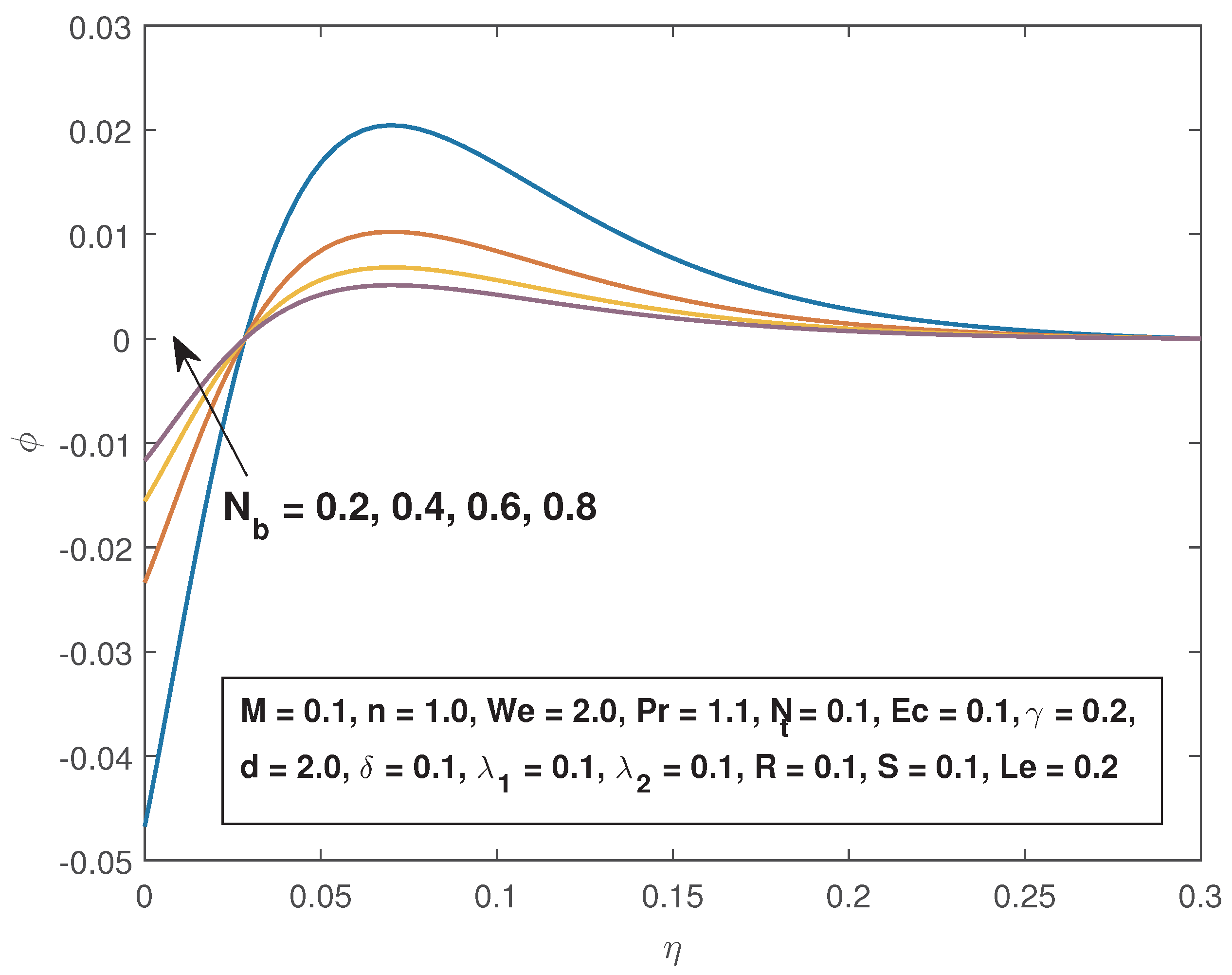
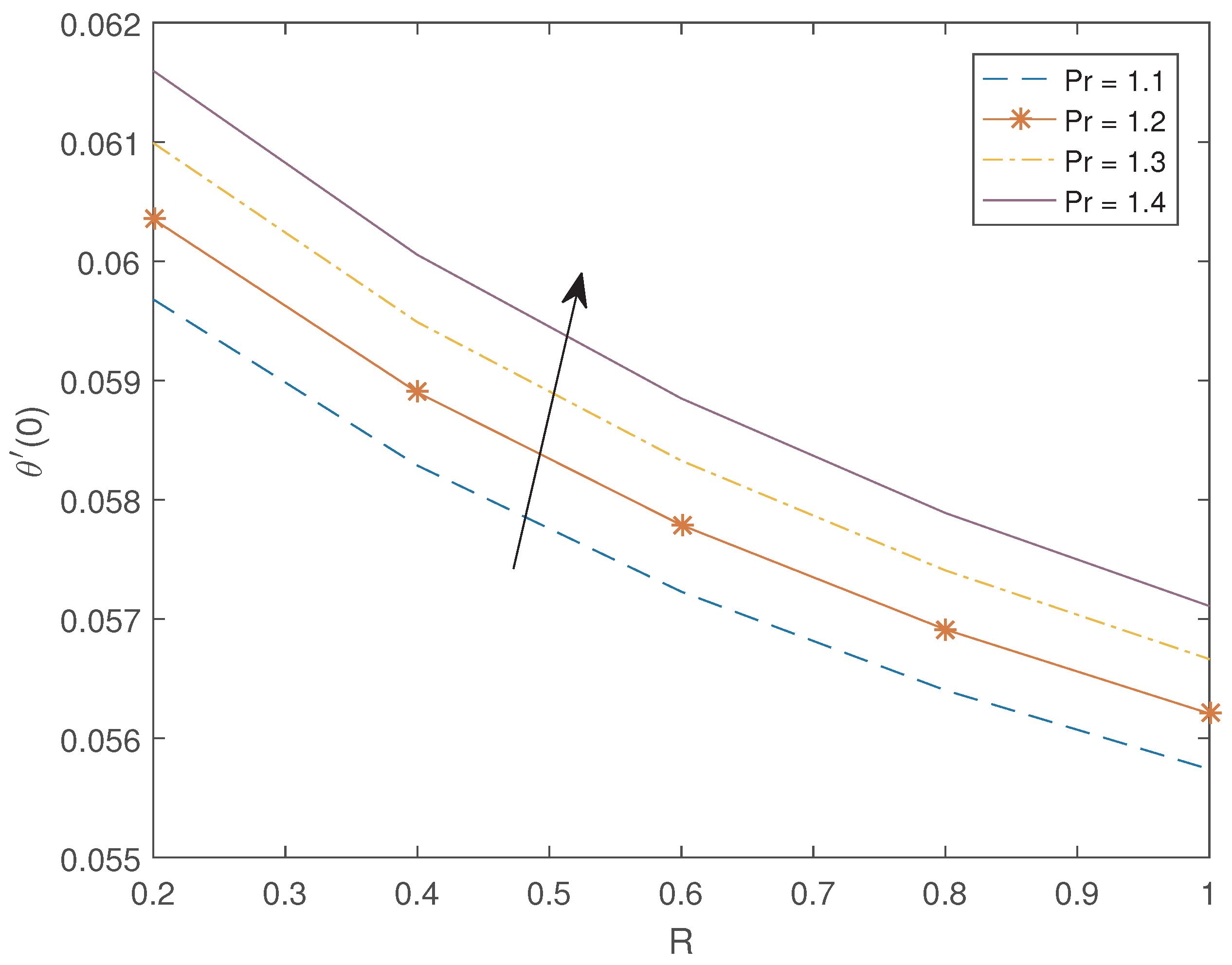
4. Results and Discussions

Discussed in this section are the numerical results of a coupled system of non-linear partial differential equations that model the Carreau–Yasuda nanofluid flow over a non-linearly stretching sheet in the presence of viscous dissipation and chemical reaction using SQLM. The linear system of Equations (28)–(30) together with boundary conditions (Equation (31)) is simplified using MATLAB 2016 (OPTI-NUM Solutions (Pty) Ltd, Johannesburg, South Africa). The influence of some physical parameters on the dimensionless velocity, temperature and concentration, the skin friction coefficient, the heat transfer rate and the mass transfer rate is shown by graphical representation. Tables are presented to portray the effects of some selected parameters on skin friction coefficient and the local Nusselt number.

Using $N=60$ collocation points in all the computations, solution-based errors were used to test for convergence of the numerical method. A solution-based error is the difference between two successive solutions, i.e., the solution at iteration level m and $m+1$. A plot of the infinity norms of the solution-based errors against the number of iterations is shown in Figure 2. A decrease of the error infinity norm with the number of iterations confirms the convergence of the method. The method converges after six iterations. Figure 3 is a plot of the residual error norms against the increasing number of iterations. It can be seen that there is a sharp decrease in the error as the number of iterations increases. This proves the high accuracy of the current method.

In all the numerical computations done in this work, the default parameters considered, unless otherwise stated, as in Khan et al. [15], are $M=0.3$, $n=1.0$, $We=3.0$, $Pr=1.1$, $N_b=0.1$, $N_t=0.1$, $E_c=0.1$, $Le=2.1$, $\gamma =0.2$, $d=2.0$, $\delta =0.1$, ${\lambda }_1=0.1$, ${\lambda }_2=0.2$, $R=0.1$, $S=0.1$.

Figure 4 shows the influence of the magnetic field parameter M on the nanofluid velocity. It is observed that when magnetic field parameter is enhanced, there is a decrease in the velocity distribution of the nanofluid. This is attributed to a Lorentz force that arise from the presence of a magnetic field that opposes the motion of the fluid and tends to resist the velocity, hence slowing down the fluid. The effect of the velocity slip parameter S on the fluid velocity is depicted in Figure 5. When the values of the slip velocity parameters are increased, the slip velocity increases and the fluid velocity decreases. Figure 6 reveals that enhancing the thermal slip parameter slightly increases the velocity profiles. The Eckert number relates the kinetic energy of the flow and the boundary layer enthalpy difference. As a result of viscous dissipation due to increased positive values of $Ec$, there will be an increased fluid initial temperature hence more thermal buoyancy effects that will induce more fluid flow. An increase in the values of $Ec$ results in an increase in the fluid velocity as shown in Figure 7. Figure 8 shows that increasing the thermal buoyancy parameter ${\lambda }_1$ increases the velocity of the nanofluid. Physically, increasing the thermal buoyancy creates a temperature difference in the flow that causes a reduction in the boundary layer and enhances the fluid velocity.

The effects of some thermophysical parameters namely the magnetic field parameter M, the Eckert number $Ec$, the thermal slip parameter $\delta$, the Prandtl number $Pr$, the thermal radiation parameter R, and the thermal buoyancy parameter ${\lambda }_1$ on the temperature profiles of the nanofluid are portrayed in Figure 9, Figure 10, Figure 11, Figure 12, Figure 13 and Figure 14. Figure 9 shows that increasing the magnetic field parameter increases the temperature of the nanofluid. Increasing the magnetic field parameter tends to reduce the fluid velocity profiles in the boundary and this will cause the thickening of the thermal boundary layer. The influence of $Ec$ on the temperature profiles is displayed in Figure 10. It is observed that increasing $Ec$ increases the temperature profiles. This is because of increased viscous dissipation due to internal friction. Figure 11 shows that increasing the thermal slip parameter has the effect of increasing the fluid temperature. The Prandtl number has an opposite effect to that of $\delta$ as shown in Figure 12. Increasing the values of $Pr$ is equivalent to a reducing thermal conductivity and hence a reduced thermal boundary layer. Figure 13 shows that increasing the thermal radiation parameter results in the increase in the temperature of the nanofluid. This due to the fact by increasing the radiation more heat energy is released to the flow thus enhancing temperature profiles. Increasing ${\lambda }_1$ depresses the temperature profiles as depicted in Figure 14.

The influence of the chemical reaction parameter $\gamma$, the Lewis number $Le$, $N_t$, $N_b$ and $Ec$ on the fluid concentration is shown in Figure 15, Figure 16, Figure 17 and Figure 18. As shown in Figure 15, the concentration profiles are decreased with an increase in the chemical reaction parameter. An increased chemical reaction causes the concentration boundary layer to thin due to a reduced chemical molecular diffusion hence a reduced mass diffusivity. The effect of the Lewis number $Le$ on the concentration of the nanofluid is reported in Figure 16. The Lewis number can be defined as the ratio of thermal diffusion rate to the species diffusion. For values $Le<1$, mass diffusion is rapid so the species boundary layer becomes thin. It is clear that increasing $Le$ causes an increase in the concentration profiles. Figure 17 and Figure 18 show that an increment in the $Nt$ and $Ec$ dwindles the concentration of the fluid. Figure 19 reveals that raising $Nb$ results in the concentration distribution and the identical boundary layer being increased.

Figure 20 depicts the effects of R through $N_t$ on the skin friction. By increasing $N_t(=0.1,0.3,0.5,0.7)$, the skin friction increases. The influence of the thermal radiation parameter R on the local Nusselt number for various values of the Prandtl number $Pr(=1.1,1.2,1.3,1.4)$ is displayed in Figure 21. This is evident because higher values of $Pr$ means the thickness of the thermal boundary layer decreases which in turn will result in an increase in wall temperature gradient. Also, an increase in thermal radiation parameter leads to an increased heat transfer rate. It is shown that the heat transfer rate is increased by increasing R and $Pr$. Figure 22 reports that increasing the magnetic field parameter M through the thermophoresis parameter $N_t(=0.1,0.3,0.5,0.7)$ enhances the local Sherwood number.

Table 1. Effects of selected parameters on the skin friction when $n=1.0$, $We=3.0$, $Pr=1.1$, $N_b=0.1$, $N_t=0.1$, $Le=2.1$, $\gamma =0.2$, $d=2.0$, $\delta =0.1$, ${\lambda }_2=0.2$, $R=0.1$.

M	${\mathit{E}}_{\mathit{c}}$	S	${\mathit{\lambda }}_1$	${\mathit{C}}_{\mathit{f}}{\mathit{Re}}_{\mathit{x}}^{-\frac{1}{2}}$
0.1	0.1	0.1	0.1	0.901165706578126
0.2	0.1	0.1	0.1	0.939430977283166
0.3	0.1	0.1	0.1	0.975901612948121
0.1	0.1	0.1	0.1	0.901165706578126
0.1	0.3	0.1	0.1	0.894342142778385
0.1	0.5	0.1	0.1	0.887855032025925
0.1	0.1	0.1	0.1	0.901165706578126
0.1	0.1	0.5	0.1	0.607698358897778
0.1	0.1	0.9	0.1	0.465481562823527
0.1	0.1	0.1	0.1	0.901165706578126
0.1	0.1	0.1	0.3	0.877937713382835
0.1	0.1	0.1	0.5	0.856014644415950

and

Table 2. The values of $N{u}_{x}R{e}_x^{-\frac{1}{2}}$ for different values of selected parameters when $n=1.0$, $We=3.0$, $M=0.3$, $N_b=0.1$, ${\lambda }_1=0.1$, $E_c=0.1$, $Le=2.1$, $\gamma =0.2$, $d=2.0$, $E_c=0.1$, ${\lambda }_2=0.2$, $S=0.1$.

$\mathit{Pr}$	$\mathit{\delta }$	R	${\mathit{N}}_{\mathit{t}}$	$\mathbf{-}{\mathit{Nu}}_{\mathit{x}}{\mathit{Re}}_{\mathit{x}}^{\frac{\mathbf{1}}{\mathbf{2}}}$
1.1	0.1	0.1	0.1	0.078548380963099
1.2	0.1	0.1	0.1	0.079117794840876
1.3	0.1	0.1	0.1	0.079609418569888
1.1	0.1	0.1	0.1	0.078548380963099
1.1	0.3	0.1	0.1	0.179932397357334
1.1	0.5	0.1	0.1	0.242732064006873
1.1	0.1	0.1	0.1	0.078548380963099
1.1	0.1	0.3	0.1	0.077003538347739
1.1	0.1	0.5	0.1	0.075588054175029
1.1	0.1	0.1	0.1	0.078548380963099
1.1	0.1	0.1	0.3	0.077003538347739
1.1	0.1	0.1	0.5	0.075588054175029

depict the effects of some selected parameters on the skin friction coefficient and heat transfer rate, respectively. From Table 1, we can infer that the skin friction coefficient is significantly and slightly increased by increasing the magnetic field parameter M and the Eckert number $Ec$, respectively. The table also shows that the slip velocity S heavily depress the skin friction coefficient. Increasing the thermal buoyancy parameter slightly decreases the skin friction coefficient. Table 2 reflects that increasing the thermal slip parameter $\delta$ and the Prandtl number $Pr$ enhances the local Nusselt number $N{u}_{x}R{e}_x^{-\frac{1}{2}}$.

5. Conclusions

This paper considers the Carreau–Yasuda nanofluid flow over a non-linear stretching sheet. The effects of viscous dissipation and chemical reaction were taken into account. The system of coupled non-linear partial differential equation describing the model were transformed into a coupled system of linear differential equations using a suitable similarity transformation. The resulting linear differential equations were numerically solved using the spectral quasi-linearization method. The convergence and accuracy of the SQLM was determined by the error infinity norms and the residual error infinity norms, respectively. Key findings from this study are the following:

• The spectral quasi-linearization method is a very efficient and reliable method for solving non-linear differential equations.
• The fluid velocity and the momentum boundary layer increase with increasing Eckert number, thermal buoyancy parameter, thermal slip parameter, and decrease with the magnetic field parameter, and the velocity slip parameter.
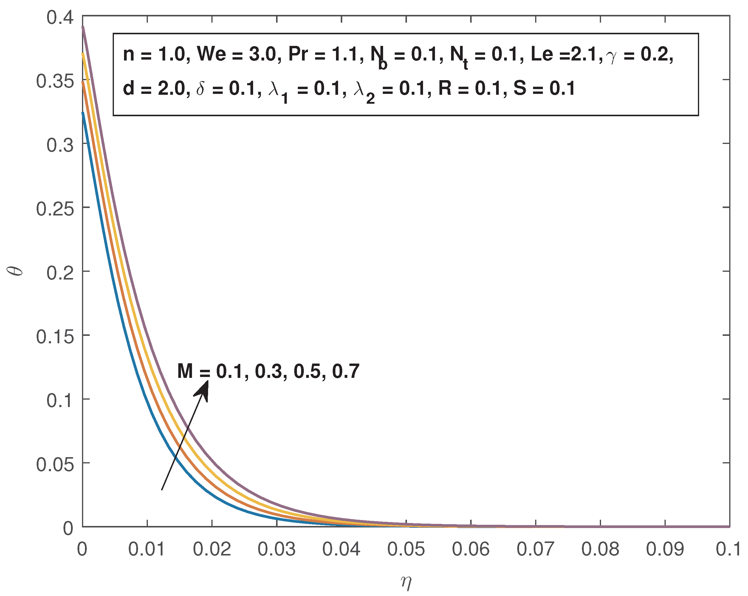
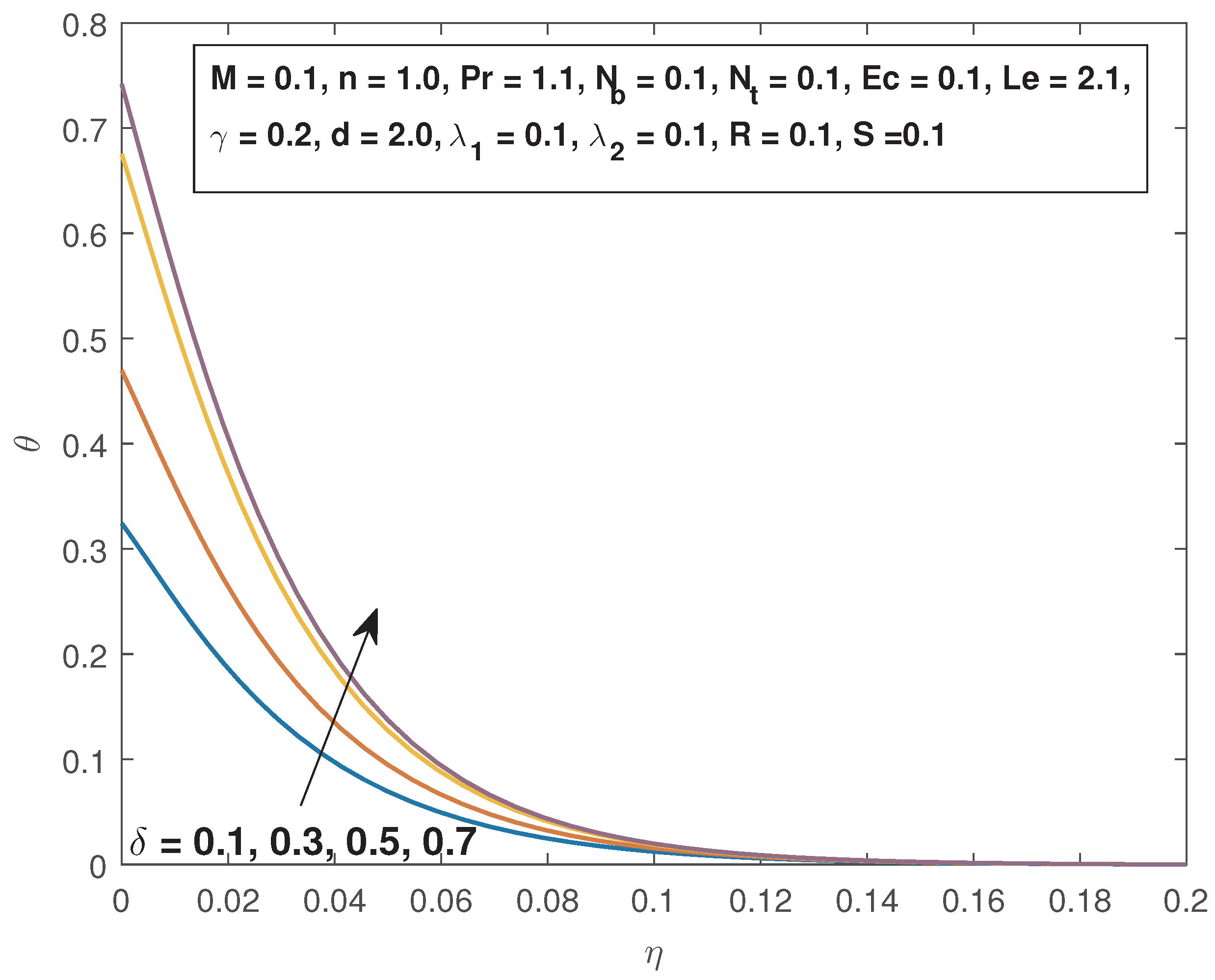
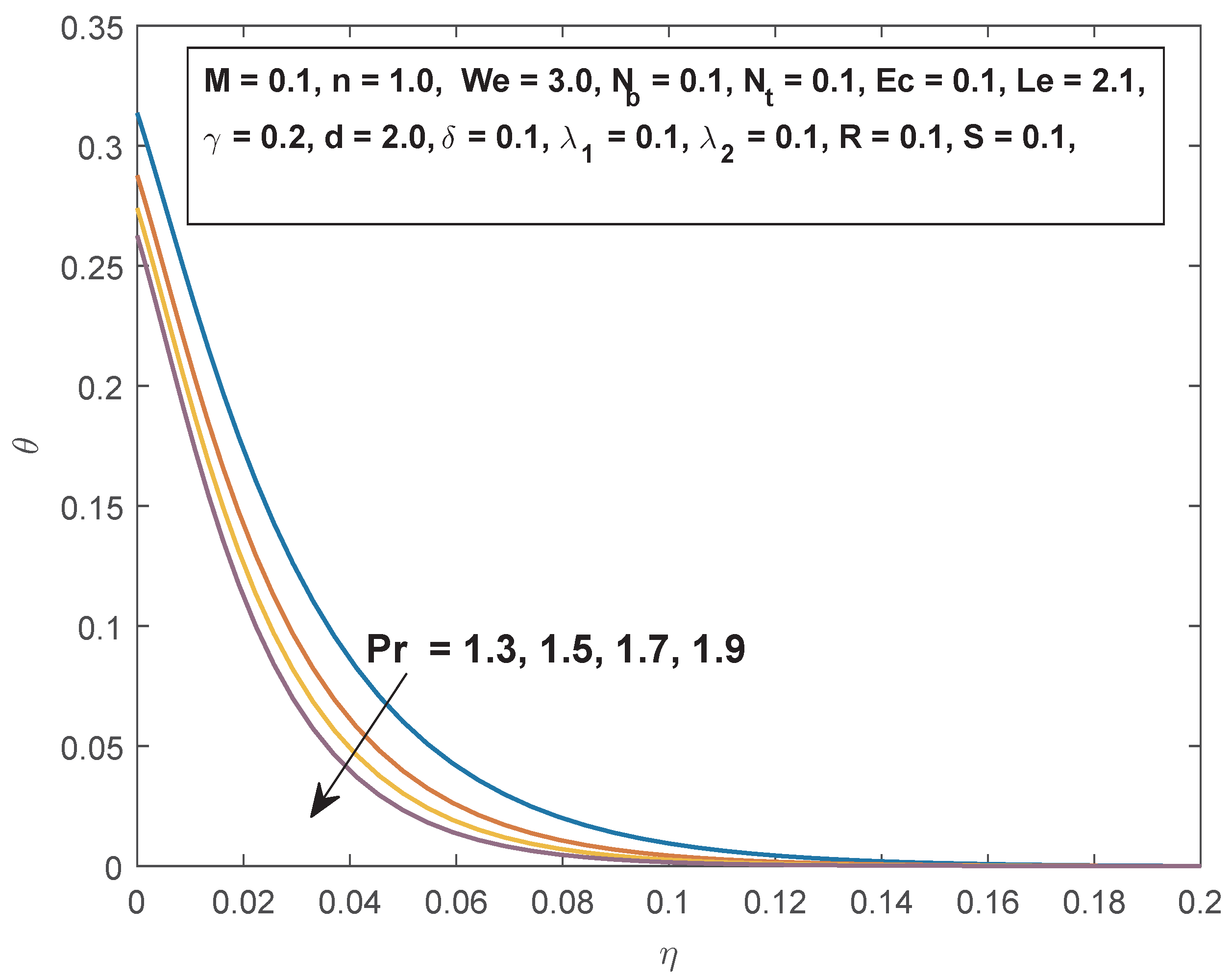
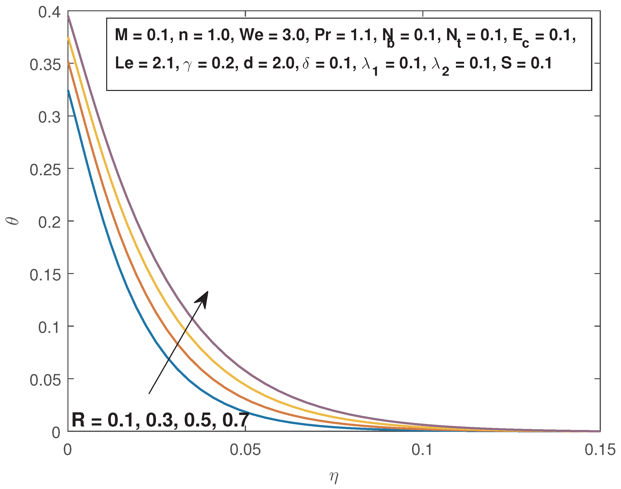
• The fluid temperature increases with increasing magnetic field parameter, Eckert number, thermal slip parameter, and the thermal radiation parameter, and is decreased by raising the Prandtl number and thermal buoyancy parameter.
• The fluid concentration in enhanced by increasing the Lewis number and the Brownian motion parameter while it is depressed by increased thermal reaction parameter, thermophoresis parameter and the Eckert number.
• The skin friction is increases with increasing magnetic field parameter and decreases when the Eckert number, thermal buoyancy parameter and the velocity slip parameter are increased.
• The local Nusselt number increases when the Prandtl number and the thermal slip parameter are increased, while the opposite trend is observed when thermal radiation parameter and thermophoresis parameter are increased.

References

1. Kahshan, M.; Lu, D.; Rahimi-Gorji, M. Hydrodynamical study of flow in a permeable channel: Application to flat plate dialyzer. Int. J. Hydrogen Energy 2019. [Google Scholar] [CrossRef]
2. Cioranescu, D.; Girault, V.; Rajagopal, K.R. Mechanics and Mathematics of Fluids of the Differential Type. Adv. Mech. Math. 2016. [Google Scholar] [CrossRef]
3. Kheyfets, V.O.; Kieweg, S.L. Gravity-driven thin film flow of anEllis fluid. J. Nonnewton Fluid Mech. 2013, 202, 88–98. [Google Scholar] [CrossRef] [PubMed] [Green Version]
4. Sochi, T. Analytical solutions for the flow of Carreau and Cross fluids in circular pipes and thin slits. Rheol. Acta 2015, 54, 745–756. [Google Scholar] [CrossRef] [Green Version]
5. Hina, S.; Hayat, T.; Asghar, S.; Hendi, A.A. Influence of compliant walls on peristalic motion with heat/mass transfer and chemical reaction. Int. J. Heat Mass Trans. 2012, 55, 3386–3394. [Google Scholar] [CrossRef]
6. Mekheimer, K.S.; Abd Elmaboud, Y. Simultaneous effects of variable viscosity and thermal conductivity on peristaltic flow in a vertical asymmetric channel. Can. J. Phys. 2014, 92, 1541–1555. [Google Scholar] [CrossRef]
7. Mahmood, R.; Bilal, S.; Khan, I.; Kousar, N.; Seikh, A.H.; El-Sayed, M.S. A comprehensive finite element examination of Carreau Yasuda fluid model in a lid driven cavity and channel with obstacle by way of kinetic energy and drag and lift coefficient measurements. J. Mater. Res. Technol. 2019. [Google Scholar] [CrossRef]
8. Andrade, L.C.F. The Carreau-Yasuda Fluids: A skin friction equation for turbulent flow in pipes and Kolmogorov dissipative scales. J. Braz. Soc. Mech. Sci. Eng. 2007, 29, 162–167. [Google Scholar] [CrossRef]
9. Hayat, T.; Abbasi, F.M.; Ahmad, B.; Alsaedi, A. Peristaltic Transport of Carreau-Yasuda Fluid in a Curved Channel with Slip Effects. PLoS ONE 2014, 9, e95070. [Google Scholar] [CrossRef]
10. Hayat, T.; Asad, S.; Mustafa, M.; Alsaedi, A. Boundary layer flow of Carreau fluid over a convectively heated stretching. Appl. Math. Comput. 2014, 245, 12–22. [Google Scholar] [CrossRef]
11. Abbasi, F.M.; Hayat, T.; Alsaedi, A. Numerical analysis for MHD peristaltic transport of Carreau–Yasuda fluid in a curved channel with Hall effects. J. Magnet. Magnet. Mater. 2015, 382, 104–110. [Google Scholar] [CrossRef]
12. Shamekhi, A.; Sadeghy, K. Cavity flow simulation of Carreau–Yasuda non-Newtonian fluids using PIM meshfree method. Appl. Math. Model. 2009, 33, 4131–4145. [Google Scholar] [CrossRef]
13. Lashgari, L.; Pralits, J.O.; Giannetti, F.; Brandt, I. First instability of the flow of shear-thinning and shear-thickening fluids past a circular cylinder. J. Fluid Mech. 2012, 701, 201–227. [Google Scholar] [CrossRef] [Green Version]
14. Zhao, J.; Zheng, L.; Zhang, X. Mixed Convection Heat Transfer of Non-newtonian Carreau–Yasuda Fluid Driven by Power Law Temperature Gradient. Heat Transf. Res. 2017, 48, 849–864. [Google Scholar] [CrossRef]
15. Khan, M.; Shahid, A.; Malik, M.Y.; Salahuddin, T. Chemical reaction for Carreau-Yasuda nanofluid flow past a nonlinear stretching sheet considering Joule heating. Results Phy. 2018, 8, 1124–1130. [Google Scholar] [CrossRef]
16. Salahuddin, T.; Malik, M.Y.; Hussain, A.; Bilal, S.; Awais, M.; Khan, I. MHD squeezed flow of Carreau-Yasuda fluid over a sensor surface. Alexandria Eng. J. 2017, 56, 27–34. [Google Scholar] [CrossRef] [Green Version]
17. Hayat, T.; Aslam, N.; Khan, M.I.; Alsaedi, A. Mixed convective peristaltic flow of Carreau–Yasuda fluid in an inclined symmetric channel. Microsyst. Technol. 2019, 25, 609–620. [Google Scholar] [CrossRef]
18. Migtaa, H.M.; Al- Khafajy, D.G.S. Influence of Heat Transfer on Magnetohydrodynamics Oscillatory Flow for Carreau-Yasuda Fluid Through a Porous Medium. J. Al-Qadisiyah Comput. Sci. Math. 2019, 11, 76–88. [Google Scholar]
19. Choi, S.U.S.; Eastman, J.A. Enhancing thermal conductivity of fluids with nanoparticles. In Proceedings of the 1995 International mechanical engineering congress and exhibition, San Francisco, CA, USA, 12–17 November 1995; pp. 99–105. [Google Scholar]
20. Nandkeolyar, R.; Mahatha, B.K.; Mahato, G.K.; Sibanda, P. Effect of Chemical Reaction and Heat Absorption on MHD Nanoliquid Flow Past a Stretching Sheet in the Presence of a Transverse Magnetic Field. Magnetochemistry 2018, 4, 18. [Google Scholar] [CrossRef] [Green Version]
21. Anuar, N.S.; Bachok, N. Blasius and Sakiadis problems in nano-fluids using Buongiorno model and thermo-physical properties of nano-liquids. Eur. Int. J. Sci. Technol. 2016, 5, 65–81. [Google Scholar]
22. Prakash, D.; Suriyakumar, P. Transient hydromagnetic convection flow of nanofluid between asymmetric vertical plates with heat generation. Int. J. Pure Appl. Math. 2017, 113, 1–10. [Google Scholar]
23. Sharma, R.; Hussain, S.D.; Joshi, H.; Sethi, G.S. Analysis of radiative magneto-nanofluid over an accelerated plate in a rotating medium with Hall effects. Differ. Found. 2017, 11, 129–145. [Google Scholar] [CrossRef]
24. Astuti, A.; Sri, P.; Kaprawi, S. Natural Convection of Nanofluids past an Accelerated Vertical Plate with Variable Wall Temperature by Presence of the Radiation. Front. Heat Mass Transfer (FHMT) 2019, 13, 3. [Google Scholar] [CrossRef] [Green Version]
25. Hady, F.M.; Ibrahim, F.S.; Abdel-Gaied, S.M.; Eid, M.R. Radiation effect on viscous flow of a nanofluid and heat transfer over a nonlinearly stretching sheet. Nanoscale Res. Lett. 2012, 7, 1–13. [Google Scholar] [CrossRef] [PubMed] [Green Version]
26. Shateyi, S.; Prakask, J. A new numerical approach for MHD laminar boundary layer flow and heat transfer of nanofluids over a moving surface in the presence of thermal radiation. Bound. Value Prob. 2014, 2. [Google Scholar] [CrossRef] [Green Version]
27. Krishnamurthy, M.R.; Gireesha, B.J.; Prasannakumara, B.C.; Gorla, R.S.R. Thermal radiation and chemical reaction effects on boundary layer slip flow and melting heat transfer of nanofluid induced by a nonlinear stretching sheet. Nonlinear Eng. 2016, 5, 147–159. [Google Scholar] [CrossRef]
28. Elbashbeshy, E.M.A.; Emam, T.G. Effects of Thermal Radiation and Heat Transfer over an Unsteady Stretching Surface Embedded in a Porous Medium in the Presence of Heat Source or Sink. Therm. Sci. 2011, 15, 477–485. [Google Scholar]
29. Khan, I.; Shafquatullah, M.Y.; Malik, M.Y.; Hussain, A.; Khan, M. Magnetohydrodynamics Carreau nanofluid flow over an inclined convective heated stretching cylinder with joule heating. Results Phys. 2017, 7, 4001–4012. [Google Scholar] [CrossRef]
30. Cheng, K.C.; Wu, R.S. Viscous Dissipation Effects on Convective Instability and Heat Transfer in Plane Poiseuille Flow Heated from Below. Appl. Sci. Res. 1976, 32, 327–346. [Google Scholar] [CrossRef]
31. Boubaker, K.; Li, B.; Zheng, L.; Bhrawy, A.H.; Zhang, X. Effects of Viscous Dissipation on the Thermal Boundary Layer of Pseudoplastic Power-Law Non-Newtonian Fluids Using Discretization Method and the Boubaker Polynomials Expansion Scheme. ISRN Therm. 2012, 2012, 181286. [Google Scholar] [CrossRef] [Green Version]
32. Lund, L.A.; Omar, Z.; Khan, I.; Kadry, S.; Rho, S.; Mari, I.A.; Nisar, K.S. Effect of Viscous Dissipation in Heat Transfer of MHD Flow of Micropolar Fluid Partial Slip Conditions: Dual Solutions and Stability Analysis. Energies 2019, 12, 4617. [Google Scholar] [CrossRef] [Green Version]
33. Motsa, S.S.; Dlamini, P.G.; Khumalo, M. Spectral Relaxation Method and Spectral Quasilinearization Method for Solving Unsteady Boundary Layer Flow Problems. Adv. Math. Phys. 2014, 2014, 1–12. [Google Scholar] [CrossRef]
34. Alharbey, R.A.; Mondal, H.; Behl, R. Spectral Quasi-Linearization Method for Non-Darcy Porous Medium with Convective Boundary Condition. Entropy 2019, 21, 838. [Google Scholar] [CrossRef] [Green Version]
35. Pal, D.; Mondal, S.; Mondal, H. Entropy generation on MHD Jeffrey nanofluid over a stretching sheet with nonlinear thermal radiation using spectral quasilinearization Method. Int. J. Ambient Energy 2019, 1–24. [Google Scholar] [CrossRef]
36. Das, S.; Mondal, H.; Kundu, P.K.; Sibanda, P. Spectral quasi-linearization method for Casson fluid with homogeneous heterogeneous reaction in presence of nonlinear thermal radiation over an exponential stretching sheet. Multidiscip. Model. Mater. Struct. 2018. [Google Scholar] [CrossRef]
37. Shateyi, S.; Muzara, H. On the Numerical Analysis of Unsteady MHD Boundary Layer Flow of Williamson Fluid Over a Stretching Sheet and Heat and Mass Transfers. Computation 2020, 8, 55. [Google Scholar] [CrossRef]
38. Bellman, R.E.; Kalaba, R.E. Quasilinearization and Nonlinear Boundary-Value Problems; Elsevier: New York, NY, USA, 1965. [Google Scholar]
39. Trefethen, L.N. Spectral Methods in MATLAB; SIAM: Philadelphia, PA, USA, 2000. [Google Scholar]
Figure 1. Flow configuration and coordinate system.
Mathematics 08 01148 g001
Figure 2. Convergence graphs of f ( η ) , θ ( η ) and ϕ ( η ) .
Mathematics 08 01148 g002
Figure 3. Accuracy graphs of f ( η ) , θ ( η ) and ϕ ( η ) .
Mathematics 08 01148 g003
Figure 4. Influence of M on the fluid velocity.
Mathematics 08 01148 g004
Figure 5. Influence of S on the fluid velocity.
Mathematics 08 01148 g005
Figure 6. Effects of δ on the fluid velocity.
Mathematics 08 01148 g006
Figure 7. Effects of E c on the fluid velocity.
Mathematics 08 01148 g007
Figure 8. Influence of λ 1 on the fluid velocity.
Mathematics 08 01148 g008
Figure 9. Influence of M on the fluid temperature.
Mathematics 08 01148 g009
Figure 10. Influence of E c on the fluid temperature.
Mathematics 08 01148 g010
Figure 11. Influence of δ on the fluid temperature.
Mathematics 08 01148 g011
Figure 12. Influence of P r on the fluid temperature.
Mathematics 08 01148 g012
Figure 13. Influence of R on the fluid temperature.
Mathematics 08 01148 g013
Figure 14. Influence of λ 1 on the fluid temperature.
Mathematics 08 01148 g014
Figure 15. Influence of γ on the fluid concentration.
Mathematics 08 01148 g015
Figure 16. Influence of L e on the fluid concentration.
Mathematics 08 01148 g016
Figure 17. Influence of N t on the fluid concentration.
Mathematics 08 01148 g017
Figure 18. Influence of E c on the fluid concentration.
Mathematics 08 01148 g018
Figure 19. Influence of N b on the fluid concentration.
Mathematics 08 01148 g019
Figure 20. Influence of R and N t on the skin friction.
Mathematics 08 01148 g020
Figure 21. Influence of R and P r on the heat transfer rate.
Mathematics 08 01148 g021
Figure 22. Influence of M and N t on the mass transfer.
Mathematics 08 01148 g022