Abstract
Modeling insurance data using heavy-tailed distributions is of great interest for actuaries. Probability distributions present a description of risk exposure, where the level of exposure to the risk can be determined by “key risk indicators” that usually are functions of the model. Actuaries and risk managers often use such key risk indicators to determine the degree to which their companies are subject to particular aspects of risk, which arise from changes in underlying variables such as prices of equity, interest rates, or exchange rates. The present study proposes a new heavy-tailed exponential distribution that accommodates bathtub, upside-down bathtub, decreasing, decreasing-constant, and increasing hazard rates. Actuarial measures including value at risk, tail value at risk, tail variance, and tail variance premium are derived. A computational study for these actuarial measures is conducted, proving that the proposed distribution has a heavier tail as compared with the alpha power exponential, exponentiated exponential, and exponential distributions. We adopt six estimation approaches for estimating its parameters, and assess the performance of these estimators via Monte Carlo simulations. Finally, an actuarial real data set is analyzed, proving that the proposed model can be used effectively to model insurance data as compared with fifteen competing distributions.
1. Introduction
Heavy-tailed distributions have been used in modeling data in several applied areas such as risk management, economic, and actuarial sciences. The insurance data sets are usually positive (Klugman et al. [1]), unimodal shaped (Cooray and Ananda [2]), right-skewed (Lane [3]), and with heavy tails (Ibragimov and Prokhorov [4]). Right-skewed data may be adequately modeled by skewed distributions (Bernardi et al. [5]). Modeling insurance data using heavy-tailed distributions is of a great interest for actuaries. Furthermore, actuaries and risk managers are often interested in “the chance of an adverse outcome”, which can be expressed through the value at risk (VaR) at a particular probability level. The VaR can also be utilized to determine the amount of capital required to withstand such adverse outcomes. Investors and rating agencies are particularly interested in the company’s ability to withstand such events.
Hence, several unimodal positively skewed distributions are utilized to model such data sets (Adcock et al. [6] and Bhati and Ravi [7]).
The heavy-tailed distributions have right tail probabilities which are heavier than the exponential one, that is, for any baseline with cumulative distribution function (CDF) , we have
More information about heavy-tailed distributions can be found in Resnick [8] and Beirlant et al. [9].
An empirical analysis for loss distributions to estimate the risk using some approaches is conducted by Dutta and Perry [10], who pointed out that the exponential, gamma, and Weibull models can not be used because of their poor results and stated that one would need to use a more flexible model. There are some methods that have been introduced to construct new distributions with heavier tails than the exponential distribution, called the transformation method, compounding of distributions, composition of two or more models and finite mixture distributions. The interested reader can refer to Eling [11], Kazemi and Noorizadeh [12], Bakar et al. [13], Punzo [14], Mazza and Punzo [15], Miljkovic and Grun [16], and Punzo et al. [17].
Aforementioned approaches may be very useful in constructing more flexible distributions; however, these methods are still subject to some sort of deficiencies, such as the inferences of transformation approach become difficult and require much computational work to derive the distributional characteristics (see Bagnato and Punzo [18]), and the approach of composition of two or more models based on fixed or pre-defined mixing weights, may be very restrictive (see Calderin-Ojeda and Kwok [19]).
Hence, it is important to develop more flexible models either from the existing classical distributions or a new class of distributions to model different insurance data including insurance loss data, unemployment insurance data, and financial returns, among others. In the present paper, we are motivated to propose a more flexible distribution called alpha power exponentiated exponential (APExE) distribution, which provides greater accuracy and flexibility in fitting actuarial data.
Furthermore, the aim of the paper is three-fold: first to study a new extension of the exponential (E) and exponentiated exponential (ExE) distributions based on an alpha power-G (AP-G) family proposed by Mahdavi and Kundu [20], called the APExE distribution. Some distributional properties of the APExE distribution are derived. The proposed model has some desirable properties such as
- The APExE model contains, as special cases, some lifetime distributions, called E, ExE [21], and alpha power exponential (APE) [20] distributions.
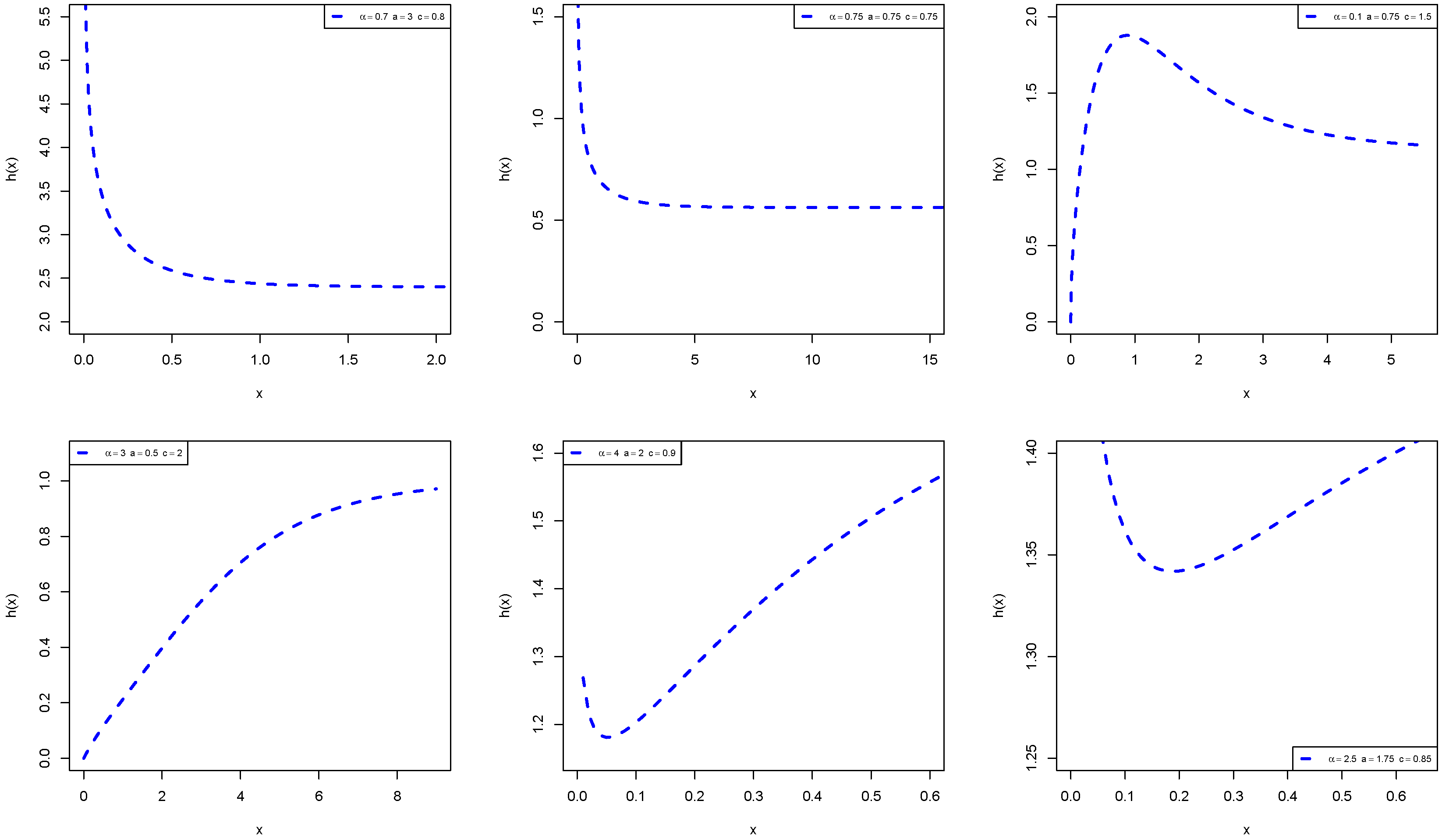
- The APExE distribution accommodates upside down bathtub, bathtub, decreasing, decreasing-constant and increasing hazard rates, and right-skewed, symmetrical, left-skewed, J-shape, reversed-J shape, and unimodal densities (see Figure 1 and Figure 2).

 Figure 1. Plots of APExE PDFs for different parametric values.
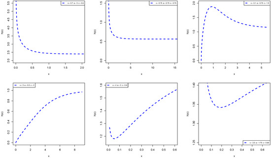 Figure 2. Plots of APExE HRF for different parametric values.
 - It provides a heavier tailed distribution than the APE, ExE, and E distributions based on computational results of risk measures (see also Section 4).
- The APExE has closed forms for its CDF and hazard rate function (HRF). Hence, it can be used conveniently in analyzing censored data. Furthermore, it can be used to model various data in actuarial applications.
- It can be utilized to model heavy-tailed insurance data from actuarial science than other competing models. The proposed APExE distribution provides better fits than other fifteen competing distributions in modeling unemployment insurance data (see Section 7).
One of the most important subjects of actuarial sciences is to evaluate the exposure to market risk in a portfolio of instruments, which arise from changes in underlying variables such as prices of equity, interest rates, or exchange rates. Hence, our second objective is to derive some important risk or actuarial measures including VaR, tail value at risk (TVaR), tail variance (TV), and tail variance premium (TVP) for the APExE distribution, which play a crucial role in portfolio optimization under uncertainty. Third, we explore the estimation of the APExE parameters by six methods of estimation. Such methods include the maximum likelihood estimators (MLE), ordinary least-squares estimators (OLSE), weighted least squares estimators (WLSE), Anderson–Darling estimators (ADE), Cramér–von Mises estimators (CVME), and percentile estimators (PE). We compare these estimators using an extensive computational study in order to develop a guideline for choosing the best method of estimation that provides better estimates for the APExE parameters, which we think would be of a great interest to applied actuaries/statisticians/engineers.
The paper is organized as follows. In Section 2, we define the APExE distribution. Its mathematical properties are derived in Section 3. In Section 4, we discuss four important actuarial measures based on the APExE distribution and present some numerical results for them. Six methods of parameter estimation are explored in Section 5. The performance of estimation methods is adopted by simulation results in Section 6. In Section 7, we consider a heavy-tailed real data set from the insurance field to illustrate the usefulness of the APExE distribution. Final remarks are presented in Section 8.
2. The APExE Distribution
In this section, we present the APExE model that can be specified by the following CDF and probability density function (PDF)
where is a scale parameter and , and are shape parameters. By setting , the APExE reduces to APE distribution (Mahdavi and Kundu [20]). The ExE distribution (Gupta and Kundu [21]) follows from the APExE distribution with , whereas the E follows with and .
The survival function (SF) and HRF of APExE distribution have the forms
Plots of the PDF and HRF of APExE distribution are shown in Figure 1 and Figure 2, respectively. These plots reveal that the APExE distribution accommodates bathtub, upside-down bathtub, decreasing, decreasing-constant and increasing hazard rate functions as well as symmetrical, left-skewed, right-skewed, J-shape, and reversed-J shape densities.
3. Mathematical Properties
3.1. Quantile Function
The quantile function (QF) of the APExE distribution is derived by determining the inverse function of the CDF (1) as
The first, second, and third quartiles of the APExE distribution are obtained by setting , and , respectively, in (5).
Let p follow uniform distribution , then the QF can be used for generating random data sets of size n from APExE distribution as follows:
3.2. Moments
The moments of the APExE distribution has the form
Setting , and 4, respectively, we obtain the first four moments about the origin of the APExE distribution.
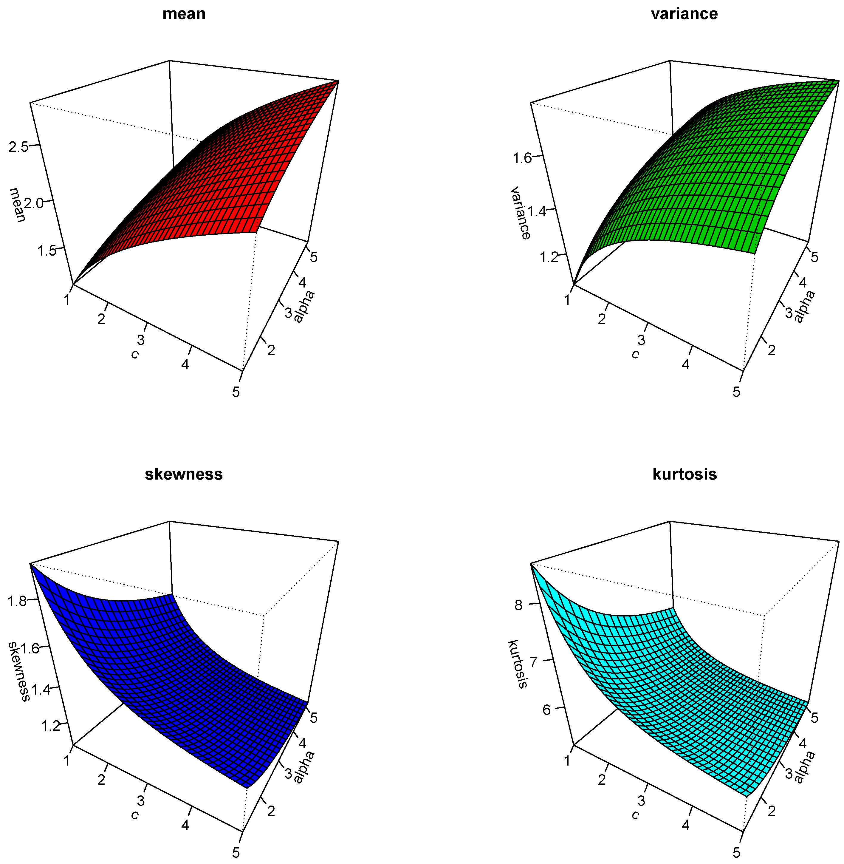
The plots of the mean, variance, skewness, and kurtosis of the APExE model for various parametric values of and c are displayed in Figure 3.
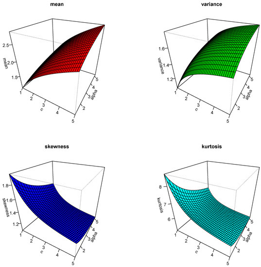
Figure 3.
Plots of the mean, variance, skewness, and kurtosis of the APExE model with .
The moment generating function of the APExE distribution takes the form
The characteristic function of the APExE distribution follows from the above equation by replacing t with .
3.3. Moments of Residual Life
Let be the SF of the APExE distribution, then its moment of residual life is given by
The mean residual life function of the APExE distribution is obtained by setting in the previous equation and then by setting , we have the mean of the APExE distribution.
3.4. Entropies
The entropy of a random variable X is a measure of variation of the uncertainty, and it has some applications in several applied areas such as statistics to test hypotheses in parametric models (see Morales et al. [22]), and information theory, engineering and physics for describing nonlinear chaotic or dynamical systems (see Kurths et al. [23]). Furthermore, Song [24] developed a log-likelihood-based distribution measure using the Rényi information which exists for all distributions and allows for meaningful comparisons between distributions than the traditional kurtosis measure. Song’s measure can be used in exploring density shapes especially for heavy-tailed distributions, while the kurtosis measure does not exist for many of these distributions.
In this section, we derive the continuous Rényi, Tsallis, and Shannon entropies of the APExE distribution. The Rényi, , and Tsallis, entropies of order r, where of the APExE distribution are given, respectively, by
and
The Rényi entropy reduces to Shannon entropy, , as r approaches to 1. The Shannon entropy of APExE distribution takes the form
where and is the Euler Mascheroni constant.
Table 1 reports some numerical values for the Rényi, Tsallis, and Shannon entropies of the APExE distribution.

Table 1.
Numerical values of Rényi, Tsallis, and Shannon entropies for the APExE distribution.
3.5. Inequality Curves
The most used and known important curves among inequality curves are Lorenz and Bonferroni that have useful applications in some applied areas including economics to study income and poverty, demography, reliability, medicine, and insurance.
The Lorenz and Bonferroni curves are defined for the APExE distribution as follows:
respectively, where is the QF of the APExE distribution.
3.6. Order Statistics
The PDF and CDF of the order statistic for the APExE distribution are
where is a hyper geometric function.
By setting , we have the PDF and CDF of minimum order statistics . The limit distribution for reduces to (see Theorem in Galambos [25])
By setting , we have the PDF and CDF of maximum order statistics . The limit distribution for takes the form (see Theorem in Galambos [25])
where .
4. Actuarial Measures
Probability distributions present a description of risk exposure. The level of risk exposure can be described by “key risk indicators” (numbers) that usually are functions of the model. Actuaries and risk managers often use such key risk indicators to determine the degree to which their companies are subject to particular aspects of risk, which arise from changes in underlying variables such as prices of equity, interest rates, or exchange rates.
In this section, we discuss the theoretical and computational aspects of some important risk measures including VaR, TVaR, TV, and TVP for the APExE distribution, which play a crucial role in portfolio optimization under uncertainty.
4.1. VaR Measure
The VaR is also known as the quantile risk measure or quantile premium principle, and it is specified with a given degree of confidence say q (typically , or ). Furthermore, VaR is a quantile of the distribution of aggregate losses. Risk managers are often interested in “the chance of an adverse outcome” that can be expressed through the VaR at a particular probability level. The VaR can be used to evaluate exposure to risk, and hence it is used to determine the amount of capital required to withstand such adverse outcomes. Investors, regulators, and rating agencies are particularly interested in the company’s ability to withstand such events. The VaR of a random variable X is the quantile of its CDF, denoted by , and it is defined by (see Artzner [26]).
If X has the PDF (2), then its VaR can be derived as
4.2. TVaR Measure
Another important measure is the TVaR that has been given several names including conditional tail expectation, conditional-value at-risk, and expected shortfall. The TVaR is used to quantify the expected value of the loss given that an event outside a given probability level has occurred. The TVaR is defined by
The TVaR of the APExE distribution is defined by
where .
4.3. TV Measure
Landsman [27] introduced the TV risk that is defined by the variance of the loss distribution beyond some critical value. The TV is one of the most important risk measures which pay attention to the tail variance beyond the VaR. The TV of the APExE distribution can be defined as
where
where , B and C are generalized hyper geometric functions given by and . Using Equations (6)–(8), we get the TV of APExE distribution.
4.4. TVP Measure
4.5. Numerical Simulations for Risk Measures
In this sub-section, we present some numerical results for the VaR, TVaR, TV, and TVP measures of the APExE, APE, ExE, and E distributions for different parametric values. The results are obtained through the following two steps:
- Random sample of size is generated from the APExE, APE, ExE and E distributions, and parameters have been estimated via the maximum likelihood method.
- 1000 repetitions are made to calculate the VaR, TVaR, TV, and TVP of the four distributions.
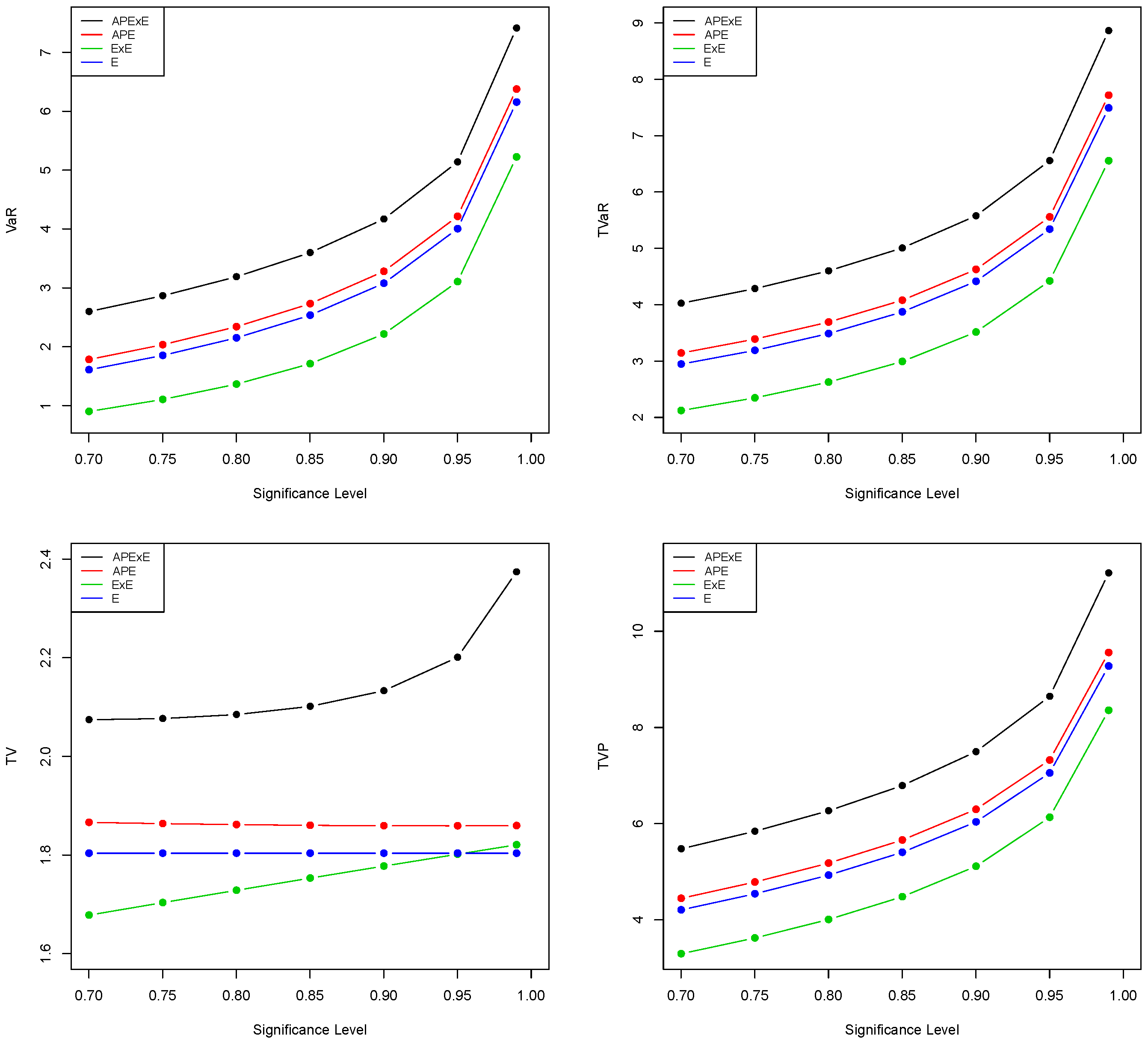
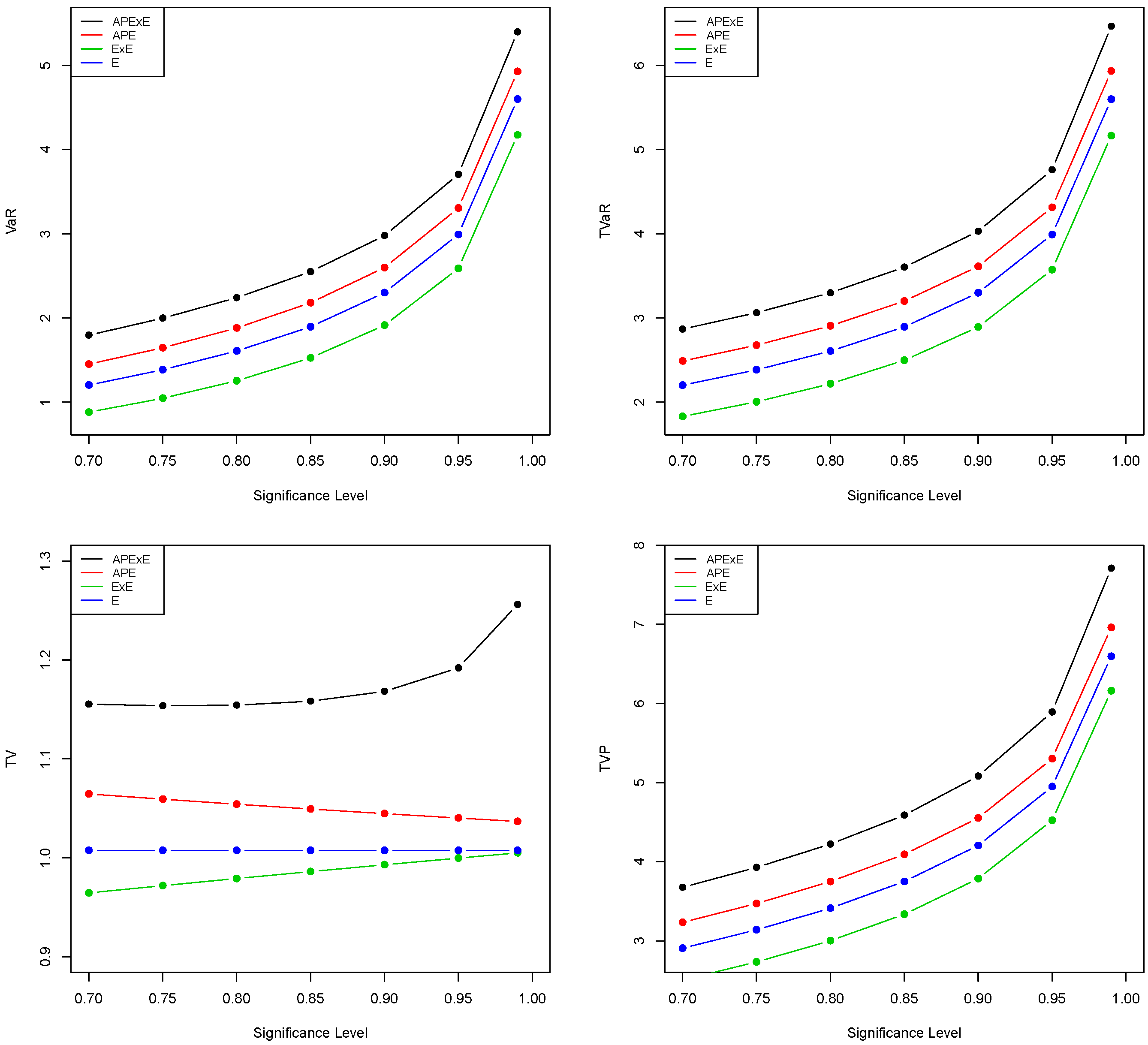
Simulation results of the VaR, TVaR, TV, and TVP for the APExE, APE, ExE, and E distributions are provided in Table 2 and Table 3. Furthermore, the results in these tables are depicted graphically in Figure 4 and Figure 5.

Table 2.
Simulation results for the VaR, TVaR, TV, and TVP of the APExE, APE, ExE, and E distributions.

Table 3.
Simulation results for the VaR, TVaR, TV, and TVP of the APExE, APE, ExE, and E distributions.
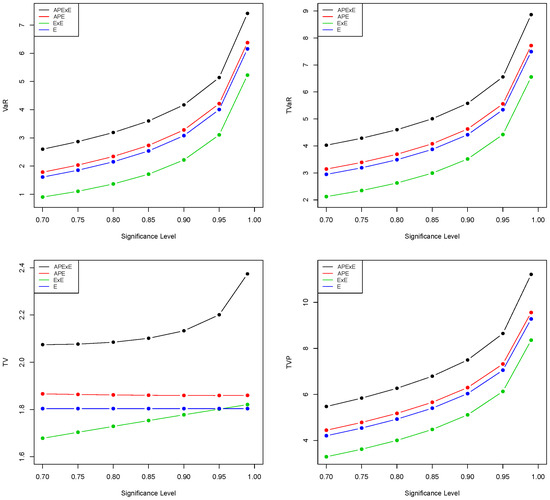
Figure 4.
Plots of the VaR, TVaR, TV, and TVP using the values in Table 2.
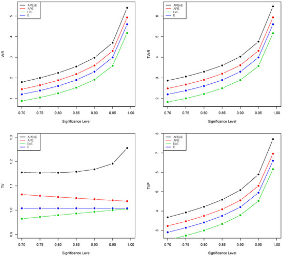
Figure 5.
Plots of the VaR, TVaR, TV, and TVP using the values in Table 3.
The model with higher values of VaR, TVaR, TV, and TVP measures is said to have a heavier tail than other competing models. The results in Table 2 and Table 3, and the plots in Figure 4 and Figure 5 show that the proposed APExE model has higher values of the four risk measures than the APE, ExE, and E distributions. Hence, the APExE model has a heavier tail than other distributions and can be utilized accurately to model heavy-tailed insurance data.
5. Methods of Estimation
In this section, we discuss the estimation of the APExE parameters by different methods of estimation including the MLE, OLSE, WLSE, ADE, CVME, and PE. Parameter estimation using different classical estimators have been discussed by many researchers. For example, the alpha logarithmic transformed Weibull distribution [28], quasi xgamma-geometric distribution [29], Weibull Marshall–Olkin Lindley distribution [30], and APE distribution [31], among others.
5.1. Maximum Likelihood Estimation
Let be a random sample of size n from the PDF (2), then the log-likelihood function reduces to
By differentiating Equation (10) with respect to , a and c, respectively, and equating to zero, we have
Solving the previous equations, we obtain estimators of the APExE parameters by the MLE.
5.2. Ordinary Least-Squares and Weighted Least-Squares Estimators
Let be the order statistics of a random sample of size n from the APExE distribution. Hence, we have the OLSE of the APExE parameters by minimizing the following equation:
The OLSE of the APExE parameters can also be obtained by solving the following nonlinear equations:
where
The WLSE of the APExE parameters can be calculated by minimizing the following equation:
Furthermore, the WLSE of the APExE parameters follow by solving the following nonlinear equations:
where were defined in (11), (12), and (13), respectively.
5.3. Anderson–Darling Estimation
The ADE of the APExE parameters are obtained by minimizing the following equation:
The ADE can also be calculated by solving the following nonlinear equations:
where were defined in (11), (12), and (13), respectively.
5.4. Cramér–von Mises Estimation
The CVME of APExE parameters are obtained by minimizing the following equation:
or by solving the following nonlinear equations
where were defined in (11), (12), and (13), respectively.
5.5. Percentile Estimation
Let be an estimate of , then the PE of the APExE parameters are obtained by minimizing the following equation:
or by solving the following nonlinear equations:
where
6. Simulation Results
In this section, we explore the performance of the aforementioned estimation methods in estimating the APExE parameters using simulation results. We consider various sample sizes, , and various parametric values, , and . We generate random samples from the APExE distribution via Equation (6). We determine the average values of the estimates ( AEs) along with their corresponding average absolute biases (ABs), average mean square error (MSEs), and average mean relative estimates (MREs) for all sample sizes and parameter combinations using the R software©.
The ABs, MSEs, and MREs can be calculated by the following respective equations:
where .
Table A1, Table A2, Table A3, Table A4, Table A5, Table A6, Table A7 and Table A8 report the simulation results including AEs, ABs, MSEs, and MREs of the APExE parameters using the six estimation approaches. These tables are given in Appendix A. One can note that the estimates of the APExE parameters obtained from all six estimation methods are entirely good, that is, these estimates are quite reliable and very close to the true values, showing small biases, MSEs and MREs in all parameter combinations. All six estimators show the consistency property, where the MSEs, ABs, and MREs decrease as sample size increases, for all parameter combinations. We conclude that the MLE, OLSE, WLSE, ADE, CVME, and PE methods perform very well in estimating the APExE parameters.
7. Modeling Insurance Data
In this section, we consider a heavy-tailed real data set from the insurance field to illustrate the usefulness of the APExE distribution. This data set represents monthly metrics on unemployment insurance from July 2008 to April 2013 including 58 observations, and it is reported by the Department of Labor, Licensing and Regulation, State of Maryland, USA. The data consist of 21 variables and we particularly analyze the variable number 12. The data are available at: https://catalog.data.gov/dataset/unemployment-insurance-data-july-2008-to-april-2013. We compare the goodness-of-fit results and some discrimination measures of the proposed distribution with some other well-known competing distributions, including the APE [20], ExE [21], beta exponential (BE) [32], E, extended odd Weibull exponential (EOWE) [33], exponentiated Weibull (ExW) [34], Weibull (W), transmuted generalized exponential (TGE) [35], Marshall–Olkin exponential (MOE) [36], generalized transmuted exponential (GTE) [37], transmuted exponentiated generalized exponential (TExGE) [38], complementary geometric transmuted exponential (CGTE) [39], gamma (G), Harris extended exponential (HEE) [40], and transmuted exponential (TE) [41] distributions.
The competing models can be compared using some discrimination measures such as Akaike information (AKI), consistent Akaike information (CAKI), Bayesian information (BAI), and Hannan–Quinn information (HAQUI) criteria. Further discrimination measures including Anderson Darling (ANDA), Cramér–von Mises (CRVMI), and Kolmogorov–Smirnov (KOSM) with its p-value.
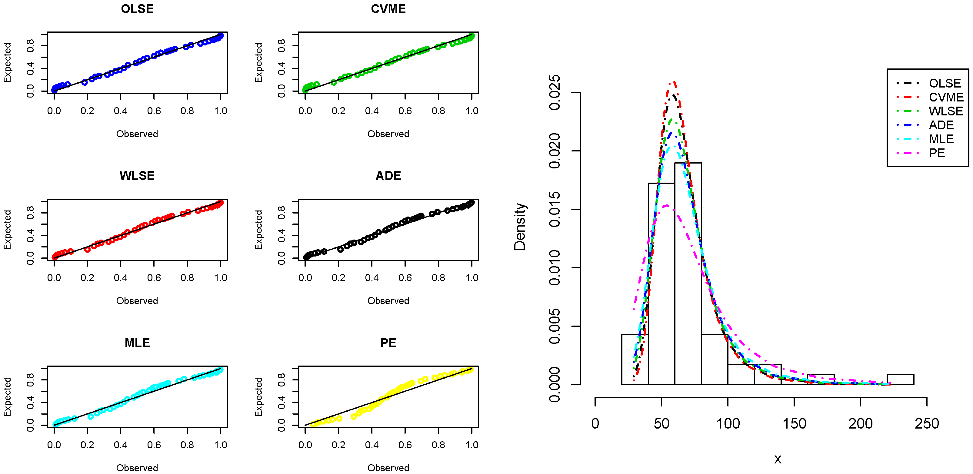
The MLEs and the analytical measures are computed using the R software©. Table 4 gives the MLEs and their standard errors. The analytical measures are provided in Table 5. The results in Table 5 indicate that the APExE provides better fits than other competing models and could be chosen as an adequate model to analyze the studied heavy-tailed insurance data. The fitted PDF, CDF, SF, and probability-probability (P–P) plots of the APExE model are depicted in Figure 6. Furthermore, we use the six estimation approaches discussed before in Section 5 to estimate the APExE parameters. Table 6 reports the estimates of the APExE parameters using these approaches and the numerical values of goodness-of-fit for insurance data. Based on the values of KOSM and p-values listed in Table 6, we conclude that the performance ordering of six estimators, from best to worst, for insurance data are OLSE, CVME, WLSE, ADE, MLE, and PE. The P–P plots and histogram of insurance data with the fitted APExE density for various estimation methods are shown in Figure 7 that supports the results in Table 6.

Table 4.
Estimated parameters with their standard errors of the APExE model and other fitted models.

Table 5.
Discrimination measures of the APExE model and other competing models.
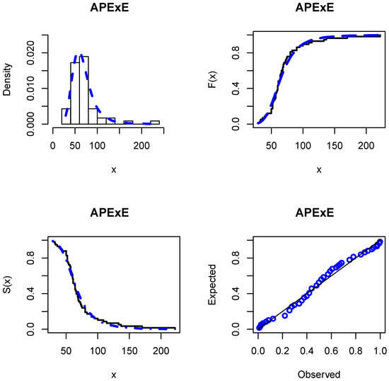
Figure 6.
The fitted APExE PDF, CDF, SF, and P–P plots for insurance data.

Table 6.
The estimates of the APExE parameters along with goodness-of-fit measures for insurance data.
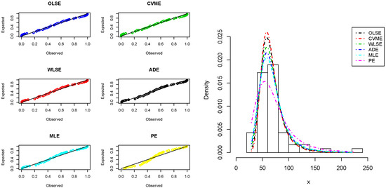
Figure 7.
The P–P plots and histogram of insurance data with the fitted APExE density for estimation methods.
8. Conclusions
In this paper, we propose a new heavy-tailed distribution to model heavy-tailed insurance data, called alpha power exponentiated exponential (APExE) distribution that extends the exponential (E), exponentiated exponential (ExE), and alpha power exponential (APE) distributions. Its associated hazard rate function can be bathtub, unimodal, decreasing, decreasing-constant, increasing, and reversed-J shaped. Some of its statistical properties are derived. The risk measures such as value at risk, tail value at risk, tail variance, and tail variance premium are derived for the APExE distribution along with a conducted simulation study for these actuarial measures, proving that the APExE distribution has a heavier tail than the APE, ExE, and E distributions. Its unknown parameters are estimated by six frequentist estimation approaches. The practical applicability of the APExE distribution has been illustrated by an insurance real-life data, proving its superiority over fifteen competing models.
The research in this article can be extended in some ways. For example, the APExE distribution can be utilized for analyzing and modeling data in other fields such as reliability engineering, medicine, economics, survival analyses, and life testing.
Bayesian estimation of the APExE parameters based on complete and several types of censored samples under different types of loss functions could be discussed. Furthermore, a bivariate extension of the APExE distribution may also be studied.
Author Contributions
A.Z.A., A.M.G. and N.A.I. contributed equally to this work. All authors have read and agreed to the published version of the manuscript.
Funding
This research received no external funding.
Acknowledgments
The authors would like to thank the Editorial Board, and two referees for their constructive remarks and suggestions which greatly improved the final version of this manuscript.
Conflicts of Interest
The authors declare no conflicts of interest.
Abbreviations
| CDF | Cumulative distribution function |
| Probability density function | |
| SF | Survival function |
| QF | Quantile function |
| HRF | Hazard rate function |
| VaR | Value at risk |
| TVar | Tail value at risk |
| TV | Tail variance |
| TVP | Tail variance premium |
| MLE | Maximum likelihood estimators |
| OLSE | Ordinary least-squares estimators |
| WLSE | Weighted-least-squares estimators |
| ADE | Anderson–Darling estimators |
| CVME | Cramér–von Mises estimators |
| PE | Percentile estimators |
| AEs | Average values of the estimates |
| ABs | Average absolute biases |
| MSEs | Average mean square error |
| MREs | Average mean relative estimates |
| AKI | Akaike information |
| CAKI | consistent Akaike information |
| BAI | Bayesian information |
| HAQUI | Hannan–Quinn information |
| ANDA | Anderson Darling |
| CRVMI | Cramér–von Mises |
| KOSM | Kolmogorov–Smirnov |
| P–P | probability-probability |
| APExE | Alpha power exponentiated exponential |
| ExE | Exponentiated exponential |
| E | exponential |
| APE | Alpha power exponential |
| BE | Beta exponential |
| EOWE | Extended odd Weibull exponential |
| ExW | Exponentiated Weibull |
| W | Weibull |
| TGE | Transmuted generalized exponential |
| MOE | Marshall–Olkin exponential |
| GTE | Generalized transmuted exponential |
| TExGE | Transmuted exponentiated generalized exponential |
| CGTE | Complementary geometric transmuted exponential |
| G | Gamma |
| HEE | Harris extended exponential |
| TE | Transmuted exponential |
Appendix A

Table A1.
The AEs, ABs, MSEs, and MREs for .
Table A1.
The AEs, ABs, MSEs, and MREs for .
| AEs | ABs | MSEs | MREs | ||||||||||
|---|---|---|---|---|---|---|---|---|---|---|---|---|---|
| Method | |||||||||||||
| MLE | 20 | 0.49429 | 0.51330 | 0.51074 | 0.09209 | 0.07908 | 0.06605 | 0.00895 | 0.00723 | 0.00554 | 0.18418 | 0.15816 | 0.13209 |
| 50 | 0.50291 | 0.51300 | 0.51255 | 0.08907 | 0.06948 | 0.05312 | 0.00855 | 0.00602 | 0.00391 | 0.17815 | 0.13897 | 0.10624 | |
| 100 | 0.50643 | 0.50955 | 0.50638 | 0.08728 | 0.06027 | 0.04149 | 0.00830 | 0.00482 | 0.00259 | 0.17455 | 0.12054 | 0.08298 | |
| 200 | 0.50175 | 0.50658 | 0.50543 | 0.08667 | 0.05194 | 0.03405 | 0.00823 | 0.00374 | 0.00178 | 0.17335 | 0.10388 | 0.06809 | |
| ADE | 20 | 0.50232 | 0.49713 | 0.50131 | 0.04771 | 0.04409 | 0.04123 | 0.00235 | 0.00211 | 0.00191 | 0.09542 | 0.08819 | 0.08246 |
| 50 | 0.50331 | 0.49744 | 0.50121 | 0.04631 | 0.04161 | 0.03597 | 0.00226 | 0.00195 | 0.00157 | 0.09262 | 0.08322 | 0.07194 | |
| 100 | 0.49648 | 0.50209 | 0.50032 | 0.04561 | 0.03896 | 0.03088 | 0.00221 | 0.00177 | 0.00125 | 0.09122 | 0.07792 | 0.06175 | |
| 200 | 0.49756 | 0.50190 | 0.50126 | 0.04426 | 0.03583 | 0.02618 | 0.00212 | 0.00155 | 0.00095 | 0.08852 | 0.07167 | 0.05236 | |
| CVME | 20 | 0.44678 | 0.48931 | 0.52387 | 0.14734 | 0.08400 | 0.07143 | 0.02989 | 0.00785 | 0.00627 | 0.29468 | 0.16800 | 0.14285 |
| 50 | 0.43848 | 0.48734 | 0.52188 | 0.14614 | 0.07719 | 0.06257 | 0.02924 | 0.00696 | 0.00510 | 0.29228 | 0.15437 | 0.12513 | |
| 100 | 0.44831 | 0.48581 | 0.51659 | 0.13633 | 0.07128 | 0.05391 | 0.02558 | 0.00625 | 0.00400 | 0.27266 | 0.14255 | 0.10782 | |
| 200 | 0.45154 | 0.48000 | 0.51335 | 0.13280 | 0.06533 | 0.04154 | 0.02414 | 0.00541 | 0.00258 | 0.26561 | 0.13065 | 0.08309 | |
| OLSE | 20 | 0.50862 | 0.48615 | 0.49541 | 0.09172 | 0.08181 | 0.06842 | 0.00887 | 0.00759 | 0.00581 | 0.18344 | 0.16361 | 0.13683 |
| 50 | 0.50814 | 0.48762 | 0.49785 | 0.08968 | 0.07586 | 0.05534 | 0.00862 | 0.00674 | 0.00418 | 0.17936 | 0.15173 | 0.11067 | |
| 100 | 0.50062 | 0.49167 | 0.49679 | 0.08878 | 0.06592 | 0.04527 | 0.00850 | 0.00552 | 0.00294 | 0.17755 | 0.13184 | 0.09054 | |
| 200 | 0.50256 | 0.49153 | 0.49772 | 0.08858 | 0.05547 | 0.03584 | 0.00848 | 0.00417 | 0.00197 | 0.17716 | 0.11094 | 0.07169 | |
| WLSE | 20 | 0.50335 | 0.48766 | 0.49226 | 0.09088 | 0.08232 | 0.06513 | 0.00879 | 0.00766 | 0.00547 | 0.18177 | 0.16464 | 0.13025 |
| 50 | 0.50023 | 0.49563 | 0.49867 | 0.08936 | 0.07407 | 0.05241 | 0.00859 | 0.00655 | 0.00382 | 0.17871 | 0.14814 | 0.10481 | |
| 100 | 0.49677 | 0.49706 | 0.50227 | 0.08852 | 0.06238 | 0.04387 | 0.00846 | 0.00505 | 0.00281 | 0.17705 | 0.12476 | 0.08773 | |
| 200 | 0.49767 | 0.50182 | 0.50412 | 0.08813 | 0.05208 | 0.03267 | 0.00841 | 0.00376 | 0.00165 | 0.17626 | 0.10415 | 0.06535 | |
| PE | 20 | 0.52555 | 0.47740 | 0.51429 | 0.09335 | 0.08291 | 0.07667 | 0.18670 | 0.16581 | 0.15334 | 0.18670 | 0.16581 | 0.15334 |
| 50 | 0.51727 | 0.46863 | 0.49572 | 0.09196 | 0.07780 | 0.06644 | 0.18392 | 0.15561 | 0.13288 | 0.18392 | 0.15561 | 0.13288 | |
| 100 | 0.50209 | 0.47350 | 0.48650 | 0.09026 | 0.07242 | 0.06021 | 0.18053 | 0.14483 | 0.12043 | 0.18053 | 0.14483 | 0.12043 | |
| 200 | 0.49351 | 0.47594 | 0.48729 | 0.08957 | 0.06429 | 0.05581 | 0.17914 | 0.12857 | 0.11161 | 0.17914 | 0.12857 | 0.11161 | |

Table A2.
The AEs, ABs, MSEs, and MREs for .
Table A2.
The AEs, ABs, MSEs, and MREs for .
| AEs | ABs | MSEs | MREs | ||||||||||
|---|---|---|---|---|---|---|---|---|---|---|---|---|---|
| Method | |||||||||||||
| MLE | 20 | 1.99030 | 0.51376 | 0.51136 | 0.19184 | 0.07348 | 0.07082 | 0.03787 | 0.00655 | 0.00613 | 0.09592 | 0.14696 | 0.14163 |
| 50 | 1.99100 | 0.50721 | 0.51217 | 0.19077 | 0.06323 | 0.05859 | 0.03767 | 0.00519 | 0.00458 | 0.09538 | 0.12645 | 0.11718 | |
| 100 | 1.99119 | 0.50688 | 0.51000 | 0.18885 | 0.05173 | 0.04920 | 0.03720 | 0.00373 | 0.00344 | 0.09442 | 0.10345 | 0.09840 | |
| 200 | 1.99023 | 0.50758 | 0.50585 | 0.18696 | 0.04040 | 0.03619 | 0.03669 | 0.00248 | 0.00202 | 0.09348 | 0.08079 | 0.07238 | |
| ADE | 20 | 1.99942 | 0.49763 | 0.49587 | 0.19195 | 0.07481 | 0.06944 | 0.03781 | 0.00668 | 0.00603 | 0.09597 | 0.14962 | 0.13888 |
| 50 | 2.00634 | 0.50083 | 0.50082 | 0.18989 | 0.06477 | 0.05838 | 0.03738 | 0.00535 | 0.00458 | 0.09495 | 0.12954 | 0.11676 | |
| 100 | 1.99476 | 0.50006 | 0.50195 | 0.18923 | 0.05279 | 0.04969 | 0.03710 | 0.00391 | 0.00348 | 0.09461 | 0.10558 | 0.09939 | |
| 200 | 2.00669 | 0.50318 | 0.50208 | 0.18745 | 0.04215 | 0.03882 | 0.03664 | 0.00265 | 0.00228 | 0.09373 | 0.08430 | 0.07764 | |
| CVME | 20 | 2.03250 | 0.51031 | 0.50510 | 0.32277 | 0.07458 | 0.07195 | 0.11214 | 0.00666 | 0.00627 | 0.16138 | 0.14915 | 0.14390 |
| 50 | 2.04455 | 0.50869 | 0.50601 | 0.32238 | 0.06709 | 0.06177 | 0.11189 | 0.00565 | 0.00499 | 0.16119 | 0.13418 | 0.12355 | |
| 100 | 2.03861 | 0.50413 | 0.50273 | 0.32058 | 0.05783 | 0.05006 | 0.11092 | 0.00443 | 0.00359 | 0.16029 | 0.11566 | 0.10012 | |
| 200 | 2.03448 | 0.50510 | 0.50315 | 0.31826 | 0.04682 | 0.04269 | 0.10969 | 0.00314 | 0.00267 | 0.15913 | 0.09364 | 0.08539 | |
| OLSE | 20 | 2.03997 | 0.48375 | 0.49568 | 0.44086 | 0.07665 | 0.07316 | 0.21238 | 0.00692 | 0.00647 | 0.22043 | 0.15331 | 0.14632 |
| 50 | 2.02901 | 0.49152 | 0.49704 | 0.43799 | 0.06783 | 0.06209 | 0.20881 | 0.00577 | 0.00506 | 0.21899 | 0.13566 | 0.12419 | |
| 100 | 2.01371 | 0.49639 | 0.50005 | 0.43696 | 0.05853 | 0.05481 | 0.20852 | 0.00459 | 0.00411 | 0.21848 | 0.11706 | 0.10961 | |
| 200 | 2.01453 | 0.49809 | 0.50472 | 0.43660 | 0.04640 | 0.04498 | 0.20791 | 0.00314 | 0.00295 | 0.21830 | 0.09280 | 0.08996 | |
| WLSE | 20 | 2.01427 | 0.49289 | 0.49113 | 0.36843 | 0.07652 | 0.07104 | 0.14320 | 0.00688 | 0.00621 | 0.18421 | 0.15304 | 0.14209 |
| 50 | 1.99966 | 0.49676 | 0.49939 | 0.36484 | 0.06656 | 0.05919 | 0.14084 | 0.00558 | 0.00467 | 0.18242 | 0.13312 | 0.11839 | |
| 100 | 2.03515 | 0.49557 | 0.50172 | 0.35806 | 0.05540 | 0.04953 | 0.13756 | 0.00420 | 0.00350 | 0.17903 | 0.11079 | 0.09906 | |
| 200 | 2.01349 | 0.50073 | 0.50401 | 0.35687 | 0.04338 | 0.04212 | 0.13694 | 0.00277 | 0.00261 | 0.17843 | 0.08675 | 0.08424 | |
| PE | 20 | 2.12964 | 0.46124 | 0.47823 | 0.30129 | 0.12978 | 0.12389 | 0.10217 | 0.02141 | 0.01994 | 0.15065 | 0.25955 | 0.24779 |
| 50 | 2.07355 | 0.46240 | 0.47181 | 0.28488 | 0.10534 | 0.11068 | 0.09188 | 0.01514 | 0.01672 | 0.14244 | 0.21068 | 0.22137 | |
| 100 | 2.03807 | 0.47166 | 0.47057 | 0.27639 | 0.08607 | 0.08974 | 0.08608 | 0.01075 | 0.01158 | 0.13870 | 0.17213 | 0.17947 | |
| 200 | 2.04661 | 0.48058 | 0.47571 | 0.27303 | 0.06186 | 0.06792 | 0.08588 | 0.00584 | 0.00706 | 0.13601 | 0.12371 | 0.13583 | |

Table A3.
The AEs, ABs, MSEs, and MREs for .
Table A3.
The AEs, ABs, MSEs, and MREs for .
| AEs | ABs | MSEs | MREs | ||||||||||
|---|---|---|---|---|---|---|---|---|---|---|---|---|---|
| Method | |||||||||||||
| MLE | 20 | 1.95092 | 1.47863 | 0.50578 | 0.40619 | 0.12256 | 0.07696 | 0.17873 | 0.01812 | 0.00783 | 0.20309 | 0.08171 | 0.15392 |
| 50 | 1.91835 | 1.48625 | 0.50869 | 0.40320 | 0.11155 | 0.06099 | 0.17724 | 0.01561 | 0.00511 | 0.20160 | 0.07437 | 0.12198 | |
| 100 | 1.88769 | 1.48459 | 0.51262 | 0.40008 | 0.10198 | 0.04925 | 0.17619 | 0.01356 | 0.00354 | 0.20004 | 0.06799 | 0.09850 | |
| 200 | 1.91756 | 1.48379 | 0.51005 | 0.38549 | 0.09322 | 0.04186 | 0.16672 | 0.01146 | 0.00261 | 0.19275 | 0.06215 | 0.08373 | |
| ADE | 20 | 2.00856 | 1.49588 | 0.51393 | 0.47681 | 0.09381 | 0.10027 | 0.23439 | 0.00916 | 0.01578 | 0.23841 | 0.06254 | 0.20054 |
| 50 | 1.98429 | 1.49783 | 0.51354 | 0.46765 | 0.08704 | 0.06865 | 0.22837 | 0.00828 | 0.00754 | 0.23382 | 0.05803 | 0.13731 | |
| 100 | 2.00514 | 1.49510 | 0.50690 | 0.44871 | 0.08462 | 0.05472 | 0.21522 | 0.00796 | 0.00468 | 0.22436 | 0.05641 | 0.10944 | |
| 200 | 2.02087 | 1.49116 | 0.50548 | 0.42898 | 0.07587 | 0.04227 | 0.20225 | 0.00681 | 0.00279 | 0.21449 | 0.05058 | 0.08454 | |
| CVME | 20 | 1.93732 | 1.51731 | 0.53416 | 0.46717 | 0.09339 | 0.10712 | 0.22935 | 0.00912 | 0.01808 | 0.23359 | 0.06226 | 0.21425 |
| 50 | 1.97703 | 1.50451 | 0.51809 | 0.46599 | 0.08872 | 0.07371 | 0.22814 | 0.00853 | 0.00911 | 0.23299 | 0.05915 | 0.14742 | |
| 100 | 1.97302 | 1.50208 | 0.51472 | 0.45597 | 0.08701 | 0.05791 | 0.22088 | 0.00825 | 0.00551 | 0.22799 | 0.05801 | 0.11582 | |
| 200 | 1.98525 | 1.50327 | 0.51014 | 0.43489 | 0.07891 | 0.04666 | 0.20753 | 0.00721 | 0.00343 | 0.21744 | 0.05261 | 0.09332 | |
| OLSE | 20 | 2.06512 | 1.48082 | 0.51193 | 0.47487 | 0.09266 | 0.10378 | 0.23473 | 0.00902 | 0.01685 | 0.23744 | 0.06177 | 0.20756 |
| 50 | 2.04507 | 1.48920 | 0.50330 | 0.47155 | 0.08888 | 0.07536 | 0.23163 | 0.00853 | 0.00934 | 0.23577 | 0.05925 | 0.15071 | |
| 100 | 2.01887 | 1.49448 | 0.50216 | .45121 | 0.08430 | 0.05381 | 0.21848 | 0.00792 | 0.00462 | 0.22560 | 0.05620 | 0.10761 | |
| 200 | 2.02143 | 1.49272 | 0.50187 | 0.43887 | 0.07957 | 0.04476 | 0.20909 | 0.00727 | 0.00313 | 0.21943 | 0.05305 | 0.08953 | |
| WLSE | 20 | 2.11441 | 1.49127 | 0.49304 | 0.37496 | 0.09275 | 0.06988 | 0.15622 | 0.00906 | 0.00605 | 0.18748 | 0.06183 | 0.13975 |
| 50 | 2.10743 | 1.49499 | 0.49564 | 0.36414 | 0.08797 | 0.05684 | 0.15084 | 0.00840 | 0.00433 | 0.18207 | 0.05864 | 0.11367 | |
| 100 | 2.08991 | 1.50291 | 0.49575 | 0.36317 | 0.08268 | 0.04622 | 0.14792 | 0.00768 | 0.00309 | 0.18159 | 0.05512 | 0.09244 | |
| 200 | 2.10289 | 1.50092 | 0.49829 | 0.35583 | 0.07770 | 0.03921 | 0.14608 | 0.00706 | 0.00229 | 0.17792 | 0.05180 | 0.07843 | |
| PE | 20 | 2.21283 | 1.47193 | 0.51166 | 0.40805 | 0.09383 | 0.07742 | 0.18164 | 0.00914 | 0.00702 | 0.20402 | 0.06255 | 0.15485 |
| 50 | 2.20788 | 1.46869 | 0.50735 | 0.40236 | 0.08975 | 0.06643 | 0.17841 | 0.00863 | 0.00562 | 0.20118 | 0.05984 | 0.13285 | |
| 100 | 2.17682 | 1.47167 | 0.49897 | 0.39531 | 0.08702 | 0.05316 | 0.17213 | 0.00829 | 0.00392 | 0.19766 | 0.05801 | 0.10633 | |
| 200 | 2.13365 | 1.47332 | 0.49006 | 0.38478 | 0.08416 | 0.04545 | 0.16350 | 0.00785 | 0.00296 | 0.19239 | 0.05611 | 0.09091 | |

Table A4.
The AEs, ABs, MSEs, and MREs for .
Table A4.
The AEs, ABs, MSEs, and MREs for .
| AEs | ABs | MSEs | MREs | ||||||||||
|---|---|---|---|---|---|---|---|---|---|---|---|---|---|
| Method | |||||||||||||
| MLE | 20 | 1.90575 | 1.48684 | 3.08247 | 0.41613 | 0.10653 | 0.39385 | 0.18518 | 0.01446 | 0.17911 | 0.20806 | 0.07102 | 0.13128 |
| 50 | 1.90493 | 1.48784 | 3.06355 | 0.40262 | 0.09259 | 0.34392 | 0.17748 | 0.01142 | 0.14746 | 0.20131 | 0.06173 | 0.11464 | |
| 100 | 1.91548 | 1.49199 | 3.05693 | 0.38741 | 0.08492 | 0.31594 | 0.16844 | 0.00994 | 0.12890 | 0.19370 | 0.05662 | 0.10531 | |
| 200 | 1.93326 | 1.49271 | 3.04026 | 0.38561 | 0.07056 | 0.26763 | 0.16605 | 0.00704 | 0.10052 | 0.19280 | 0.04704 | 0.08921 | |
| ADE | 20 | 1.89539 | 1.46164 | 2.94206 | 0.41643 | 0.11170 | 0.38176 | 0.18611 | 0.01602 | 0.17197 | 0.20821 | 0.07447 | 0.12725 |
| 50 | 1.91628 | 1.47359 | 2.99873 | 0.39949 | 0.10039 | 0.36059 | 0.17510 | 0.01318 | 0.15568 | 0.19975 | 0.06693 | 0.12020 | |
| 100 | 1.91697 | 1.48110 | 2.99628 | 0.38777 | 0.08968 | 0.31907 | 0.16843 | 0.01101 | 0.13048 | 0.19388 | 0.05979 | 0.10636 | |
| 200 | 1.90373 | 1.48471 | 3.02791 | 0.38224 | 0.07732 | 0.27984 | 0.16523 | 0.00841 | 0.10665 | 0.19112 | 0.05155 | 0.09328 | |
| CVME | 20 | 1.91625 | 1.47001 | 3.00302 | 0.40681 | 0.11092 | 0.39620 | 0.17987 | 0.01582 | 0.18053 | 0.20341 | 0.07395 | 0.13207 |
| 50 | 1.90316 | 1.47808 | 3.04251 | 0.39691 | 0.10233 | 0.36276 | 0.17391 | 0.01373 | 0.15978 | 0.19846 | 0.06822 | 0.12092 | |
| 100 | 1.90716 | 1.48511 | 3.04471 | 0.38571 | 0.09095 | 0.33434 | 0.16658 | 0.01130 | 0.14176 | 0.19285 | 0.06063 | 0.11145 | |
| 200 | 1.91176 | 1.48817 | 3.04623 | 0.38045 | 0.08156 | 0.29805 | 0.16331 | 0.00922 | 0.11812 | 0.19022 | 0.05437 | 0.09935 | |
| OLSE | 20 | 1.93345 | 1.49679 | 3.07456 | 0.43800 | 0.08428 | 0.27356 | 0.20861 | 0.00790 | 0.09833 | 0.21900 | 0.05619 | 0.09119 |
| 50 | 1.92097 | 1.49647 | 3.05617 | 0.41169 | 0.07800 | 0.25254 | 0.19175 | 0.00704 | 0.08694 | 0.20584 | 0.05200 | 0.08415 | |
| 100 | 1.89309 | 1.49499 | 3.07546 | 0.39370 | 0.07387 | 0.25216 | 0.18033 | 0.00654 | 0.08690 | 0.19685 | 0.04925 | 0.08409 | |
| 200 | 1.92904 | 1.49433 | 3.05546 | 0.38635 | 0.06789 | 0.23046 | 0.17403 | 0.00575 | 0.07405 | 0.19317 | 0.04526 | 0.07682 | |
| WLSE | 20 | 1.99071 | 1.47470 | 2.95573 | 0.04954 | 0.10447 | 0.18157 | 0.00247 | 0.01440 | 0.03510 | 0.02477 | 0.06964 | 0.06052 |
| 20 | 1.99049 | 1.48456 | 2.96394 | 0.04944 | 0.08428 | 0.17261 | 0.00246 | 0.00983 | 0.03273 | 0.02472 | 0.05619 | 0.05754 | |
| 100 | 1.99205 | 1.49169 | 2.97633 | 0.04925 | 0.07023 | 0.16445 | 0.00245 | 0.00701 | 0.03076 | 0.02463 | 0.04682 | 0.05482 | |
| 200 | 1.99681 | 1.50024 | 2.99031 | 0.04916 | 0.05478 | 0.15674 | 0.00244 | 0.00452 | 0.02857 | 0.02458 | 0.03652 | 0.05225 | |
| PE | 20 | 1.99682 | 1.43802 | 2.88990 | 0.04957 | 0.12478 | 0.38735 | 0.00247 | 0.01947 | 0.17476 | 0.02479 | 0.08319 | 0.12912 |
| 50 | 1.99214 | 1.44187 | 2.85397 | 0.04938 | 0.11444 | 0.35925 | 0.00246 | 0.01706 | 0.15601 | 0.02469 | 0.07630 | 0.11975 | |
| 100 | 1.98632 | 1.45081 | 2.84300 | 0.04927 | 0.09965 | 0.34272 | 0.00245 | 0.01343 | 0.14548 | 0.02464 | 0.06643 | 0.11424 | |
| 200 | 1.98246 | 1.45661 | 2.86540 | 0.04921 | 0.08777 | 0.31131 | 0.00245 | 0.01073 | 0.12629 | 0.02460 | 0.05851 | 0.10377 | |

Table A5.
The AEs, ABs, MSEs, and MREs for .
Table A5.
The AEs, ABs, MSEs, and MREs for .
| AEs | ABs | MSEs | MREs | ||||||||||
|---|---|---|---|---|---|---|---|---|---|---|---|---|---|
| Method | |||||||||||||
| MLE | 20 | 0.44893 | 1.47999 | 0.51836 | 0.13319 | 0.12530 | 0.07178 | 0.02105 | 0.01872 | 0.00677 | 0.26639 | 0.08354 | 0.14355 |
| 50 | 0.45794 | 1.47563 | 0.51667 | 0.12486 | 0.12045 | 0.05686 | 0.01885 | 0.01763 | 0.00446 | 0.24971 | 0.08030 | 0.11371 | |
| 100 | 0.45934 | 1.46441 | 0.51168 | 0.11909 | 0.12021 | 0.04455 | 0.01752 | 0.01785 | 0.00294 | 0.23817 | 0.08014 | 0.08909 | |
| 200 | 0.46604 | 1.46776 | 0.50855 | 0.11252 | 0.10795 | 0.03515 | 0.01581 | 0.01514 | 0.00195 | 0.22504 | 0.07197 | 0.07030 | |
| ADE | 20 | 0.47160 | 1.44672 | 0.50761 | 0.12836 | 0.13625 | 0.07003 | 0.01953 | 0.02199 | 0.00660 | 0.25672 | 0.09084 | 0.14006 |
| 50 | 0.45994 | 1.44124 | 0.51046 | 0.12349 | 0.13442 | 0.05475 | 0.01847 | 0.02172 | 0.00431 | 0.24699 | 0.08962 | 0.10951 | |
| 100 | 0.45391 | 1.44934 | 0.51429 | 0.12071 | 0.12459 | 0.04646 | 0.01806 | 0.01917 | 0.00317 | 0.24143 | 0.08306 | 0.09291 | |
| 200 | 0.46225 | 1.44600 | 0.50939 | 0.11033 | 0.11731 | 0.03735 | 0.01560 | 0.01771 | 0.00212 | 0.22067 | 0.07821 | 0.07469 | |
| CVME | 20 | 0.49987 | 1.50186 | 0.50531 | 0.04746 | 0.09380 | 0.06752 | 0.00234 | 0.00917 | 0.00571 | 0.09493 | 0.06253 | 0.13504 |
| 50 | 0.49791 | 1.50297 | 0.50347 | 0.04737 | 0.08949 | 0.05080 | 0.00233 | 0.00859 | 0.00366 | 0.09474 | 0.05966 | 0.10161 | |
| 100 | 0.49712 | 1.50287 | 0.50397 | 0.04649 | 0.08801 | 0.04002 | 0.00227 | 0.00843 | 0.00245 | 0.09298 | 0.05867 | 0.08004 | |
| 200 | 0.50254 | 1.49432 | 0.50172 | 0.04574 | 0.08278 | 0.02875 | 0.00222 | 0.00774 | 0.00131 | 0.09148 | 0.05518 | 0.05750 | |
| OLSE | 20 | 0.50660 | 1.48350 | 0.49639 | 0.04816 | 0.09448 | 0.06709 | 0.00237 | 0.00926 | 0.00566 | 0.09632 | 0.06298 | 0.13417 |
| 50 | 0.50422 | 1.48646 | 0.49435 | 0.04749 | 0.09052 | 0.05175 | 0.00233 | 0.00874 | 0.00377 | 0.09497 | 0.06034 | 0.10350 | |
| 100 | 0.50265 | 1.49215 | 0.49890 | 0.04713 | 0.08775 | 0.04013 | 0.00231 | 0.00838 | 0.00242 | 0.09426 | 0.05850 | 0.08025 | |
| 200 | 0.50096 | 1.49265 | 0.50177 | 0.04594 | 0.08330 | 0.02898 | 0.00223 | 0.00776 | 0.00133 | 0.09189 | 0.05554 | 0.05795 | |
| WLSE | 20 | 0.50113 | 1.49225 | 0.49513 | 0.04782 | 0.09373 | 0.06854 | 0.00236 | 0.00915 | 0.00579 | 0.09565 | 0.06249 | 0.13708 |
| 50 | 0.50101 | 1.49421 | 0.50093 | 0.04723 | 0.09024 | 0.05114 | 0.00232 | 0.00868 | 0.00364 | 0.09445 | 0.06016 | 0.10228 | |
| 100 | 0.50148 | 1.49185 | 0.50120 | 0.04644 | 0.08814 | 0.03809 | 0.00226 | 0.00841 | 0.00223 | 0.09287 | 0.05876 | 0.07618 | |
| 200 | 0.49816 | 1.49748 | 0.50185 | 0.04603 | 0.08102 | 0.02886 | 0.00224 | 0.00748 | 0.00130 | 0.09205 | 0.05402 | 0.05772 | |
| PE | 20 | 0.51263 | 1.47425 | 0.51912 | 0.04891 | 0.09520 | 0.07880 | 0.00243 | 0.00935 | 0.00721 | 0.09782 | 0.06347 | 0.15759 |
| 50 | 0.51506 | 1.47151 | 0.52122 | 0.04845 | 0.09249 | 0.06937 | 0.00240 | 0.00900 | 0.00595 | 0.09690 | 0.06166 | 0.13874 | |
| 100 | 0.51296 | 1.46755 | 0.51050 | 0.04784 | 0.08986 | 0.05750 | 0.00236 | 0.00867 | 0.00447 | 0.09569 | 0.05990 | 0.11500 | |
| 200 | 0.51032 | 1.47434 | 0.50326 | 0.04766 | 0.08812 | 0.04423 | 0.00235 | 0.00840 | 0.00285 | 0.09533 | 0.05875 | 0.08846 | |

Table A6.
The AEs, ABs, MSEs, and MREs for .
Table A6.
The AEs, ABs, MSEs, and MREs for .
| AEs | ABs | MSEs | MREs | ||||||||||
|---|---|---|---|---|---|---|---|---|---|---|---|---|---|
| Method | |||||||||||||
| MLE | 20 | 0.48970 | 1.47264 | 2.97345 | 0.09109 | 0.11684 | 0.21614 | 0.00882 | 0.02013 | 0.05247 | 0.18219 | 0.07789 | 0.07205 |
| 50 | 0.49660 | 1.48197 | 2.98771 | 0.09098 | 0.09904 | 0.19932 | 0.00880 | 0.01447 | 0.04639 | 0.18196 | 0.06603 | 0.06644 | |
| 100 | 0.49528 | 1.49105 | 2.98522 | 0.08872 | 0.08547 | 0.18765 | 0.00849 | 0.01032 | 0.04282 | 0.17744 | 0.05698 | 0.06255 | |
| 200 | 0.49668 | 1.49662 | 3.00523 | 0.08743 | 0.07363 | 0.16368 | 0.00835 | 0.00771 | 0.03374 | 0.17486 | 0.04909 | 0.05456 | |
| ADE | 20 | 0.44427 | 1.45604 | 2.99165 | 0.13571 | 0.11229 | 0.25374 | 0.02180 | 0.01640 | 0.07139 | 0.27143 | 0.07486 | 0.08458 |
| 50 | 0.43290 | 1.46031 | 2.98915 | 0.13431 | 0.10361 | 0.23943 | 0.02170 | 0.01439 | 0.06587 | 0.26861 | 0.06880 | 0.07981 | |
| 100 | 0.44713 | 1.44637 | 2.99080 | 0.12588 | 0.10224 | 0.22959 | 0.01954 | 0.01416 | 0.06133 | 0.25175 | 0.06843 | 0.07653 | |
| 200 | 0.45308 | 1.45530 | 2.99265 | 0.12436 | 0.09061 | 0.19993 | 0.01904 | 0.01166 | 0.05018 | 0.24872 | 0.06041 | 0.06664 | |
| CVME | 20 | 0.51399 | 1.53061 | 3.01520 | 0.09074 | 0.10916 | 0.09525 | 0.00879 | 0.01538 | 0.00937 | 0.18147 | 0.07277 | 0.03175 |
| 50 | 0.51267 | 1.52197 | 3.01816 | 0.08946 | 0.09118 | 0.09375 | 0.00859 | 0.01163 | 0.00917 | 0.17892 | 0.06079 | 0.03125 | |
| 100 | 0.51477 | 1.50753 | 3.00556 | 0.08894 | 0.07651 | 0.09123 | 0.00847 | 0.00836 | 0.00883 | 0.17788 | 0.05100 | 0.03041 | |
| 200 | 0.50357 | 1.50638 | 3.00538 | 0.08776 | 0.06793 | 0.08950 | 0.00838 | 0.00665 | 0.00861 | 0.17551 | 0.04528 | 0.02983 | |
| OLSE | 20 | 0.50027 | 1.48817 | 2.94953 | 0.04766 | 0.08339 | 0.13944 | 0.00235 | 0.00779 | 0.02263 | 0.09532 | 0.05559 | 0.04648 |
| 50 | 0.50134 | 1.48874 | 2.94830 | 0.04617 | 0.07580 | 0.13327 | 0.00225 | 0.00676 | 0.02127 | 0.09234 | 0.05053 | 0.04442 | |
| 100 | 0.50172 | 1.48537 | 2.94841 | 0.04561 | 0.06822 | 0.12900 | 0.00223 | 0.00581 | 0.02027 | 0.09221 | 0.04548 | 0.04300 | |
| 200 | 0.50267 | 1.48848 | 2.96272 | 0.04507 | 0.05864 | 0.12064 | 0.00221 | 0.00463 | 0.01797 | 0.09113 | 0.03909 | 0.04021 | |
| WLSE | 20 | 0.49794 | 1.49819 | 2.98235 | 0.04814 | 0.08016 | 0.17681 | 0.00237 | 0.00743 | 0.03373 | 0.09628 | 0.05344 | 0.05894 |
| 50 | 0.50058 | 1.49326 | 3.00066 | 0.04721 | 0.07442 | 0.16369 | 0.00231 | 0.00660 | 0.03033 | 0.09441 | 0.04961 | 0.05456 | |
| 100 | 0.49673 | 1.49743 | 2.99070 | 0.04575 | 0.06733 | 0.15784 | 0.00222 | 0.00571 | 0.02871 | 0.09159 | 0.04489 | 0.05261 | |
| 200 | 0.49916 | 1.49503 | 2.99735 | 0.04556 | 0.06103 | 0.14676 | 0.00221 | 0.00491 | 0.02605 | 0.09102 | 0.04069 | 0.04892 | |
| PE | 20 | 0.50975 | 1.47135 | 3.00965 | 0.04745 | 0.08714 | 0.17785 | 0.00233 | 0.00829 | 0.03403 | 0.09490 | 0.05810 | 0.05928 |
| 50 | 0.50683 | 1.47543 | 2.98678 | 0.04722 | 0.08359 | 0.16633 | 0.00232 | 0.00780 | 0.03101 | 0.09444 | 0.05573 | 0.05544 | |
| 100 | 0.50181 | 1.47720 | 2.97307 | 0.04520 | 0.07904 | 0.15933 | 0.00218 | 0.00721 | 0.02912 | 0.09040 | 0.05270 | 0.05311 | |
| 200 | 0.49846 | 1.47443 | 2.96308 | 0.04402 | 0.07222 | 0.14971 | 0.00210 | 0.00636 | 0.02674 | 0.08804 | 0.04815 | 0.04990 | |

Table A7.
The AEs, ABs, MSEs, and MREs for .
Table A7.
The AEs, ABs, MSEs, and MREs for .
| AEs | ABs | MSEs | MREs | ||||||||||
|---|---|---|---|---|---|---|---|---|---|---|---|---|---|
| Method | |||||||||||||
| MLE | 20 | 0.64736 | 0.50453 | 2.98921 | 0.39520 | 0.09017 | 0.23920 | 0.17490 | 0.01209 | 0.06795 | 0.79041 | 0.18034 | 0.07973 |
| 50 | 0.61230 | 0.49620 | 2.95488 | 0.37197 | 0.07935 | 0.23248 | 0.16095 | 0.00867 | 0.06666 | 0.74394 | 0.15870 | 0.07749 | |
| 100 | 0.61383 | 0.49630 | 2.95650 | 0.35090 | 0.07053 | 0.21340 | 0.14808 | 0.00710 | 0.05843 | 0.70181 | 0.14105 | 0.07113 | |
| 200 | 0.57303 | 0.49160 | 2.96619 | 0.31240 | 0.06276 | 0.18750 | 0.12419 | 0.00576 | 0.04678 | 0.62479 | 0.12551 | 0.06250 | |
| ADE | 20 | 0.59594 | 0.48656 | 2.91129 | 0.38417 | 0.09516 | 0.26195 | 0.16650 | 0.01324 | 0.08256 | 0.76834 | 0.19032 | 0.08732 |
| 50 | 0.57415 | 0.48272 | 2.91905 | 0.36896 | 0.08415 | 0.25176 | 0.15699 | 0.00945 | 0.07699 | 0.73791 | 0.16829 | 0.08392 | |
| 100 | 0.58554 | 0.48275 | 2.91575 | 0.36026 | 0.07695 | 0.22938 | 0.15197 | 0.00794 | 0.06743 | 0.72053 | 0.15391 | 0.07646 | |
| 200 | 0.57580 | 0.48474 | 2.92652 | 0.33971 | 0.07094 | 0.20520 | 0.13922 | 0.00683 | 0.05524 | 0.67942 | 0.14187 | 0.06840 | |
| CVME | 20 | 0.50455 | 0.49727 | 2.95329 | 0.04752 | 0.03779 | 0.23739 | 0.00234 | 0.00170 | 0.06951 | 0.09505 | 0.07558 | 0.07913 |
| 50 | 0.50676 | 0.49459 | 2.95007 | 0.04740 | 0.03280 | 0.22266 | 0.00233 | 0.00138 | 0.06257 | 0.09479 | 0.06560 | 0.07422 | |
| 100 | 0.50380 | 0.49706 | 2.96360 | 0.04717 | 0.02965 | 0.21293 | 0.00231 | 0.00116 | 0.05821 | 0.09435 | 0.05930 | 0.07098 | |
| 200 | 0.50391 | 0.49619 | 2.97183 | 0.04668 | 0.02602 | 0.19631 | 0.00228 | 0.00094 | 0.05004 | 0.09335 | 0.05204 | 0.06544 | |
| OLSE | 20 | 0.50087 | 0.49094 | 2.87601 | 0.04801 | 0.03837 | 0.33254 | 0.00236 | 0.00174 | 0.13163 | 0.09602 | 0.07674 | 0.11085 |
| 50 | 0.50395 | 0.49354 | 2.93578 | 0.04787 | 0.03399 | 0.27946 | 0.00235 | 0.00145 | 0.09894 | 0.09575 | 0.06798 | 0.09315 | |
| 100 | 0.50389 | 0.49207 | 2.93704 | 0.04733 | 0.03197 | 0.26648 | 0.00232 | 0.00131 | 0.09044 | 0.09467 | 0.06394 | 0.08883 | |
| 200 | 0.50689 | 0.49556 | 2.95854 | 0.04661 | 0.02792 | 0.23050 | 0.00227 | 0.00105 | 0.07058 | 0.09321 | 0.05584 | 0.07683 | |
| WLSE | 20 | 0.50019 | 0.49544 | 2.97812 | 0.04761 | 0.03932 | 0.30865 | 0.00235 | 0.00179 | 0.11154 | 0.09522 | 0.07864 | 0.10288 |
| 50 | 0.49742 | 0.49665 | 2.98502 | 0.04736 | 0.03483 | 0.28284 | 0.00232 | 0.00150 | 0.09798 | 0.09472 | 0.06966 | 0.09428 | |
| 100 | 0.49704 | 0.49945 | 3.00371 | 0.04693 | 0.03117 | 0.26000 | 0.00230 | 0.00126 | 0.08544 | 0.09387 | 0.06234 | 0.08667 | |
| 200 | 0.49687 | 0.49870 | 3.00274 | 0.04692 | 0.02749 | 0.22710 | 0.00229 | 0.00104 | 0.06920 | 0.09385 | 0.05499 | 0.07570 | |
| PE | 20 | 0.51243 | 0.48365 | 2.93035 | 0.04788 | 0.04018 | 0.31427 | 0.00236 | 0.00186 | 0.11887 | 0.09577 | 0.08036 | 0.10476 |
| 50 | 0.51014 | 0.48577 | 2.91254 | 0.04716 | 0.03853 | 0.28111 | 0.00231 | 0.00174 | 0.10079 | 0.09431 | 0.07706 | 0.09370 | |
| 100 | 0.50613 | 0.48596 | 2.88352 | 0.04650 | 0.03576 | 0.27995 | 0.00226 | 0.00156 | 0.10035 | 0.09299 | 0.07153 | 0.09332 | |
| 200 | 0.49612 | 0.48696 | 2.89119 | 0.04620 | 0.03201 | 0.26422 | 0.00225 | 0.00132 | 0.09045 | 0.09240 | 0.06403 | 0.08807 | |

Table A8.
The AEs, ABs, MSEs, and MREs for .
Table A8.
The AEs, ABs, MSEs, and MREs for .
| AEs | ABs | MSEs | MREs | ||||||||||
|---|---|---|---|---|---|---|---|---|---|---|---|---|---|
| Method | |||||||||||||
| MLE | 20 | 2.01611 | 0.50174 | 2.97926 | 0.28273 | 0.03736 | 0.23811 | 0.08320 | 0.00166 | 0.06825 | 0.14136 | 0.07472 | 0.07937 |
| 50 | 2.03662 | 0.49735 | 2.98232 | 0.27283 | 0.03179 | 0.22155 | 0.07937 | 0.00131 | 0.06067 | 0.13642 | 0.06359 | 0.07385 | |
| 100 | 2.02276 | 0.49908 | 2.99057 | 0.27276 | 0.02723 | 0.20989 | 0.07926 | 0.00102 | 0.05464 | 0.13638 | 0.05446 | 0.06996 | |
| 200 | 2.03926 | 0.50030 | 2.98488 | 0.27144 | 0.02266 | 0.19129 | 0.07873 | 0.00075 | 0.04804 | 0.13572 | 0.04533 | 0.06376 | |
| ADE | 20 | 1.96129 | 0.49123 | 2.92514 | 0.35253 | 0.03728 | 0.25122 | 0.13961 | 0.00165 | 0.07641 | .17626 | 0.07455 | 0.08374 |
| 50 | 1.97187 | 0.49524 | 2.94914 | 0.33427 | 0.03234 | 0.23479 | 0.12782 | 0.00134 | 0.06854 | 0.16714 | 0.06467 | 0.07826 | |
| 100 | 1.97514 | 0.49249 | 2.94603 | 0.32915 | 0.02901 | 0.22715 | 0.12567 | 0.00113 | 0.06389 | 0.16457 | 0.05803 | 0.07572 | |
| 200 | 1.99259 | 0.49515 | 2.96885 | 0.32491 | 0.02361 | 0.20108 | 0.12127 | 0.00082 | 0.05286 | 0.16245 | 0.04722 | 0.06703 | |
| CVME | 20 | 1.97750 | 0.49501 | 2.96586 | 0.34121 | 0.03715 | 0.24342 | 0.13258 | 0.00166 | 0.07096 | 0.17060 | 0.07429 | 0.08114 |
| 50 | 2.00867 | 0.49594 | 2.99050 | 0.33137 | 0.03216 | 0.22747 | 0.12440 | 0.00134 | 0.06290 | 0.16569 | 0.06433 | 0.07582 | |
| 100 | 2.00671 | 0.49525 | 2.95567 | 0.32929 | 0.02837 | 0.22696 | 0.12424 | 0.00110 | 0.06397 | 0.16464 | 0.05674 | 0.07565 | |
| 200 | 1.98458 | 0.49610 | 2.97665 | 0.32584 | 0.02559 | 0.20441 | 0.12150 | 0.00092 | 0.05363 | 0.16292 | 0.05119 | 0.06814 | |
| OLSE | 20 | 1.95478 | 0.49048 | 2.91470 | 0.34805 | 0.03802 | 0.26080 | 0.13781 | 0.00171 | 0.08143 | 0.17402 | 0.07604 | 0.08693 |
| 50 | 1.97065 | 0.49115 | 2.92102 | 0.33617 | 0.03335 | 0.24500 | 0.12852 | 0.00140 | 0.07430 | 0.16808 | 0.06669 | 0.08167 | |
| 100 | 1.98205 | 0.49310 | 2.94491 | 0.32891 | 0.03085 | 0.23563 | 0.12412 | 0.00123 | 0.06847 | 0.16445 | 0.06170 | 0.07854 | |
| 200 | 1.98150 | 0.49308 | 2.95659 | 0.32288 | 0.02632 | 0.21036 | 0.12049 | 0.00097 | 0.05661 | 0.16144 | 0.05264 | 0.07012 | |
| WLSE | 20 | 1.94604 | 0.49353 | 2.91373 | 0.35632 | 0.03728 | 0.25976 | 0.14211 | 0.00165 | 0.08039 | 0.17816 | 0.07456 | 0.08659 |
| 50 | 1.96691 | 0.49330 | 2.92956 | 0.34036 | 0.03306 | 0.24669 | 0.13152 | 0.00138 | 0.07472 | 0.17018 | 0.06612 | 0.08223 | |
| 100 | 1.98704 | 0.49448 | 2.95539 | 0.32669 | 0.02892 | 0.22438 | 0.12369 | 0.00112 | 0.06279 | 0.16334 | 0.05784 | 0.07479 | |
| 200 | 1.98095 | 0.49537 | 2.97746 | 0.32612 | 0.02488 | 0.19588 | 0.12274 | 0.00088 | 0.04978 | 0.16306 | 0.04977 | 0.06529 | |
| PE | 20 | 1.90149 | 0.47874 | 2.96831 | 0.09851 | 0.04815 | 0.09650 | 0.01470 | 0.00316 | 0.00952 | 0.04925 | 0.09630 | 0.03217 |
| 50 | 1.90422 | 0.48293 | 2.96947 | 0.09578 | 0.03627 | 0.09532 | 0.01423 | 0.00193 | 0.00938 | 0.04789 | 0.07255 | 0.03177 | |
| 100 | 1.90583 | 0.48909 | 2.97441 | 0.09417 | 0.02799 | 0.09432 | 0.01401 | 0.00116 | 0.00925 | 0.04709 | 0.05599 | 0.03144 | |
| 200 | 1.90921 | 0.49130 | 2.98109 | 0.09079 | 0.02204 | 0.09294 | 0.01348 | 0.00076 | 0.00906 | 0.04539 | 0.04408 | 0.03098 | |
References
- Klugman, S.A.; Panjer, H.H.; Willmot, G.E. Loss Models: From Data to Decisions; John Wiley & Sons: Hoboken, NJ, USA, 2012; Volume 715. [Google Scholar]
- Cooray, K.; Ananda, M.M.A. Modeling actuarial data with a composite lognormal-Pareto model. Scand. Actuar. J. 2005, 2005, 321–334. [Google Scholar] [CrossRef]
- Lane, M.N. Pricing risk transfer transactions 1. ASTIN Bull. J. IAA 2000, 30, 259–293. [Google Scholar] [CrossRef]
- Ibragimov, R.; Prokhorov, A. Heavy Tails and Copulas: Topics in Dependence Modelling in Economics and Finance; World Scientific: Singapore, 2017. [Google Scholar]
- Bernardi, M.; Maruotti, A.; Petrella, L. Skew mixture models for loss distributions: A Bayesian approach. Insur. Math. Econ. 2012, 51, 617–623. [Google Scholar] [CrossRef]
- Adcock, C.; Eling, M.; Loperfido, N. Skewed distributions in finance and actuarial science: A review. Eur. J. Financ. 2015, 21, 1253–1281. [Google Scholar] [CrossRef]
- Bhati, D.; Ravi, S. On generalized log-Moyal distribution: A new heavy tailed size distribution. Insur. Math. Econ. 2018, 79, 247–259. [Google Scholar] [CrossRef]
- Resnick, S.I. Discussion of the Danish data on large fire insurance losses. ASTIN Bull. J. IAA 1997, 27, 139–151. [Google Scholar] [CrossRef]
- Beirlant, J.; Matthys, G.; Dierckx, G. Heavy-tailed distributions and rating. ASTIN Bull. J. IAA 2001, 31, 37–58. [Google Scholar] [CrossRef]
- Dutta, K.; Perry, J. A tale of tails: An empirical analysis of loss distribution models for estimating operational risk capital. SSRN Electron. J. 2006. [Google Scholar] [CrossRef]
- Eling, M. Fitting insurance claims to skewed distributions: Are the skew-normal and skew-student good models? Insur. Math. Econ. 2012, 51, 239–248. [Google Scholar] [CrossRef]
- Kazemi, R.; Noorizadeh, M. A Comparison between skew-logistic and skew-normal distributions. Matematika 2015, 31, 15–24. [Google Scholar]
- Bakar, S.A.; Hamzah, N.A.; Maghsoudi, M.; Nadarajah, S. Modeling loss data using composite models. Insur. Math. Econ. 2015, 61, 146–154. [Google Scholar] [CrossRef]
- Punzo, A. A new look at the inverse Gaussian distribution with applications to insurance and economic data. J. Appl. Stat. 2019, 46, 1260–1287. [Google Scholar] [CrossRef]
- Mazza, A.; Punzo, A. Modeling household income with contaminated unimodal distributions. In Convegno della Società Italiana di Statistica; Springer: Berlin, Germany, 2017; pp. 373–391. [Google Scholar]
- Miljkovic, T.; Grün, B. Modeling loss data using mixtures of distributions. Insur. Math. Econ. 2016, 70, 387–396. [Google Scholar] [CrossRef]
- Punzo, A.; Mazza, A.; Maruotti, A. Fitting insurance and economic data with outliers: A flexible approach based on finite mixtures of contaminated gamma distributions. J. Appl. Stat. 2018, 45, 2563–2584. [Google Scholar] [CrossRef]
- Bagnato, L.; Punzo, A. Finite mixtures of unimodal beta and gamma densities and the k-bumps algorithm. Comput. Stat. 2013, 28, 1571–1597. [Google Scholar] [CrossRef]
- Calderín-Ojeda, E.; Kwok, C.F. Modeling claims data with composite Stoppa models. Scand. Actuar. J. 2016, 2016, 817–836. [Google Scholar] [CrossRef]
- Mahdavi, A.; Kundu, D. A new method for generating distributions with an application to exponential distribution. Commun. Stat. Theory Methods 2017, 46, 6543–6557. [Google Scholar] [CrossRef]
- Gupta, R.D.; Kundu, D. Exponentiated exponential family: An alternative to gamma and Weibull distributions. Biom. J. 2001, 43, 117–130. [Google Scholar] [CrossRef]
- Morales, D.; Pardo, L.; Vajda, I. Some new statistics for testing hypotheses in parametric models. J. Multivar. Anal. 1997, 62, 137–168. [Google Scholar] [CrossRef][Green Version]
- Kurths, J.; Voss, A.; Saparin, P.; Witt, A.; Kleiner, H.J.; Wessel, N. Quantitative analysis of heart rate variability. Chaos Interdiscip. J. Nonlinear Sci. 1995, 5, 88–94. [Google Scholar] [CrossRef]
- Song, K.S. Rényi information, loglikelihood and an intrinsic distribution measure. J. Stat. Plan. Inference 2001, 93, 51–69. [Google Scholar] [CrossRef]
- Galambos, J. The Asymptotic Theory of Extreme Order Statistics; R.E. Krieger Pub. Co.: Malabar, FL, USA, 1987. [Google Scholar]
- Artzner, P. Application of coherent risk measures to capital requirements in insurance. N. Am. Actuar. J. 1999, 3, 11–25. [Google Scholar] [CrossRef]
- Landsman, Z. On the tail mean–variance optimal portfolio selection. Insur. Math. Econ. 2010, 46, 547–553. [Google Scholar] [CrossRef]
- Nassar, M.; Afify, A.Z.; Dey, S.; Kumar, D. A new extension of Weibull distribution: Properties and different methods of estimation. J. Comput. Appl. Math. 2018, 336, 439–457. [Google Scholar] [CrossRef]
- Sen, S.; Afify, A.Z.; Al-Mofleh, H.; Ahsanullah, M. The quasi xgamma-geometric distribution with application in medicine. Filomat 2019, 33, 5291–5330. [Google Scholar] [CrossRef]
- Afify, A.Z.; Nassar, M.; Cordeiro, G.M.; Kumar, D. The Weibull Marshall–Olkin Lindley distribution: Properties and estimation. J. Taibah Univ. Sci. 2020, 14, 192–204. [Google Scholar] [CrossRef]
- Nassar, M.; Afify, A.Z.; Shakhatreh, M. Estimation methods of alpha power exponential distribution with applications to engineering and medical data. Pak. J. Stat. Oper. Res. 2020, 16, 149–166. [Google Scholar] [CrossRef]
- Jones, M. Families of distributions arising from distributions of order statistics. Test 2004, 13, 1–43. [Google Scholar] [CrossRef]
- Afify, A.Z.; Mohamed, O.A. A new three-parameter exponential distribution with variable shapes for the hazard rate: Estimation and applications. Mathematics 2020, 8, 135. [Google Scholar] [CrossRef]
- Mudholkar, G.S.; Srivastava, D.K. Exponentiated Weibull family for analyzing bathtub failure-rate data. IEEE Trans. Reliab. 1993, 42, 299–302. [Google Scholar] [CrossRef]
- Khan, M.S.; King, R.; Hudson, I. Transmuted generalized exponential distribution: A generalization of the exponential distribution with applications to survival data. Commun. Stat.-Simul. Comput. 2017, 46, 4377–4398. [Google Scholar] [CrossRef]
- Marshall, A.W.; Olkin, I. A new method for adding a parameter to a family of distributions with application to the exponential and Weibull families. Biometrika 1997, 84, 641–652. [Google Scholar] [CrossRef]
- Nofal, Z.M.; Afify, A.Z.; Yousof, H.M.; Cordeiro, G.M. The generalized transmuted-G family of distributions. Commun. Stat. Theory Methods 2017, 46, 4119–4136. [Google Scholar] [CrossRef]
- Yousof, H.M.; Afify, A.Z.; Alizadeh, M.; Butt, N.S.; Hamedani, G. The transmuted exponentiated generalized-G family of distributions. Pak. J. Stat. Oper. Res. 2015, 11, 441–464. [Google Scholar] [CrossRef]
- Afify, A.Z.; Cordeiro, G.M.; Nadarajah, S.; Yousof, H.M.; Ozel, G.; Nofal, Z.M.; Altun, E. The complementary geometric transmuted-G family of distributions: Model, properties and application. Hacet. J. Math. Stat. 2016, 47, 1348–1374. [Google Scholar] [CrossRef]
- Pinho, L.G.B.; Cordeiro, G.M.; Nobre, J.S. The Harris extended exponential distribution. Commun. Stat. Theory Methods 2015, 44, 3486–3502. [Google Scholar] [CrossRef]
- Owoloko, E.A.; Oguntunde, P.E.; Adejumo, A.O. Performance rating of the transmuted exponential distribution: An analytical approach. SpringerPlus 2015, 4, 1–15. [Google Scholar] [CrossRef]
© 2020 by the authors. Licensee MDPI, Basel, Switzerland. This article is an open access article distributed under the terms and conditions of the Creative Commons Attribution (CC BY) license (http://creativecommons.org/licenses/by/4.0/).


