Soil Temperature Estimation with Meteorological Parameters by Using Tree-Based Hybrid Data Mining Models

Abstract

The temperature of the soil at different depths is one of the most important factors used in different disciplines, such as hydrology, soil science, civil engineering, construction, geotechnology, ecology, meteorology, agriculture, and environmental studies. In addition to physical and spatial variables, meteorological elements are also effective in changing soil temperatures at different depths. The use of machine-learning models is increasing day by day in many complex and nonlinear branches of science. These data-driven models seek solutions to complex and nonlinear problems using data observed in the past. In this research, decision tree (DT), gradient boosted trees (GBT), and hybrid DT–GBT models were used to estimate soil temperature. The soil temperatures at 5, 10, and 20 cm depths were estimated using the daily minimum, maximum, and mean temperature; sunshine intensity and duration, and precipitation data measured between 1993 and 2018 at Divrigi station in Sivas province in Turkey. To predict the soil temperature at different depths, the time windowing technique was used on the input data. According to the results, hybrid DT–GBT, GBT, and DT methods estimated the soil temperature at 5 cm depth the most successfully, respectively. However, the best estimate was obtained with the DT model at soil depths of 10 and 20 cm. According to the results of the research, the accuracy rate of the models has also increased with increasing soil depth. In the prediction of soil temperature, sunshine duration and air temperature were determined as the most important factors and precipitation was the most insignificant meteorological variable. According to the evaluation criteria, such as Nash-Sutcliffe coefficient, R, MAE, RMSE, and Taylor diagrams used, it is recommended that all three (DT, GBT, and hybrid DT–GBT) data-based models can be used for predicting soil temperature.

1. Introduction

Determination of the temperature in different soil depth is important in terms of planning in many disciplines and engineering fields. It is a parameter that needs to be known or predicted in different fields, such as hydrology, soil science, construction, geotechnology, ecology, meteorology, agriculture, and environmental studies. Frost forecasting in the soil is also important in terms of operating these projects and determining the working season in drinking and agricultural water networks, oil and natural gas distribution networks. In addition, it is necessary to know the soil temperature in the heating and cooling of buildings, solar applications in areas, such as urbanism and construction. However, it is also a very important variable in evaluating the thermal performance of the upper soil temperature of the buildings and estimating the temperature change from the earth to the air.

Soil temperature is one of the important factors in all the events, such as the presence, movement, evaporation, microbiological activity, aeration, and vegetative activity in the inner layers of the soil. Various plant species and their growth are dependent on soil temperature at different depths and soil temperature affects the vegetative growth and yield performance of the plant. Soil temperature varies with the effect of other meteorological variables and especially air temperature. Recently, upper soil temperature may also increase with the increase in air temperatures as a result of global warming.

Daily changes in soil temperature directly affect all of the biological and chemical processes occurring in the soil [1]. Energy is needed in chemical and biological events in the soil. If there is not enough temperature, especially the biological ones of these events cannot continue at a suitable level. Therefore, soil temperature is a vital agro-meteorological factor. For example, nitrification starts when the soil temperature rises above 4.5 °C and continues at the most favorable level at 27–30 °C [2]. Like the release of nitrogen or carbon dioxide, nutrient mineralization of plants also depend on soil temperature [3].

Soil temperature affecting nutrient diffusion in the soil also affects the rate of organic matter in plants. Soil temperature has a significant effect on the functions of plant root, such as water absorption and translocation. As in tropical climates, high soil temperature causes seedling deaths—the plants are small and the plants consume too much water—as well as a wide variety of plant diseases [4].

It may be thought that the models that can make the soil temperature prediction correctly will be beneficial for many areas because the soil temperature that is the subject of the study is so important. Although the studies that predict the soil temperature have increased especially in recent years, these studies are less than the prediction studies of other meteorological parameters, such as temperature, wind, global solar radiation, or precipitation. When studies on soil temperature prediction are examined, it is seen that mostly statistical analysis methods, such as regression and moving averages techniques or artificial neural networks are preferred [5,6,7,8].

In recent years, multiple, accurate, and continuous measurements are made in all branches of science and a large number of data are recorded. At the same time, there have been improvements in computer, software, internet access, and online measurement. In these conditions, regardless of the complex physical structures of the events, it is aimed to make predictions with data-based models like decision tree (DT). Data-based models try to learn the structure of the system by using the historical input and output data previously observed. Then, the test is done on the trained system, and the success rate of the model is calculated [9].

Currently, data-based models have been applied in many events related to hydrology and meteorology. For example, in the simulation of inflow to the reservoir for hydroelectric or irrigation purposes [10,11], estimation and comparison of air temperatures [12], seasonal and annual drought forecast [13], rainfall–runoff forecasting [14], prediction of long-term maximum precipitation [15], groundwater level prediction [16], obtaining reservoir operation rules [17], and class A pan evaporation estimation [18].

Zounemat-Kermani [19] estimated the soil temperature with artificial neural networks in daily and weekly time periods. Three meteorological parameters (air temperature, radiation, and relative humidity) and two hydrological variables (precipitation and flow) were taken as input. It has been observed that artificial neural networks are more successful in soil temperature estimation than multiple linear regression methods. Aslay and Ozen [20] estimated soil temperature at different depths at 88 stations in Turkey using artificial neural networks. Meteorological parameters were taken as the input of the model, and the monthly average soil temperatures of the next year were successfully estimated. Hosseinzadeh [21] successfully predicted the soil temperature in arid and semi-arid regions in Iran with the coactive neuro-fuzzy inference system method. They used average, minimum, and maximum air temperature; relative humidity; sunshine duration, and solar radiation as model inputs in modeling. Kim et al. [22] estimated the soil temperature by MLP-ANN and ANFIS methods. In the study, they used different meteorological parameters as model inputs and obtained successful results. Yener et al. [23] investigated the effect of meteorological parameters on soil temperature in Turkey. It has been observed that soil temperature values are affected by various parameters, such as thermal conductivity, short-term climatic conditions, and humidity. Sattari et al. [10] estimated the soil temperature for different depths in an agricultural region of Iran’s Isfahan province with the help of meteorological parameters. They made successful predictions based on artificial border networks and using the M5 tree model. Samadianfard et al. [24] successfully predicted the daily average soil temperature in Tabriz in Iran with wavelet artificial neural networks and gene expression programming methods. According to the results of the study, it was seen that air temperature, sunshine duration, and radiation parameters were the most important factors on soil temperature. Feng et al. [25] estimated the soil temperature at various depths in the half-hour period in China using meteorological variables, such as wind speed, air temperature, relative humidity, solar radiation, and vapor pressure deficit, and four machine-learning models. Among the models used, the extreme learning machine method was found to be much more successful than artificial neural networks and random forest approaches. Costache et al. [26] successfully used the gradient boosting trees (GBT) and multilayer perceptron (MLP) method to evaluate the flood potential and to predict flood sensitive areas in the Trotus river basin in Romania. Matei et al. [27,28] and Anton et al. [29] used various techniques, such as collaborative or context-aware data mining, for predicting the soil moisture in Transylvania, Romania. Wu et al. [30] used the gradient boosting decision tree (GBDT) algorithm to predict urban floods in Zhengzhou City. In modeling, factors, such as amount of precipitation, duration, intensity, evaporation, land use, permeability, water collection area, and slope, were used.

The aim of this study is to estimate soil temperature at depths of 5, 10, and 20 cm using DT and GBT methods in Divrigi meteorology station in Sivas province in Turkey and compare the results with the proposed GBT–DT hybrid (hybrid DT–GBT) methods. In the study, the effect of meteorological variables on soil temperature will be investigated by using different input combinations.

2. Materials and Methods

2.1. Material

This study was carried out using values measured at the weather station located in Turkey’s Sivas Divrigi district (Figure 1). 27,202 km² area of Sivas province of Turkey’s 2nd largest province is 66.5% of the active population in the agricultural sector. The province is an important vegetative production center offering a wide variety of agricultural products depending on the presence of a large agricultural land and microclimate agricultural basin. 41% of its land is suitable for agriculture, 27% is pasture, 13% is forest and shrubbery, and 19% is non-agricultural areas. According to the 2018 cultivation areas in Sivas, oats are the first, second is trefoil, third is wheat, sixth is alfalfa, seventh is sugar beet, and eighth is potato agriculture in the country [31,32].

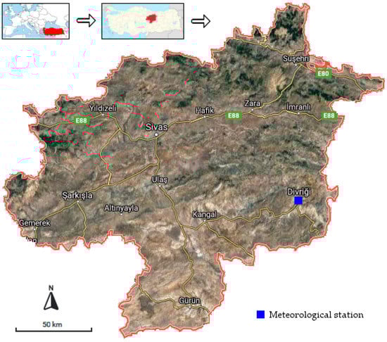
Figure 1. Study region.

Daily data measured in Turkish State Meteorological Service Sivas Divrigi station between 15 September 2009 and 31 December 2018 were used in the study. Measurements in the meteorological stations operated by the State Meteorological Service in Turkey are conducted according to standards set by the World Meteorological Organization. Measurements made manually in previous years are now made through automatic stations. Automatic meteorology stations consist of sensors sensitive to changes in meteorological parameters and measuring the amount of these changes. These stations have the main (central) processing unit that makes the necessary calculations to convert the measurements obtained by the sensors into meteorological information, the display units that enable the information to be displayed, and the communication units that enable the information to be transmitted to the center. The station also has a data acquisition unit, communication interface, and power supply [33,34].

Basic statistics about the data used are given in Table 1. Soil temperature values at a depth of 5 cm vary greatly compared to soil temperature values of 10 cm and 20 cm. The daily change of the average soil temperature at different depths throughout the year is given in Figure 2. In a sense, the change between the minimum and maximum temperature values is high. The testing was performed using the 70–30 report between training and test data. Data were split chronologically. Initial data had 3395 records. It was used in two separate repositories: the first 70% in the Training Data repository, between September 2009 and March 2016, was used to train the model, while the next 30% part, from March 2016 until December 2018, in the Test Data repository was used for validating it. These two repositories were used in all the created processes. We evaluated the best method and scenario for each of the proposed algorithms in order to implement and run a process that covered all the decided scenarios.

Table 1. Statistical properties of daily data related to air and soil.

Statistic	ST5 (°C)	ST10 (°C)	ST20 (°C)	MinT (°C)	MeanT (°C)	MaxT (°C)	Sunshine Intensity (cal/cm2)	Sunshine Duration (h)	Precip. (mm)
Minimum	−9.3	−8.4	−4.6	−19.8	−15.5	−11.3	0	0	0
Maximum	41.6	36.6	31.2	26.3	31.7	41.1	750.78	13.1	33.6
Mean	14.53	14.34	14.34	6.47	12.41	19.09	383.66	7.12	1.02
Stdev	11.12	10.53	9.73	8.18	9.66	11.30	200.12	4.09	3.10
Number of records	3316	3347	3347	3358	3358	3367	3275	3345	3395

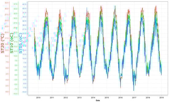
Figure 2. Average soil temperature change at different depths.

2.2. Methods

The data mining processes were implemented in Rapid Miner Studio (version 9.4–Educational Edition, RapidMiner Inc., Boston, MA, USA). It is a tool that provides a comprehensive set of operators and offers easy to use and understand structures for modelling complex data mining processes [35]. The machine-learning algorithms used for predicting the soil temperature are described below.

2.2.1. Gradient Boosted Trees (GBT)

Gradient boosted trees consists of an ensemble of regression/classification tree models. In the scenarios that we want to test, it is used for regression. According to Freund and Schapire [36], regression GBT is a generalization of boosting to arbitrary differentiable loss functions. These are learned in a sequential manner by a forward stagewise procedure [37]. The GBT implementation in Rapid Miner uses the H2O 3.8.2.6 algorithm. This follows the algorithm that was specified by Hastie et al. [38].

2.2.2. Decision Trees (DT)

Decision trees (DT)—a tree like a collection of nodes used to predict the affiliation to a class or an estimate of a numerical target value. Each node corresponds to a splitting rule for one specific attribute. This is a simple and widely used method in data mining [39].

The output of the model is a tree model, which is later used for prediction. The minimization of the sum of squares is used as a criterion.

As Hastie et al. [38] specified, the tree size will influence the resulted model complexity and the optimal size of the tree should be adaptively chosen. The correspondence for the tree size in Rapid Miner is “maximal depth” for which we tried different values in the optimization part.

2.2.3. Hybrid DT–GBT

The proposed hybrid DT–GBT approach uses the vote operator capabilities offered by Rapid Miner. It is a nested operator, meaning it has a subprocess. It also requires at least two learners, called base learners.

For classification, this operator uses a majority vote, while for regression it uses the average on top of the predictions of the base learners provided in the subprocess. For classification, all the operators in the subprocess accept the given dataset and generate a classification model. For predicting an unknown example, this operator applies all the classification models from its subprocess and assigns the predicted class with maximum votes to the unknown example.

In case of regression, all the operators in the subprocess of the vote operator accept the given dataset and generate a regression model. In the proposed hybrid DT–GBT approach, GBT and DT are included in the subprocess and are considered base learners. To predict an unknown value, the operator uses the average on top of the predictions of the base learners defined.

2.2.4. Metrics Performed for Evaluation

Five different well-known metrics calculated for evaluating the models (Equations (1) and (2)).

• Root mean squared error (RMSE)—the standard deviation of the residuals (prediction errors).
• Pearson correlation coefficient (r)—used to obtain the strength and direction of the linear relationship between the predicted value and observed value for the soil temperature.
• Mean absolute error (MAE)—it is commonly used in forecasting time series.
• Nash–Sutcliffe coefficient (NS)—used to describe the accuracy of model outputs:

  $$\mathrm{NS}=1-\frac{{\sum }_{i=1}^n{\left(p_i-d_i\right)}^2}{{\sum }_{i=1}^n{\left(p_i-\overline{p}\right)}^2},$$

  (1)

  where n is the number of outputs, p_i is the i-th predicted output, and d_i is the i-th desired observed output [40,41].
• Kling–Gupta efficiency (KGE)—first introduced by Gupta et al. [42] as an improvement to the Nash–Sutcliffe efficiency. It facilitates the separate analysis of the relative importance of correlation, bias, and variability in the process of hydrological modelling.

  $$\begin{array}{c}\mathrm{KGE}=1-\sqrt{{\left(r-1\right)}^2+{\left(\frac{{\sigma }_{\mathrm{sim}}}{{\sigma }_{\mathrm{obs}}}-1\right)}^2+{\left(\frac{{\mu }_{\mathrm{sim}}}{{\mu }_{\mathrm{obs}}}-1\right)}^2,}\end{array}$$

  (2)

  where r is the linear correlation between observed and predicted values, σ_obs is the standard deviation in observations, σ_sim the standard deviation in simulations, μ_sim the simulation mean, and μ_obs the observation mean.

2.2.5. Parameter Setup

To predict the soil temperature at different depths, the time windowing technique was used on the input data. Windowing is used to split time series into input vectors. A time series is a set of measurements performed on a specific process that are registered sequentially in time. As Koskela et al. [43] point out, by using the windowing technique, the problem is translated into deciding the length and type of the window to be used.

2.2.6. Scenarios and Implementation

In the study, 8 different input scenarios were taken into account to determine the meteorological variables that have the most impact on soil temperature and to evaluate the predictive power of the prediction models to be used based on these variables. The scenarios in Table 2 are based on the physics of soil temperature change and a literature search.

Table 2. Scenarios used and input variables.

Scenario	Meteorological Variables
1	MinT-MaxT-MeanT-Sunshine Intensity-Sunshine Duration-Precipitation
2	MinT-MaxT-MeanT-Sunshine Intensity-Sunshine Duration
3	MinT-MaxT-MeanT-Sunshine Duration
4	MinT-MaxT-MeanT-Sunshine Intensity
5	Sunshine Intensity-Sunshine Duration
6	MinT-MaxT-MeanT
7	MeanT-Sunshine Duration
8	MeanT

For validating the best combination for the machine-learning algorithms, a particularization of the configurable scenarios platform for designing prediction models, described in Avram et al. [44] and Avram et al. [45] was used, if the platform was thought to be general enough to support collaborative and context-aware data mining. As Anton et al. [46] specify, context-aware data mining respects the same steps as classical data mining, just that it includes real-time context in the data mining process, while the collaborative scenario involves having the data of the studied source completed with data taken from similar sources (for example one or more locations in close proximity to the studied one). In the current research, the focus was on the classical data mining approach, applied in the DT, GBT, and hybrid DT–GBT methods.

Below are the steps describing the modelled process behind each machine-learning method. Since there were three chosen models: DT, GBT, and hybrid DT–GBT, there were 3 Rapid Miner processes, following the presented structure:

• load training data;
• load testing data;
• load test scenarios;
• for each test scenario in the list:

  ○

  establish predicted value as specified in the scenario;

  ○

  select only attributes specified;

  ○

  generate model on the training data using windowing;

  ○

  apply generated model on the test data;

  ○

  store results.

• aggregate results.

The aggregated results were then subject to analysis, and conclusions were drawn based on these.

3. Results

To predict the soil temperature at different depths (5 cm, 10 cm, and 20 cm), the machine-learning algorithms were trained using windows of previous days. For establishing the best values for the window size, the values 3, 5, and 7 were tested in the beginning of the experiments. Table 3 presents the RMSE (°C) measured values per each algorithm used. It can be observed that the best results were obtained when using a window of 3 previous days, while increasing the number of days in the window did not improve the results.

Table 3. RMSE (°C) values for different values for window size per algorithm—with bold the lowest values.

Window Value/Algorithm	3	5	7
DT	1.3937	1.4219	1.4209
GBT	2.0939	2.0982	2.1058
Hybrid DT–GBT	1.8491	1.9546	1.9622

Table 4 presents the obtained results for different maximal depth values. We used in the experiments the maximal depth of 10 for the decision tree algorithm applied. For a maximal depth higher than 10, the overall accuracy of the predictions starts to decrease.

Table 4. RMSE values for different values for decision tree maximal depth.

Value for Maximal Depth	Avg RMSE Per Scenario (°C)
3	3.8837
5	2.6878
7	2.2810
10	2.2010
15	2.3768
20	2.2789

Table 5 depicts the results obtained for the combinations tested for GBT on maximal depth and no. of trees. After this phase, the combination 200 trees and 20 as maximal depth was further used in the experiments. For the hybrid DT–GBT approach, the best obtained parameters were used for each algorithm.

Table 5. RMSE (°C) values for different values for gradient boosted trees number of trees and maximal depth. Background color for emphasizing 3 main groups.

No of Trees	Max Depth	RMSE	No of Trees	Max Depth	RMSE	No. of Trees	Max Depth	RMSE
30	10	8.0326	100	10	4.3900	200	10	2.4910
30	20	8.0313	100	20	4.3869	200	20	2.4892
30	30	8.0313	100	30	4.3869	200	30	2.4893
50	10	6.6889	150	10	3.1269
50	20	6.6864	150	20	3.1240
50	30	6.6864	150	30	3.1240

In the study, the performance of the models and input scenarios used to estimate the temperature at different soil depths were determined. 70% of all data used in the study were used for training of models and the remaining 30% were used for testing.

RMSE (°C) was computed for all scenarios and algorithms chosen, as seen in Table 6. The results with the lowest RMSE were considered as best scenario combinations and analyzed in more details.

Table 6. RMSE results for all scenarios and algorithms chosen for ST5, ST10, and ST20—with bold the lowest values.

Scenario	Algorithm		RMSE (°C)
		ST5	ST10	ST20
MeanT	DT	2.0624	1.3795	0.8209
MeanT-Sunshine Duration	DT	2.0454	1.3379	0.7703
MinT-MaxT-MeanT	DT	2.0419	1.3677	0.7935
MinT-MaxT-MeanT-Sunshine Duration	DT	2.0289	1.3165	0.7368
MinT-MaxT-MeanT-Sunshine Intensity	DT	2.1041	1.3196	0.7522
MinT-MaxT-MeanT-Sunshine Int.-Sunshine Dur.	DT	2.1226	1.3306	0.7481
MinT-MaxT-MeanT-Sunshine Intensity-Sunshine Duration-Precipitation	DT	2.1271	1.3271	0.7479
Sunshine Intensity-Sunshine Duration	DT	2.0188	1.3790	0.7694
MeanT	GBT	2.6109	1.9734	1.6583
MeanT-Sunshine Duration	GBT	2.6495	1.9783	1.6505
MinT-MaxT-MeanT	GBT	2.6435	1.9674	1.6462
MinT-MaxT-MeanT-Sunshine Duration	GBT	2.6673	1.9554	1.6389
MinT-MaxT-MeanT-Sunshine Intensity	GBT	2.6686	1.9654	1.6509
MinT-MaxT-MeanT-Sunshine Int.-Sunshine Dur.	GBT	2.6785	1.9640	1.6480
MinT-MaxT-MeanT-Sunshine Intensity-Sunshine Duration-Precipitation	GBT	2.6803	1.9663	1.6473
Sunshine Intensity-Sunshine Duration	GBT	2.6521	2.0109	1.6807
MeanT	Hybrid	2.1007	1.4851	1.0770
MeanT-Sunshine Duration	Hybrid	2.1440	1.4334	1.0295
MinT-MaxT-MeanT	Hybrid	2.1609	1.4473	1.0445
MinT-MaxT-MeanT-Sunshine Duration	Hybrid	2.1505	1.4351	1.0121
MinT-MaxT-MeanT-Sunshine Intensity	Hybrid	2.1875	1.4432	1.0194
MinT-MaxT-MeanT-Sunshine Int.-Sunshine Dur.	Hybrid	2.1878	1.4375	1.0157
MinT-MaxT-MeanT-Sunshine Intensity-Sunshine Duration-Precipitation	Hybrid	2.2018	1.4366	1.0146
Sunshine Intensity-Sunshine Duration	Hybrid	2.1315	1.4417	1.0644

Seen in Table 7, which is only for best selected scenario for each depth given, the DT model was able to predict the soil temperature at a depth of 20, 10, and 5 cm, respectively. The soil temperature at a depth of 5 cm is predicted with a relatively high accuracy and low error (NS = 0.9669, KGE = 0.957, R = 0.9833, MAE = 1.4533 and RMSE = 2.0188). Soil temperature at a depth of 5 cm was more affected by the parameters of Sunshine Intensity and Sunshine Duration than other variables.

Table 7. Results of DT model at different depths.

Inputs	Output	NS	R	MAE	RMSE	KGE
Sunshine Intensity-Sunshine Duration	ST5	0.9669	0.9833	1.4533	2.0188	0.975
MinT-MaxT-MeanT-Sunshine Duration	ST10	0.9846	0.9922	0.9564	1.3165	0.989
MinT-MaxT-MeanT-Sunshine Duration	ST20	0.9942	0.9971	0.5171	0.7368	0.995

In Table 7, the soil temperature at 10 and 20 cm depth was mostly affected by MinT-MaxT-MeanT-Sunshine Duration parameters. The DT model had high accuracy and low error in soil temperature at 10 and 20 cm depth (ST10: NS = 0.9846, KGE = 0.989, R = 0.9922, MAE = 0.9564, RMSE = 1.3165 and ST20: NS = 0.9942, KGE = 0.995, R = 0.9971, MAE = 0.5171, RMSE = 0.7368). As the depth increases according to the evaluation criteria, the accuracy rate of the model has increased, and the margin of error has decreased.

Time series and scatter plots for all three depths are given in Figure 3. The DT model has successfully estimated the soil temperature at different depths.

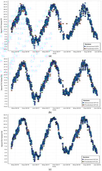
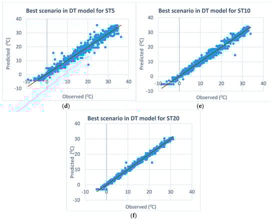
Figure 3. Comparison of observed and predicted: (a) soil temperatures at 5 cm depth; (b) soil temperatures at 10 cm depth; (c) soil temperatures at 20 cm depth; (d) best scenario for ST5; (e) best scenario for ST10 and (f) best scenario for ST20, 10, and 20 cm depth according to DT model.

In Table 8, the performance of the inputs and scenarios that give the best results for 5, 10, 20 cm soil depths according to the GBT model is given. The best estimates in GBT method were for 20, 10, and 5 cm depths, respectively, as in the DT method.

Table 8. Results of GBT model at different depths.

Inputs	Output	NS	R	MAE	RMSE	KGE
MeanT	ST5	0.9446	0.9793	1.9144	2.6109	0.857
MinT-MaxT-MeanT-Sunshine Duration	ST10	0.9658	0.9915	1.5442	1.9554	0.861
MinT-MaxT-MeanT-Sunshine Duration	ST20	0.9713	0.9939	1.2689	1.6389	0.866

In Table 8, it is sufficient to use the MeanT variable as an input to determine the temperature at a depth of 5 cm (NS = 0.9446, KGE = 0.857, R = 0.9793, MAE = 1.9144, RMSE = 2.6109). However, the input scenario consisting of four variables (MinT-MaxT-MeanT-Sunshine Duration) gave the best results for 10 and 20 cm soil depth. As seen in Table 8, the best results are 10 cm deep (NS = 0.9658, KGE = 0.861, R = 0.9915, MAE = 1.5442, RMSE = 1.9554) and 20 cm deep (NS = 0.9713, KGE = 0.866, R = 0.9939, MAE = 1.2689, RMSE = 1.6389). The success rate of the model increased as the depth of the soil increased in the GBT method.

According to the results of the GBT model, the time series and scatter plots for all three depths are given in Figure 4. A very high level of agreement was achieved between the values predicted from the GBT model and the observed values at all depths except for a few days.

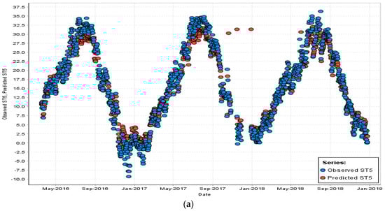
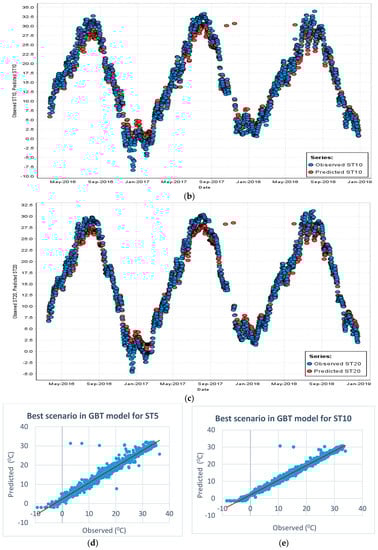
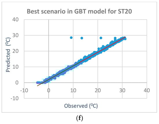
Figure 4. Comparison of observed and predicted: (a) soil temperatures at 5 cm depth; (b) soil temperatures at 10 cm depth; (c) soil temperatures at 20 cm depth; (d) best scenario for ST5; (e) best scenario for ST10 and (f) best scenario for ST20Comparison of observed and predicted soil temperatures at 5, 10, and 20 cm depth according to the GBT model.

In Table 9, the performance of the input scenarios that give the best results for temperatures at 5, 10, and 20 cm soil depths according to the DT–GBT hybrid model is given.

Table 9. Results of DT–GBT model at different depths.

Inputs	Output	NS	R	MAE	RMSE	KGE
MeanT	ST5	0.9642	0.9839	1.5358	2.1007	0.921
MeanT-Sunshine Duration	ST10	0.9817	0.9934	1.1025	1.4334	0.922
MinT-MaxT-MeanT-Sunshine Duration	ST20	0.9890	0.9968	0.7779	1.0121	0.930

In Table 9, the best result was obtained when the temperature of 5 cm soil depth was taken as the input of the MeanT variable only (NS = 0.9642, KGE = 0.921, R = 0.9839, MAE = 1.5358, RMSE = 2.1007). The input scenario consisting of two variables (MeanT-Sunshine Duration) for a depth of 10 cm gave the best results. For 20 cm depth, the input scenario consisting of four variables (MinT-MaxT-MeanT-Sunshine Duration) gave the best results. Seen in Table 9, at 10 cm deep NS = 0.9817, KGE = 0.922, R = 0.9934, MAE = 1.1025, RMSE = 1.4334 and at 20 cm deep NS = 0.9890, KGE = 0.930, R = 0.9968, MAE = 0.7779, RMSE = 1.0121 values were obtained. The results seen in Table 9 show that, as soil depth increases, the accuracy rate of the model also increases.

According to the DT–GBT hybrid model results, time series graphics and scatter plots for all three depths are given in Figure 5. Except for a few days, especially at 10 cm and 20 cm depths, a very high agreement was observed between the values estimated from the DT–GBT hybrid model and the observed values.

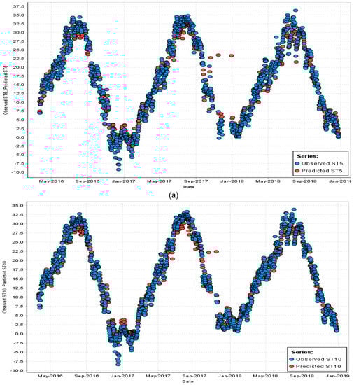
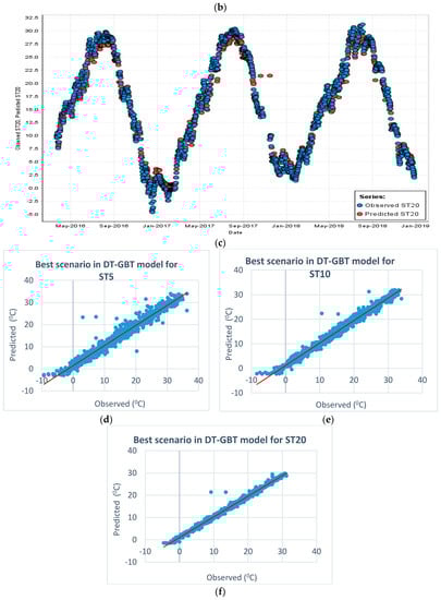
Figure 5. Comparison of observed and predicted: (a) soil temperatures at 5 cm depth; (b) soil temperatures at 10 cm depth; (c) soil temperatures at 20 cm depth; (d) best scenario for ST5; (e) best scenario for ST10 and (f) best scenario for ST20 Comparison of observed and predicted soil temperatures at 5, 10s and 20 cm depth according to the DT–GBT model.

The methods used in the continuation of the study were compared with each other for different depths.

The performance of the methods in test period for a depth of 5 cm is given in Table 10. In Table 10, the basic statistical values of the three different methods in the best successful scenarios can be compared with the measured values. The results obtained from the methods used are in the second, third, and fourth columns; in the last column, the figures for the measured values are given. The DT–GBT hybrid method with 5 cm depth in terms of R value gave more accurate results than other methods (R = 0.9954). However, DT was accurate in terms of minimum, maximum, and standard deviation values; in terms of mean value, it is seen that the results of GBT method are close to the observed temperature values. In general, it has been proved that all three methods can predict accurate soil temperature at a depth of 5 cm.

Table 10. Statistic for selected scenarios in used methods ST5.

Methods	DT	GBT	Hybrid DT–GBT	Measured (ST5)
Best Scenario	Sunshine Intensity, Sunshine Duration	MeanT	MeanT
Minimum	−4.21	−2.00	−3.03	−9.30
Maximum	35.55	32.05	33.95	41.60
Mean	16.29	16.12	16.29	14.53
Stdev	10.89	9.54	10.25	11.12
Correlation	0.9800	0.9923	0.9954	1.0000
Number of records	965	965	965	3316

The performance of the methods in the test period for the prediction of the soil temperature 10 cm deep is given in Table 11. In terms of R value, the DT method with a depth of 10 cm was more accurate than other methods (R = 0.9983). At the same time, the DT method results are very close to observed temperature values in terms of minimum, maximum, mean, and standard deviation values. In this case, it was proved that all three methods successfully predicted soil temperature at 10 cm deep.

Table 11. Statistic for selected scenarios in used methods ST10.

Methods	DT	GBT	Hybrid DT–GBT	Measured (ST10)
Best Scenario	MinT-MaxT-MeanT-Sunshine Duration	MinT-MaxT-MeanT-Sunshine Duration	MeanT-Sunshine Duration
Minimum	−5.25	−1.43	−2.28	−8.40
Maximum	33.83	30.70	31.95	33.90
Mean	15.80	15.62	15.73	15.84
Stdev	10.50	9.12	9.77	10.58
Correlation	0.9983	0.9900	0.9900	1.0000
Number of records	998	998	998	3347

The performance of the methods in test period for a depth of 20 cm is given in Table 12. In terms of the R value, DT method with a depth of 20 cm showed better results with a little difference compared to other methods (R = 0.9994). At the same time, the DT method results are very close to observed temperature values in terms of minimum, maximum, mean, and standard deviation values. The DT method is very closely followed by the hybrid DT–GBT method. In this case, it was proved that all three methods successfully predicted soil temperature at 20 cm deep.

Table 12. Statistic for selected scenarios in used methods ST20.

Methods	DT	GBT	Hybrid DT–GBT	Measured (ST20)
Best Scenario	MinT-MaxT-MeanT-Sunshine Duration	MinT-MaxT-MeanT-Sunshine Duration	MinT-MaxT-MeanT-Sunshine Duration
Minimum	−2.95	−0.06	−1.47	−4.60
Maximum	31.02	28.53	29.78	31.20
Mean	15.739	15.56	15.68	15.79
Stdev	9.6425	8.38	9.00	9.66
Correlation	0.9994	0.9933	0.9974	1.0000
Number of records	998	998	998	3347

It can be understood from Table 10, Table 11 and Table 12 that the sunshine duration affects the soil temperature, especially at 10 and 20 cm depth compared to other meteorological variables. It is seen that the sunshine duration time variable is the most important variable, since it causes the soil to heat. After the sunshine duration meteorological variable, it is seen that it plays an important role in soil warming, especially at 5 cm depth, in other variables that express the air temperature.

The performance of the models used for different depths is given visually as a Taylor diagram in Figure 6. As can be seen from Figure 6a, hybrid DT–GBT, GBT, and DT methods have best predicted soil temperature at 5 cm soil depth, respectively. As seen in Figure 6b,c, the best results in soil temperature estimation at 10 and 20 cm soil depths were obtained with DT, hybrid DT–GBT, and GBT methods, respectively.

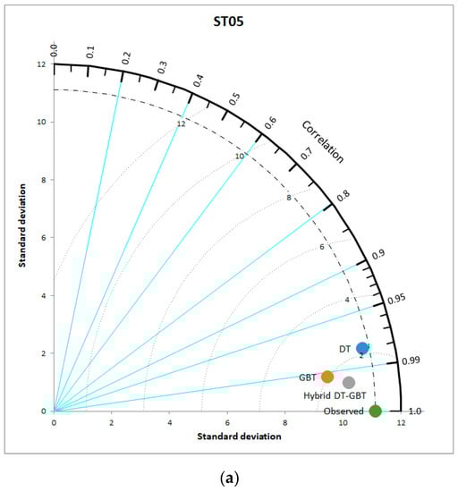
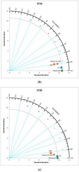
Figure 6. Taylor diagrams of the models used for different depths. (a) 5 cm depth; (b) 10 cm depth; (c) 20 cm depth.

4. Discussion

Estimation of soil temperature is one of the most important factors in the management of economic activities, such as agriculture and construction and agricultural insurance. Soil temperature is a factor that depends on meteorological variables and can be measured at meteorological stations, but it requires a relatively high cost, with expert staff.

Unfortunately, many meteorological parameters have measured at only one location in Turkey’s district, such as Divrigi, except metropolitan areas. The transferability of the data mining model trained at a single point is likely to be low. However, the altitude change is not very high in the district, and there are no other long-term measuring stations. Naturally, the results obtained here cannot be generalized for other regions and other conditions.

The evaluation criteria were taken into account in the selection of the best scenario and the best model. The accuracy rate obtained under these operating conditions is quite good (NS: 0.9446–0.9942, KGE: 0.857–0.995, R: 0.9793–0.9971). Accuracy rate in all data-based models can be increased by discovering hidden patterns and minimizing the noise in the data. It is possible to make data smoother and more predictable with data preprocessing. With various preprocessing and filtering methods, the stochastic feature among the data can be reduced, and the accuracy of the model can be increased.

Using data-based models, soil temperature can be estimated at different depths with meteorological variables measured in the past. In this study, the performance of the hybrid DT–GBT method developed with DT and GBT methods in estimating soil temperature at different depths was compared. While estimating the soil temperature, the meteorological variables associated with the temperature were considered as input scenarios in eight different combinations. According to the results, the hybrid DT–GBT, GBT, and DT methods were best predicted at 5 cm soil depth, respectively. In 10 and 20 cm soil depths, the best estimate was obtained by DT, hybrid DT–GBT, and GBT models, respectively. At the same time, it was observed that the accuracy rate of the models increased with increasing soil depth. It was observed that the sunshine duration was the most important meteorological variable for soil temperature at 10 and 20 cm depth and the air temperature was the most important at 5 cm soil depth. It was observed that precipitation was ineffective on soil temperature in all models and at all depths. As a result, the DT, GBT, and hybrid DT–GBT models have been used successfully for predicting soil temperature.

Soil temperature is important for plant root development and the activity of microorganisms. It is not possible to measure this temperature at different depths, especially in the field conditions where vegetative production is made, because it is a costly process that requires equipment and expert staff. However, if successful models can be established for different regions and conditions, the soil temperature can be predicted without the need for land measurement, equipment, or labor. These predictions can assist in agricultural soil, fertilizer, and water resources management. Although three different artificial intelligence methods were used in this study, we did not have the chance to test them in different climatic and regional conditions. It cannot be generalized that the proposed model that makes the best estimates will be valid in all conditions, but it has been concluded that the methods can be used in the estimation of the soil temperature due to the successful results.

References

- Bond-Lamberty, B.; Wang, C.; Gower, S.T. Spatiotemporal measurement and modeling of stand-level boreal forest soil temperatures. Agric. For. Meteorol. 2005, 131, 27–40. [Google Scholar] [CrossRef]
- Buckman, H.O.; Brady, N.C. The Nature and Properties of Soils, 6th ed.; The Mac Millian Co.: New York, NY, USA, 1960. [Google Scholar]
- Seyfried, M.S.; Flerchinger, G.N.; Murdock, M.D.; Hanson, C.L.; Van Vactor, S. Long-Term Soil Temperature Database, Reynolds Creek Experimental Watershed, Idaho, United States. Water Resour. Res. 2001, 37, 2843–2846. [Google Scholar] [CrossRef]
- Tenge, A.; Kaihura, F.B.; Lal, R.; Singh, B. Diurnal soil temperature fluctuations for different erosion classes of an oxisol at Mlingano, Tanzania. Soil Tillage Res. 1998, 49, 211–217. [Google Scholar] [CrossRef]
- Zheng, D.; Hunt, E.; Running, S. A daily soil temperature model based on air temperature and precipitation for continental applications. Clim. Res. 1993, 2, 183–191. [Google Scholar] [CrossRef]
- Yang, C.-C.; Prasher, S.O.; Mehuys, G.R.; Patni, N.K. Application of artificial neural networks for simulation of soil temperature. Trans. ASAE 1997, 40, 649–656. [Google Scholar] [CrossRef]
- Paul, K.I.; Polglase, P.J.; Smethurst, P.J.; O’Connell, A.M.; Carlyle, C.J.; Khanna, P.K. Soil temperature under forests: A simple model for predicting soil temperature under a range of forest types. Agric. For. Meteorol. 2004, 121, 167–182. [Google Scholar] [CrossRef]
- Bilgili, M. Prediction of soil temperature using regression and artificial neural network models. Meteorol. Atmos. Phys. 2010, 110, 59–70. [Google Scholar] [CrossRef]
- Sattari, M.T.; Apaydin, H.; Shamshirband, S. Performance Evaluation of Deep Learning-Based Gated Recurrent Units (GRUs) and Tree-Based Models for Estimating ETo by Using Limited Meteorological Variables. Mathematics 2020, 8, 972. [Google Scholar] [CrossRef]
- Sattari, M.T.; Dodangeh, E.; Abraham, J. Estimation of daily soil temperature via data mining techniques in semi-arid climate conditions. Earth Sci. Res. J. 2017, 21, 85–93. [Google Scholar] [CrossRef]
- Apaydin, H.; Feizi, H.; Sattari, M.T.; Colak, M.S.; Shamshirband, S.; Chau, K.-W. Comparative Analysis of Recurrent Neural Network Architectures for Reservoir Inflow Forecasting. Water 2020, 12, 1500. [Google Scholar] [CrossRef]
- Keskiner, A.; Ibrikci, T.; Cetin, M. Estimation and Comparison of Probabilistic Temperatures through Using Artificial Neural Networks in Geographic Information Systems Media. J. Agric. Sci. 2012, 17, 242–252. [Google Scholar]
- Yurekli, K.; Sattari, M.T.; Anli, A.S.; Hinis, M.A. Seasonal and annual regional drought prediction by using data-mining approach. Atmosfera 2012, 25, 85–105. [Google Scholar]
- Terzi, O.; Barak, M. Rainfall-Runoff Forecasting with Wavelet-Neural Network Approach: A Case Study of Kızılırmak River. J. Agric. Sci. 2015, 21, 546–557. [Google Scholar]
- Nourani, V.; Sattari, M.T.; Molajou, A. Threshold-Based Hybrid Data Mining Method for Long-Term Maximum Precipitation Forecasting. Water Resour. Manag. 2017, 31, 2645–2658. [Google Scholar] [CrossRef]
- Sattari, M.T.; Mirabbasi, R.; Sushab, R.S.; Abraham, J.P. Prediction of Groundwater Level in Ardebil Plain Using Support Vector Regression and M5 Tree Model. Ground Water 2018, 56, 636–646. [Google Scholar] [CrossRef]
- Rouzegari, N.; Hassanzadeh, Y.; Sattari, M.T. Using the Hybrid Simulated Annealing-M5 Tree Algorithms to Extract the If-Then Operation Rules in a Single Reservoir. Water Resour. Manag. 2019, 33, 3655–3672. [Google Scholar] [CrossRef]
- Shabani, S.; Samadianfard, S.; Sattari, M.T.; Mosavi, A.; Shamshirband, S.; Kmet, T.; Várkonyi-Kóczy, A.R. Modeling Pan Evaporation Using Gaussian Process Regression K-Nearest Neighbors Random Forest and Support Vector Machines; Comparative Analysis. Atmosphere 2020, 11, 66. [Google Scholar] [CrossRef]
- Zounemat-Kermani, M. Hydrometeorological Parameters in Prediction of Soil Temperature by Means of Artificial Neural Network: Case Study in Wyoming. J. Hydrol. Eng. 2013, 18, 707–718. [Google Scholar] [CrossRef]
- Aslay, F.; Ozen, U. Estimating Soil Temperature with Artificial Neural Networks Using Meteorological Parameters. J. Polytech. 2013, 16, 139–145. [Google Scholar]
- Hosseinzadeh Talaee, P. Daily soil temperature modeling using neuro-fuzzy approach. Theor. Appl. Climatol. 2014, 118, 481–489. [Google Scholar] [CrossRef]
- Kim, S.; Singh, V.P. Modeling daily soil temperature using data-driven models and spatial distribution. Theor. Appl. Climatol. 2014, 118, 465–479. [Google Scholar] [CrossRef]
- Yener, D.; Ozgener, O.; Ozgener, L. Prediction of soil temperatures for shallow geothermal applications in Turkey. Renew. Sustain. Energy Rev. 2017, 70, 71–77. [Google Scholar] [CrossRef]
- Samadianfard, S.; Asadi, E.; Jarhan, S.; Kazemi, H.; Kheshtgar, S.; Kisi, O.; Sajjadi, S.; Manaf, A.A. Wavelet neural networks and gene expression programming models to predict short-term soil temperature at different depths. Soil Tillage Res. 2018, 175, 37–50. [Google Scholar] [CrossRef]
- Feng, Y.; Cui, N.; Hao, W.; Gao, L.; Gong, D. Estimation of soil temperature from meteorological data using different machine learning models. Geoderma 2019, 338, 67–77. [Google Scholar] [CrossRef]
- Costache, R.; Pham, Q.B.; Avand, M.; Thuy Linh, N.T.; Vojtek, M.; Vojteková, J.; Lee, S.; Khoi, D.N.; Thao Nhi, P.T.; Dung, T.D. Novel hybrid models between bivariate statistics, artificial neural networks and boosting algorithms for flood susceptibility assessment. J. Environ. Manag. 2020, 265, 110485. [Google Scholar] [CrossRef] [PubMed]
- Matei, O.; Rusu, T.; Petrovan, A.; Mihut, G. A data mining system for real time soil moisture prediction. Procedia Eng. 2017, 181, 837–844. [Google Scholar] [CrossRef]
- Matei, O.; Rusu, T.; Bozga, A.; Pop, P.; Anton, A. Context-aware data mining: Embedding external data sources in a machine learning process. In International Conference on Hybrid Artificial Intelligence Systems; Springer: Cham, Switzerland, 2017. [Google Scholar] [CrossRef]
- Anton, C.A.; Avram, A.; Petrovan, A.; Matei, O. Performance Analysis of Collaborative Data Mining vs Context Aware Data Mining in a Practical Scenario for Predicting Air Humidity. In Proceedings of the Computational Methods in Systems and Software; Springer: Cham, Switzerland, 2019; pp. 31–40. [Google Scholar] [CrossRef]
- Wu, Z.; Zhou, Y.; Wang, H.; Jiang, Z. Depth prediction of urban flood under different rainfall return periods based on deep learning and data warehouse. Sci. Total Environ. 2020, 716, 137077. [Google Scholar] [CrossRef]
- Anoynmous. Sivas Investment Guide; Central Anatolia Development Agency: Kayseri, Turkey, 2017. (In Turkish)
- Anoynmous. Activity Report; Republic of Turkey, Sivas Governorship Agriculture and Forest Provincial Directorate: Sivas, Turkey, 2019. (In Turkish)
- Anoynmous. Meteorological Instruments; State Meteorological Service. Available online: https://www.mgm.gov.tr/genel/meteorolojikaletler.aspx (accessed on 8 August 2020). (In Turkish)
- Anoynmous. Specifications of Meteorological Instruments; State Meteorological Service. Available online: https://www.mgm.gov.tr/FILES/kurumsal/mevzuat/ruzgar-gunes-ek.pdf (accessed on 8 August 2020). (In Turkish)
- Hofmann, M.; Klinkenberg, R. RapidMiner: Data Mining Use Cases and Business Analytics Applications; CRC Press: Boca Raton, FL, USA, 2016. [Google Scholar]
- Freund, Y.; Schapire, R.E. A decision-theoretic generalization of on-line learning and an application to boosting. In European Conference on Computational Learning Theory; Springer: Berlin/Heidelberg, Germany, 1995; pp. 23–37. [Google Scholar]
- Breiman, L.; Friedman, J.; Stone, C.J.; Olshen, R.A. Classification and Regression Trees; CRC Press: Boca Raton, FL, USA, 1984. [Google Scholar]
- Hastie, T.; Tibshirani, R.; Friedman, J. The Elements of Statistical Learning: Data Mining, Inference, and Prediction; Springer Science & Business Media: Berlin/Heidelberg, Germany, 2009. [Google Scholar]
- Rokach, L.; Oded, Z.M. Data Mining with Decision Trees: Theory and Applications; World Scientific: Singapore, 2008; Volume 69. [Google Scholar]
- Nash, J.E.; Sutcliffe, J.V. River flow forecasting through conceptual models part I—A discussion of principles. J. Hydrol. 1970, 10, 282–290. [Google Scholar] [CrossRef]
- Hyndman, R.J.; Koehler, A.B. Another look at measures of forecast accuracy. Int. J. Forecast. 2006, 22, 679–688. [Google Scholar] [CrossRef]
- Gupta, H.V.; Kling, H.; Yilmaz, K.K.; Martinez, G.F. Decomposition of the mean squared error and NSE performance criteria: Implications for improving hydrological modelling. J. Hydrol. 2009, 377, 80–91. [Google Scholar] [CrossRef]
- Koskela, T.; Markus, V.; Jukka, H.; Kimmo, K. Timeseries prediction using recurrent som with local linear models. Int. J. Knowl. Based Intell. Eng. Syst. 1998, 2, 60–68. [Google Scholar]
- Avram, A.; Matei, O.; Pintea, C.; Pop, P.; Anton, C. Context-aware data mining vs classical data mining: Case study on predicting soil moisture. In International Workshop on Soft Computing Models in Industrial and Environmental Applications; Springer: Cham, Switzerland, 2019. [Google Scholar] [CrossRef]
- Avram, A.; Matei, O.; Pintea, C.; Anton, C. Innovative Platform for Designing Hybrid Collaborative Context-Aware Data Mining Scenarios. Mathematics 2020, 8, 684. [Google Scholar] [CrossRef]
- Anton, C.A.; Matei, O.; Avram, A. Collaborative Data Mining in Agriculture for Prediction of Soil Moisture and Temperature. Computer Science On-Line Conference; Springer: Cham, Switzerland, 2019. [Google Scholar] [CrossRef]
© 2020 by the authors. Licensee MDPI, Basel, Switzerland. This article is an open access article distributed under the terms and conditions of the Creative Commons Attribution (CC BY) license (http://creativecommons.org/licenses/by/4.0/).