State Observation for Lipschitz Nonlinear Dynamical Systems Based on Lyapunov Functions and Functionals

Abstract

State observers for systems having Lipschitz nonlinearities are considered for what concerns the stability of the estimation error by means of a decomposition of the dynamics of the error into the cascade of two systems. First, conditions are established in order to guarantee the asymptotic stability of the estimation error in a noise-free setting. Second, under the effect of system and measurement disturbances regarded as unknown inputs affecting the dynamics of the error, the proposed observers provide an estimation error that is input-to-state stable with respect to these disturbances. Lyapunov functions and functionals are adopted to prove such results. Third, simulations are shown to confirm the theoretical achievements and the effectiveness of the stability conditions we have established.

1. Introduction

Whenever there is the need to monitor the time behavior of internal system variables that are not accessible, observers are usually considered, but the demonstration of stability of the estimation error may be difficult to ensure whether the dynamic and measurement equations include nonlinear terms. Here, we address the problem of analyzing the input-to-state stability (ISS) of the estimation error for a class of Lipschitz nonlinear systems by using both Lyapunov functions and Lyapunov functionals, where the estimation error and system/measurement disturbances are regarded as state and input, respectively.

The first results dealing with observers for systems with nonlineartrace back to the beginning of the seventies [1,2]. The next works were focused on state transformations able to turn into a dynamics being linear in the new coordinates [3,4,5,6]. Variable-structure observers were proposed in [7,8] during the eighties but the big advance occurred later based on [9,10], where the nonlinearity in the dynamics of the estimation error is elegantly treated by using a high gain (see, for recent results [11,12], and the references therein). Therefore, these estimators are still denoted as “high-gain observers” and successfully employed for the purpose of output feedback control (see [13] and the references therein). Starting with [14,15], attention has been paid to the development of observers by taking advantage of suitable triangular structures due to a change in the state coordinates (see, e.g., [16]) and of effective methods of observer construction by accounting for disturbances affecting the system [17].

In this paper, novel results concerning the stability of the estimation error of observers for a class of systems with Lipschitz nonlinear terms are presented. The stability of the error is proved in by exploiting the ISS property of cascaded systems (see, for an overview, [18]). Such results are also proved by means of Lyapunov functions and functionals, in line with the previous literature [19,20,21,22,23] on the use of ISS to analyze the stability of the estimation error. The proposed observers may be designed by using linear matrix inequalities (LMIs) [24]. As compared with recent results on ISS for the stability analysis of state observers [25,26], the novel contribution concerns the investigation of Lyapunov functional instead of Lyapunov functions. This goal is pursued by resorting to the decomposition of the dynamics of the error, which holds for systems with Lipschitz nonlinearities. The use of the Schur complement and LMIs allow to overcome the difficulties to solve the Riccati equations (see, e.g., [27]) required to design the estimators.

The paper is structured, as follows. Section 2 presents the proposed class of observers and the related stability analysis in the absence and presence of disturbances, and a method of design relying on LMIs [28]. Section 3 illustrates the results that we achieved by simulations. Finally, conclusions and ideas for future work are summarized in Section 4.

We conclude this section with the following definitions. The symbol $|·|$ stands for the usual the Euclidean norm in ${\mathbb{R}}^n$. For a square matrix $S$, $S>0$ ($S<0$) indicates that this matrix is positive definite (negative definite); ${\lambda }_{\min }\left(S\right)$, and ${\lambda }_{\max }\left(S\right)$ denote the minimum and maximum eigenvalues of the symmetric positive or negative definite matrix $S$, respectively. The symbol “$\mathrm{ess}\sup$” denotes the essential supremum. The Schur complement provides the following equivalent conditions:

$$\begin{array}{c}\hfill \left(\begin{array}{cc}R& S\\ S^{\top }& T\end{array}\right)>0\mathrm{if}\mathrm{and}\mathrm{only}\mathrm{if}T>0,R-S{T}^{-1}{S}^{\top }>0\mathrm{if}\mathrm{and}\mathrm{only}\mathrm{if}R>0,T-S^{\top }{R}^{-1}S>0\end{array}$$

with $R,T$, and $S$ denoting square matrices and rectangular matrix, respectively [24]. A continuous function $\alpha :[0,a)\to [0,+\infty )$ is of class $\mathcal{K}$ if it is strictly increasing and $\alpha \left(0\right)=0$ and of class ${\mathcal{K}}_{\infty }$ if $a=+\infty$ and ${\displaystyle \underset{r\to +\infty }{lim}\alpha \left(r\right)=+\infty }$; a continuous function $\beta :[0,a)\times [0,+\infty )\to [0,+\infty )$ is of class $\mathcal{KL}$ if, for each fixed s, the mapping $\beta (r,s)$ belongs to class $\mathcal{K}$ with respect to $r$ and, for each fixed r, the mapping $\beta (r,s)$ is decreasing with respect to $s$ and ${\displaystyle \underset{s\to +\infty }{lim}\beta (r,s)=0}$.

2. Stability Analysis in a Noise-Free Case

Let us focus on nonlinear systems that are given by

$$\begin{array}{c}\dot{x}=Ax+f\left(x\right)\hfill \\ y=Cx\hfill \end{array},t\ge 0$$

(1)

where $x\left(t\right)\in X\subseteq {\mathbb{R}}^n$ is the state and $y\left(t\right)\in Y\subseteq {\mathbb{R}}^p$ is the output. The $n\times n$ matrix $A$ and the $p\times n$ matrix $C$ are given by

$$A=\mathrm{block}\mathrm{diag}\left(A_1,\cdots ,A_p\right)A_i=\left(\begin{array}{ccc}0& 1& 0\\ 0& 0& 1\\ ⋮& ⋮& ⋮& \ddots \\ 0& 0& 0& \cdots & 0& 1\\ 0& 0& 0& \cdots & 0& 0\end{array}\right)\in {\mathbb{R}}^{n_i\times n_i}$$

$$C=\mathrm{block}\mathrm{diag}\left(C_1,\cdots ,C_p\right)C_i=(10\cdots 0)\in {\mathbb{R}}^{n_i}$$

and ${\displaystyle \sum _{i=1}^p{n}_i=n}$. The solution of (1) exists and is unique for all $t\ge 0$ under the Lipschitz assumption for $x\mapsto f\left(x\right)$.

Assumption A1.

The function $f:X\to {\mathbb{R}}^n$ is Lipschitz in $x$, namely there exists $k_f>0$, such that

$$|f\left(x_1\right)-f\left(x_2\right)|\le k_f|x_1-x_2|$$

for all $x_1,x_2\in {\mathbb{R}}^n$.

Remark 1.

The proposed approach (detailed in the following) may be applied to a wider class of nonlinear, essentially observable systems being diffeomorphic to (1). Toward this end, in [29] conditions are presented to guarantee the existence of a diffeomorphism that turns nonlinear systems of quite general class into systems like that in (1). Therefore, an estimator for (1) becomes a stable observer in the original coordinate by using the inverse of this diffeomorphism.

Let us consider

$$\dot{\widehat{x}}=A\widehat{x}+f\left(\widehat{x}\right)+L\left(y-C\widehat{x}\right),t\ge 0$$

(2)

as full-order state observer for (1), where $\widehat{x}\left(t\right)\in {\mathbb{R}}^n$ is the estimate of $x\left(t\right)$ at time $t$ and $L\in {\mathbb{R}}^{n\times p}$ is a suitable gain matrix to select. The gain $L$ must be selected in such a way to make the estimation error $e\left(t\right):=x\left(t\right)-\widehat{x}\left(t\right)$ asymptotically stable. Thus, we analyze the dynamics of the estimation error, given by

$$\dot{e}=(A-LC)e+f\left(x\right)-f\left(\widehat{x}\right),t\ge 0$$

by decomposing $e\left(t\right)$ into two components that are given by $e_1\left(t\right)\in {\mathbb{R}}^n$ and $e_2\left(t\right)\in {\mathbb{R}}^n$ with $e\left(t\right)=e_1\left(t\right)+e_2\left(t\right)$ and

$$\begin{array}{c}{\mathsf{\Sigma }}_1:{\dot{e}}_1=(A-LC)e_1+f\left(x\right)-f(x-e_1-e_2)\hfill \\ {\mathsf{\Sigma }}_2:{\dot{e}}_2=(A-LC)e_2\hfill \end{array},t\ge 0$$

(3)

where $e_1\left(0\right)=0$ and $e_2\left(0\right)=e\left(0\right)$. Therefore, the stability of the observer is analyzed by studying the subsystems ${\mathsf{\Sigma }}_1$ and ${\mathsf{\Sigma }}_2$ in cascade.

Notice that, even if ${\mathsf{\Sigma }}_1$ is asymptotically stable with a null input, the asymptotic stability of ${\mathsf{\Sigma }}_2$ does not ensure the global stability. The stability of systems in cascade depends on the converging-input bounded-state (CIBS) property [30,31,32]. In case ${\mathsf{\Sigma }}_1$ with a zero input and ${\mathsf{\Sigma }}_2$ are globally asymptotically stable and ${\mathsf{\Sigma }}_1$ is CIBS, it follows that the cascade of ${\mathsf{\Sigma }}_1$ and ${\mathsf{\Sigma }}_2$ is globally asymptotically stable. To prove the results that are shown later, some technical lemmas are required.

Lemma 1.

Under Assumption 1, consider the system

$${\dot{e}}_1=(A-LC)e_1+f\left(x\right)-f(x-e_1)$$

(4)

where $e_1\left(t\right)\in {\mathbb{R}}^n$. Subsequently, independently of $x\left(t\right)$ given by (1), (4) is globally asymptotically stable if there exist $\alpha >0$, a gain matrix $L$, and a symmetric positive definite matrix $P$, such that

$$\begin{array}{c}\hfill \left(\begin{array}{cc}{(A-LC)}^{\top }P+P(A-LC)+\alpha k_f^{2}I& P\\ P& -\alpha I\end{array}\right)<0.\end{array}$$

(5)

Proof. 

As $|f\left(x\right)-f(x-e_1)|\le k_f\left|e_1\right|$, it turns out that $k_f^2{\left|e_1\right|}^2-{\left|f\left(x\right)-f(x-e_1)\right|}^2\ge 0$ for all x, $e_1\in {\mathbb{R}}^n$. Thus, consider the following Lyapunov functional

$$V=e_1^{\top }P{e}_1+\alpha {\int }_0^t{k}_f^2{\left|e_1\left(\tau \right)\right|}^2-{\left|f\left(x\left(\tau \right)\right)-f(x\left(\tau \right)-e_1\left(\tau \right))\right|}^{2}d\tau .$$

(6)

This functional is well-defined, as it is positive definite and equal to zero if and only if $e_1=0$. From (6), it follows that

$$\begin{array}{ccc}\hfill \dot{V}& =& e_1^{\top }\left[{(A-LC)}^{\top }P+P(A-LC)\right]e_1+e_1^{\top }P\left[f\left(x\right)-f(x-e_1)\right]+{\left[f\left(x\right)-f(x-e_1)\right]}^{\top }P{e}_1\hfill \\ & +& \alpha k_f^2{e}_1^{\top }{e}_1-\alpha {\left[f\left(x\right)-f(x-e_1)\right]}^{\top }\left[f\left(x\right)-f(x-e_1)\right]\hfill \end{array}$$

and so the derivative of $V$ is negative definite if (5) is satisfied. Moreover, note that ${\displaystyle \underset{e_1\to +\infty }{lim}V\left(e_1\right)=+\infty }$. As a consequence, one can apply the Barbashin–Krasivskii theorem (see, e.g., [33], Theorem 3.2, p. 110) to conclude the proof. □

Lemma 2.

Under Assumption 1, let us consider the system

$${\dot{e}}_1=(A-LC)e_1+f\left(x\right)-f(x-e_1-e_2)$$

(7)

where $e_1\left(t\right)\in {\mathbb{R}}^n$ with $e_1\left(0\right)=0$ and $e_2\left(t\right)\in {\mathbb{R}}^n$ are treated as state and input, respectively. Subsequently, independently of $x\left(t\right)$ solution of (1), there exists a compact set $K\subset {\mathbb{R}}^n$, such that $e\left(t\right)\in K$ for all $t\ge 0$ if $\alpha >0$, a gain matrix $L$, and a square matrix $P>0$ exist, such that

$$\begin{array}{c}\hfill \left(\begin{array}{cc}{(A-LC)}^{\top }P+P(A-LC)+\alpha k_f^{2}I& P\\ P& -\alpha I\end{array}\right)<0.\end{array}$$

(8)

Proof. 

First, note that it is necessary for $A-LC$ to be a Hurwitz matrix if (8) holds. Note that the Lyapunov functional

$$V=e_1^{\top }P{e}_1+\alpha {\int }_t^{+\infty }{\left|f\left(x\left(\tau \right)\right)-f(x\left(\tau \right)-e_2\left(\tau \right))\right|}^{2}d\tau .$$

(9)

is well-defined, as $0\le |f\left(x\right)-f(x-e_2)|\le k_f\left|e_2\right|$ and, since $A-LC$ is a Hurwitz matrix, $e_2\left(t\right)$ converges exponentially to zero. The time derivative of (9) is

$$\begin{array}{ll}\dot{V}& {\displaystyle =e_1^{\top }\left[{(A-LC)}^{\top }P+P(A-LC)\right]e_1+e_1^{\top }P\left[f\left(x\right)-f(x-e_1-e_2)\right]}\\ & +{\left[f\left(x\right)-f(x-e_1-e_2)\right]}^{\top }P{e}_1-\alpha {\left[f\left(x\right)-f(x-e_2)\right]}^{\top }\left[f\left(x\right)-f(x-e_2)\right].\end{array}$$

(10)

We have

$$\begin{array}{c}\hfill {\displaystyle |f\left(x\right)-f(x-e_1-e_2)|=|f\left(x\right)-f(x-e_2)+f(x-e_2)-f(x-e_1-e_2)|}\\ \le |f\left(x\right)-f(x-e_2)|+|f(x-e_2)-f(x-e_1-e_2)|\hfill \end{array}$$

(11)

and, hence, after applying a square to both sides of (11) and multiplying by $\alpha$, a little algebra yields

$$\begin{array}{c}{\displaystyle -\alpha |f\left(x\right)-f(x-e_2){|}^2\le -\alpha {|f\left(x\right)-f(x-e_1-e_2)|}^2}\hfill \\ +2\alpha |f\left(x\right)-f(x-e_2)\left|\right|f(x-e_2)-f(x-e_1-e_2)|+\alpha |f(x-e_2)-f(x-e_1-e_2){|}^2.\hfill \end{array}$$

By means of the above inequality, from (10) it follows that

$$\begin{array}{c}{\displaystyle \dot{V}\le e_1^{\top }\left[{(A-LC)}^{\top }P+P(A-LC)\right]e_1+e_1^{\top }P\left[f\left(x\right)-f(x-e_1-e_2)\right]}\hfill \\ +{\left[f\left(x\right)-f(x-e_1-e_2)\right]}^{\top }P{e}_1-\alpha {|f\left(x\right)-f(x-e_1-e_2)|}^2\hfill \\ +2\alpha |f\left(x\right)-f(x-e_2)\left|\right|f(x-e_2)-f(x-e_1-e_2)|+\alpha |f(x-e_2)-f(x-e_1-e_2){|}^2\hfill \end{array}$$

where the function $x\mapsto f\left(x\right)$ is Lipschitz from Assumption 1. Thus, the last two terms of the previous inequality can be bounded from above, as follows:

$$2\alpha |f\left(x\right)-f(x-e_2)\left|\right|f(x-e_2)-f(x-e_1-e_2)|\le 2\alpha k_f^2|e_1\left|\right|e_2|,$$

$$\alpha |f(x-e_2)-f(x-e_1-e_2){|}^2\le \alpha k_f^2{\left|e_1\right|}^2.$$

Thus, we have

$$\begin{array}{c}\hfill \dot{V}\le \left[e_1^{\top }{\left(f\left(x\right)-f(x-e_1-e_2)\right)}^{\top }\right]Q\left[\begin{array}{c}{e}_1\\ f\left(x\right)-f(x-e_1-e_2)\end{array}\right]+2\alpha k_f^2|e_1\left|\right|e_2|\end{array}$$

(12)

where

$$Q:=\left(\begin{array}{cc}{(A-LC)}^{\top }P+P(A-LC)+\alpha k_f^{2}I& P\\ P& -\alpha I\end{array}\right).$$

Since there exists $M_1>0$ such that $|e_2\left(t\right)|\le M_1\left|e\left(0\right)\right|$ and (8) guarantees that $Q$ is negative definite, (12) yields

$$\begin{array}{ccc}\hfill \dot{V}& \le & -{\lambda }_{\min }\left(Q\right)\left[|e_1{|}^2+{|f\left(x\right)-f(x-e_1-e_2)|}^2\right]+2\alpha k_f^2{M}_1\left|e\left(0\right)\right||e_1|\hfill \\ & \le & -{\lambda }_{\min }\left(Q\right)|e_1{|}^2+2\alpha k_f^2{M}_1\left|e\left(0\right)\right||e_1|.\hfill \end{array}$$

(13)

As $e_1\left(0\right)=0$, from (13), we obtain $|e_1\left(t\right)|\le \overline{e}:=2\alpha k_f^2{M}_1\left|e\left(0\right)\right|/{\lambda }_{\min }\left(Q\right)$ for all $t\ge 0$, i.e, the trajectories given by $e_1\left(t\right)$ remains in the closed ball with center in the origin and radius $\overline{e}$. This closed ball can be chosen as the compact set $K$. □

Theorem 1.

Under Assumption 1, (2) for system (1) provides an estimation error asymptotically stable to zero if there exist $\alpha >0$, a gain matrix $L$, and a square matrix $P>0$, such that

$$\begin{array}{c}\hfill \left(\begin{array}{cc}{(A-LC)}^{\top }P+P(A-LC)+\alpha k_f^{2}I& P\\ P& -\alpha I\end{array}\right)<0.\end{array}$$

(14)

Proof. 

First, note that, using Lemma 1, (14) guarantees that $e_1=0$ is a globally asymptotically stable equilibrium point for ${\mathsf{\Sigma }}_1$ when $e_2=0$. Thus, the domain of attraction of ${\mathsf{\Sigma }}_1$ is all ${\mathbb{R}}^n$. Owing to (14), from Lemma 2 it follows that there exists a compact set $K$ to such that $e_1\left(t\right)\in K$ for all $t\ge 0$, whereas $e_2\left(t\right)$ converges to zero. Owing to ([32], Theorem 1, p. 313) we conclude that $e_1\left(t\right)\to 0$, i.e., $e_1\left(t\right)+e_2\left(t\right)=e\left(t\right)\to 0$. □

Using the Schur complement, (14) turns out to be equivalent to

$$\left(\begin{array}{cc}{A}^{\top }P-C^{\top }{Y}^{\top }+PA-YC+\alpha k_f^{2}I& P\\ P& -\alpha I\end{array}\right)<0$$

(15)

where $\alpha$, $Y\in {\mathbb{R}}^p$ and $P\in {\mathbb{R}}^{n\times n}$ symmetric and positive definite are the unknowns; it follows that $L=P^{-1}Y$.

From now on we focus on the ISS tools to deal with system and measurement disturbances affecting the system equations. Using ISS, it is straightforward to extend the usual way to treat global stability w.r.t. perturbation in the state together with input-output stability from linear to nonlinear systems [18]. Specifically, in our case, the input is given by the plant and measurement disturbances, whereas the estimation error that is provided by the observer is the state. Thus, let us consider system (1) subject to disturbances, i.e.,

$$\begin{array}{c}\dot{x}=Ax+f\left(x\right)+Dw\hfill \\ y=Cx+Ew\hfill \end{array},t\ge 0$$

(16)

where $t\mapsto w\left(t\right)\in {\mathbb{R}}^q$ is a measurable, additive, locally essentially bounded function; $D\in {\mathbb{R}}^{n\times q}$ and $E\in {\mathbb{R}}^{p\times q}$. Therefore, the dynamics of the estimation error is, as follows:

$$\dot{e}=(A-LC)e+f\left(x\right)-f\left(\widehat{x}\right)+(D-LE)w,t\ge 0.$$

As in the case of the disturbance-free setting (3), we decompose the error into two components, $e_1\left(t\right)\in {\mathbb{R}}^n$ and $e_2\left(t\right)\in {\mathbb{R}}^n$, such that $e\left(t\right)=e_1\left(t\right)+e_2\left(t\right)$ and

$$\begin{array}{c}{\mathsf{\Sigma }}_1^{\prime }:{\dot{e}}_1=(A-LC)e_1+f\left(x\right)-f(x-e_1-e_2)\hfill \\ {\mathsf{\Sigma }}_2^{\prime }:{\dot{e}}_2=(A-LC)e_2+(D-LE)w\hfill \end{array},t\ge 0$$

where $e_1\left(t\right)=0$ and $e_2\left(t\right)=e\left(0\right)$. Therefore, the stability of the observer is analyzed by studying the cascaded systems ${\mathsf{\Sigma }}_1^{\prime }$ and ${\mathsf{\Sigma }}_2^{\prime }$.

In line with previous literature, observer (2) is said to be ISS if there exists a function $\beta$ of class $\mathcal{KL}$ and a function $\gamma$ of class ${\mathcal{K}}_{\infty }$, such that

$$\left|e\left(t\right)\right|\le \beta \left(\left|e\right(0\left)\right|,t\right)+\gamma \left(|\underset{0\le \tau \le t}{\mathrm{ess}\sup }w\left(\tau \right)|\right),t\ge 0.$$

The following results holds.

Theorem 2.

Under Assumption 1, consider observer (2) for system (16), Subsequently, if there exist square matrices $P>0$ and $Q>0$ and a gain matrix $L$, such that

$$\begin{array}{c}\hfill \left(\begin{array}{cc}{(A-LC)}^{\top }P+P(A-LC)+\alpha k_f^{2}I& P\\ P& {\displaystyle -\frac{\alpha }{2}I}\end{array}\right)<0,\end{array}$$

(17)

then observer (2) is ISS with respect to the estimation error.

Proof. 

It is based on standard ISS results. To this end, notice that the ISS of system ${\mathsf{\Sigma }}_2^{\prime }$ follows immediately from the fact that it is linear. Because the existence of an ISS-Lyapunov function is a necessary and sufficient condition for ISS to hold [34], in our case for ${\mathsf{\Sigma }}_1^{\prime }$, there must exist $V:{\mathbb{R}}^n\to \mathbb{R}$ being positive definite, radially unbounded, and smooth, such that, for some functions ${\alpha }_i$, $i=1,2,3,4$ of class ${\mathcal{K}}_{\infty }$,

$$\begin{array}{c}{\alpha }_1\left(|e_1|\right)\le V\left(e_1\right)\le {\alpha }_2\left(|e_1|\right)\hfill \end{array}$$

(18)

$$\begin{array}{c}\dot{V}\le -{\alpha }_3\left(|e_1|\right)+{\alpha }_4\left(|e_2|\right),\hfill \end{array}$$

(19)

for all $e_1,e_2\in {\mathbb{R}}^n$. Therefore, we may rely on the ISS–Lyapunov function $V\left(e_1\right)=e_1^{\top }P{e}_1$, for which conditions (18) are easy to prove. As to (19), the time derivative of $V$, is given by

$$\dot{V}=e_1^{\top }\left[{(A-LC)}^{\top }P+P(A-LC)\right]e_1+2{\left[f\left(x\right)-f(x-e_1-e_2)\right]}^{\top }P{e}_1.$$

(20)

Because $2{\left[f\left(x\right)-f(x-e_1-e_2)\right]}^{\top }P{e}_1\le 2|{\left[f\left(x\right)-f(x-e_1-e_2)\right]}^{\top }P{e}_1|\le 2k_f|e_1+e_2\left|\right|P{e}_1|\le 2k_f\left(\right|e_1|+|e_2\left|\right)|P{e}_1|$ and

$$\begin{array}{c}2k_f|e_1\left|\right|P{e}_1|\le \alpha k_f|e_1{|}^2+\frac{1}{\alpha }{\left|P{e}_1\right|}^2\hfill \\ 2k_f|e_2\left|\right|P{e}_1|\le \alpha k_f|e_2{|}^2+\frac{1}{\alpha }{\left|P{e}_1\right|}^2\hfill \end{array}$$

for any $\alpha >0$, (20) yields

$$\dot{V}=e_1^{\top }\left[{(A-LC)}^{\top }P+P(A-LC)+\alpha k_{f}I+\frac{2}{\alpha }PP\right]e_1+\alpha k_f{\left|e_2\right|}^2.$$

Using the previous inequalities, it is straightforward to get that (19) holds. Moreover, thanks to the Schur complement, (17) turns to be equivalent to

$${\displaystyle {(A-LC)}^{\top }P+P(A-LC)+\alpha k_{f}I+\frac{2}{\alpha }PP<0.}$$

(21)

Thus, because both ${\mathsf{\Sigma }}_1^{\prime }$ and ${\mathsf{\Sigma }}_2^{\prime }$ are ISS, it is immediate to conclude thanks to the pretty well-known result on the cascade of two systems that are both ISS is ISS [35]. □

Using again the Schur complement, (21) can be transformed into the equivalent LMI

$$\left(\begin{array}{cc}{A}^{\top }P-C^{\top }{Y}^{\top }+PA-YC+\alpha k_f^{2}I& P\\ P& -\frac{\alpha }{2}I\end{array}\right)<0$$

(22)

with $\alpha$, $Y\in {\mathbb{R}}^{n\times m}$ and $P>0$ as unknowns and the gain $L=P^{-1}Y$.

Remark 2.

Theorem 2 allows to trivially prove the estimation error with zero disturbances is asymptotically stable. Note that Theorem 2 provides the condition (17), which is stronger than (14) in Theorem 1. Such a result can be explained, since the ISS property obviously implies global asymptotic stability when the input is null [36]. Obviously, an ISS filter performs like an asymptotically stable observer if system and measurement disturbances are zero.

3. A Numerical Example

We focus on a Lipschitz system given by two cascaded Van der Pol oscillators with the first and third state variable as outputs [26], i.e.,

$$\left\{\begin{array}{c}\dot{x}=Ax+f\left(x\right)+Dw\hfill \\ y=Cx+Ew\hfill \end{array}\right.$$

with $x\in {\mathbb{R}}^4$, $w\in {\mathbb{R}}^4$, $y\in {\mathbb{R}}^2$, and

$$\begin{array}{cc}\hfill & A=\left(\begin{array}{cccc}\hfill 0& \hfill 1& \hfill 0& \hfill 0\\ \hfill -1& \hfill 1& \hfill 1& \hfill 0\\ \hfill 0& \hfill 0& \hfill 0& \hfill 1\\ \hfill 1& \hfill 0& \hfill -1& \hfill 1\end{array}\right)f\left(x\right)=\left(\begin{array}{c}0\\ -0.1x_1^2{x}_2\\ 0\\ -0.1x_3^2{x}_4\end{array}\right)D=\left(\begin{array}{cccc}\hfill 0& \hfill 0& \hfill 0& \hfill 0\\ \hfill 0.5& \hfill 0& \hfill 0& \hfill 0\\ \hfill 0& \hfill 0& \hfill 0& \hfill 0\\ \hfill 0& \hfill 0.5& \hfill 0& \hfill 0\end{array}\right)\hfill \\ \hfill & C=\left(\begin{array}{cccc}\hfill 1& \hfill 0& \hfill 0& \hfill 0\\ \hfill 0& \hfill 0& \hfill 1& \hfill 0\end{array}\right)E=\left(\begin{array}{cccc}\hfill 0& \hfill 0& \hfill 0.1& \hfill 0\\ \hfill 0& \hfill 0& \hfill 0& \hfill 0.1\end{array}\right).\hfill \end{array}$$

Thus, the observer equation is

$$\dot{\widehat{x}}=A\widehat{x}+f\left(\widehat{x}\right)+L(y-C\widehat{x})$$

where the gain $L\in {\mathbb{R}}^{4\times 2}$ to be chosen. We computed this gain by solving (22) with Yalmip [37]:

$$L=\left(\begin{array}{cc}\hfill 11.7112& \hfill 10.3330\\ \hfill 9.2570& \hfill 8.8383\\ \hfill 10.3330& \hfill 11.7112\\ \hfill 8.8383& \hfill 9.2570\end{array}\right)P={10}^7\left(\begin{array}{cccc}\hfill 0.9896& \hfill -0.8115& \hfill 0.2453& \hfill -0.5994\\ \hfill -0.8115& \hfill 1.1471& \hfill -0.5994& \hfill 0.7118\\ \hfill 0.2453& \hfill -0.5994& \hfill 0.9896& \hfill -0.8115\\ \hfill -0.5994& \hfill 0.7118& \hfill -0.8115& \hfill 1.1471\end{array}\right)$$

and $\alpha =9.9912\times {10}^8$, thus with ISS Lyapunov function $V\left(e\right)=e^{\top }Pe$.

Figure 1 and Figure 2 illustrate the results of two simulations with the transient behavior of the state variables and their estimates, where the state variables are plotted in blue color with the corresponding estimates in dashed red. The first one in Figure 1 is a noise-free simulation, while truncated random Gaussian noises are considered in the second run of Figure 2, which exhibits a bounded estimation error, as foreseen because of the ISS property. Generally speaking, it is not difficult to construct examples of system and observer, for which ISS does not hold (see, e.g., [25,26]). From this point of view, the considered class of the Lipschitz nonlinear system is more easily tractable, owing to the linear structure, which allows to apply ISS and derive stability conditions that are given by LMIs.

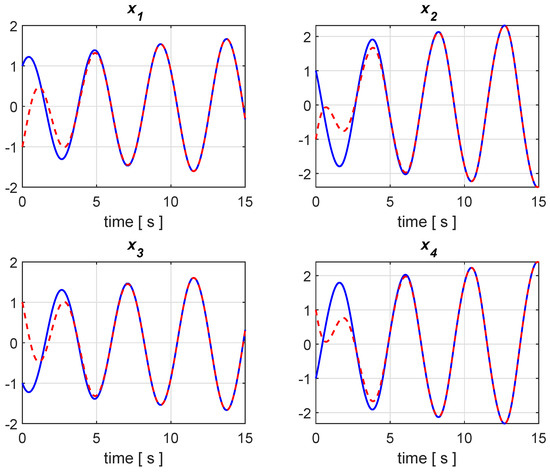
Figure 1. Simulation result without disturbances with states and estimated states in blue and red, respectively.

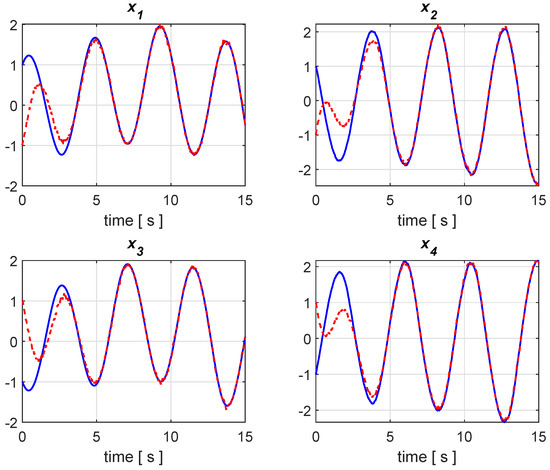
Figure 2. Simulation result with zero-mean, truncated Gaussian noises $w_i$ with variance equal to 1, $i=1,2,3,4$ with states and estimated states in blue and red, respectively.

4. Conclusions

In this paper, we have explored the use of ISS to investigate the stability of the estimations error provided by observers for system with Lipschitz non-linearities. This assumption turns out to be fundamental to bound the time derivative of Lyapunov functions and functionals from above. Thus, the extension to attack the same problem without the Lipschitz hypothesis seems to be nontrivial and needs to be replaced by other assumptions that allow to apply the proposed decomposition. In this respect, the adoption of metrics different from the Euclidean one [38,39,40] as well as of non-quadratic Lyapunov functions [41,42] may be the target of future investigations.

The proposed stability analysis has shown meaningful connections with the ISS theory (see, e.g., [43]), although some problems are still open. For example, an explicit evaluation of the sensitivity of the estimation error (i.e., the ISS gain of the disturbances) will be the target of future work. Another open question worth addressing is the converse of the sensitivity evaluation, i.e., the assignment of a desirable ISS gain by adopting a suitable observer structure.

References

- Thau, F.E. Observing the state of non-linear dynamic systems. Int. J. Control 1973, 17, 471–479. [Google Scholar] [CrossRef]
- Kou, S.R.; Elliott, D.L.; Tarn, T.J. Exponential observers for nonlinear dynamic systems. Inf. Control 1975, 29, 204–216. [Google Scholar] [CrossRef]
- Krener, A.J.; Isidori, A. Linearization by output injection and nonlinear observers. Syst. Control Lett. 1983, 3, 47–52. [Google Scholar] [CrossRef]
- Bestle, D.; Zeitz, M. Canonical form observer design for non-linear time-variable systems. Int. J. Control 1983, 38, 419–431. [Google Scholar] [CrossRef]
- Krener, A.J.; Respondek, W. Nonlinear observer with linearizable error dynamics. SIAM J. Control Optim. 1985, 23, 197–216. [Google Scholar] [CrossRef]
- Keller, H. Non-linear observer design by transformation into a generalized observer canonical form. Int. J. Control 1987, 46, 1915–1930. [Google Scholar] [CrossRef]
- Walcott, B.L.; Zak, S.H. State observation of nonlinear uncertain dynamical systems. IEEE Trans. Autom. Control 1987, 32, 166–170. [Google Scholar] [CrossRef]
- Slotine, J.J.; Hedrick, J.K.; Misawa, E.A. On sliding observers for nonlinear systems. J. Dyn. Syst. Meas. Control 1987, 109, 245–252. [Google Scholar] [CrossRef]
- Gauthier, J.P.; Hammouri, H.; Othman, S. A simple observer for nonlinear systems applications to bioreactors. IEEE Trans. Autom. Control 1992, 37, 875–880. [Google Scholar] [CrossRef]
- Gauthier, J.P.; Kupka, I.A.K. Observability and observers for nonlinear systems. SIAM J. Control Optim. 1994, 32, 975–994. [Google Scholar] [CrossRef]
- Astolfi, D.; Marconi, L. A high-gain nonlinear observer with limited gain power. IEEE Trans. Autom. Control 2015, 60, 3059–3064. [Google Scholar] [CrossRef]
- Zemouche, A.; Zhang, F.; Mazenc, F.; Rajamani, R. High-gain nonlinear observer with lower tuning parameter. IEEE Trans. Autom. Control 2019, 64, 3194–3209. [Google Scholar] [CrossRef]
- Khalil, H.; Praly, L. High-gain observers in nonlinear feedback control. Int. J. Robust Nonlinear Control 2014, 24, 993–1015. [Google Scholar] [CrossRef]
- Raghavan, S.; Hedrick, J.K. Observer design for a class of nonlinear systems. Int. J. Control 1994, 59, 515–528. [Google Scholar] [CrossRef]
- Rajamani, R. Observers for Lipschitz nonlinear nystems. IEEE Trans. Autom. Control 1998, 43, 397–401. [Google Scholar] [CrossRef]
- Hou, M.; Busawon, K.; Saif, M. Observer design based on triangular form generated by injective map. IEEE Trans. Autom. Control 2000, 45, 1350–1355. [Google Scholar] [CrossRef]
- Zemouche, A.; Boutayeb, M.; Bara, G. Observers for a class of Lipschitz systems with extension to H∞ performance analysis. Syst. Control Lett. 2008, 57, 18–27. [Google Scholar] [CrossRef]
- Sontag, E.D. The ISS philosophy as a unifying framework for stability-like behavior. In Lecture Notes in Control and Information Sciences; Isidori, A., Lamnabhi-Lagarrigue, F., Eds.; Springer Verlag: London, UK, 2000; pp. 443–467. [Google Scholar]
- Arcak, M.; Kokotovic, P. Nonlinear observer: A circle criterion design and robustness analysis. Automatica 2001, 37, 1923–1930. [Google Scholar] [CrossRef]
- Chaves, M.; Sontag, E. State-estimators for chemical reaction networks of Feinberg-Horn-Jackson zero deficiency type. Eur. J. Control 2002, 8, 343–359. [Google Scholar] [CrossRef]
- Shim, H.; Seo, J.H.; Teel, A.R. Nonlinear observer design via passivation of the error dynamics. Automatica 2003, 39, 885–892. [Google Scholar] [CrossRef]
- Alessandri, A. Observer design for nonlinear systems by using input-to-state stability. In Proceedings of the 43rd IEEE Conference on Decision and Control (CDC), Nassau, Bahamas, 14–17 December 2004; Volume 4, pp. 3892–3897. [Google Scholar]
- Alessandri, A.; Cervellera, C.; Macciò, D.; Sanguineti, M. Optimization based on quasi-Monte Carlo sampling to design state estimators for nonlinear systems. Optimization 2010, 59, 963–984. [Google Scholar] [CrossRef]
- Boyd, S.; El Ghaoui, L.; Feron, E.; Balakrishnan, V. Linear Matrix Inequalities in System and Control Theory; Studies in Applied Mathematics; SIAM: Philadelphia, PA, USA, 1994; Volume 15. [Google Scholar]
- Alessandri, A. On Hamilton-Jacobi approaches to state reconstruction for dynamic systems. Adv. Math. Phys. 2020, 2020, 9643291. [Google Scholar] [CrossRef]
- Alessandri, A. Lyapunov functions for state observers of dynamic systems using Hamilton-Jacobi inequalities. Mathematics 2020, 8, 202. [Google Scholar] [CrossRef]
- Alessandri, A. Sliding-mode estimators for a class of nonlinear systems affected by bounded disturbances. Int. J. Control 2002, 76, 226–236. [Google Scholar] [CrossRef]
- Alessandri, A. Design of observers for Lipschitz nonlinear systems using LMI. IFAC Proc. Vol. 2004, 37, 459–464. [Google Scholar] [CrossRef]
- Shim, H.; Son, Y.I.; Seo, J.H. Semi-global observer for multi-output nonlinear systems. Syst. Control Lett. 2001, 42, 233–244. [Google Scholar] [CrossRef]
- Sontag, E.D. Smooth stabilization implies coprime factorization. IEEE Trans. Autom. Control 1989, 34, 435–443. [Google Scholar] [CrossRef]
- Sontag, E.D. Remarks on stabilization and input-to-state stability. In Proceedings of the 28th Conference on Decision and Control, Tampa, FL, USA, 13–15 December 1989; pp. 1376–1378. [Google Scholar]
- Sontag, E.D. A remark on the converging-input converging-state property. IEEE Trans. Autom. Control 2003, 48, 313–314. [Google Scholar] [CrossRef]
- Khalil, H.K. Nonlinear Systems; Prentice Hall: Upper Saddle River, NJ, USA, 1995. [Google Scholar]
- Sontag, E.D.; Wang, Y. On characterizations of input-to-state stability property. Syst. Control Lett. 1995, 24, 351–359. [Google Scholar] [CrossRef]
- Sontag, E.D.; Teel, A. Changing supply functions in input/state stable systems. IEEE Trans. Autom. Control 1995, 40, 1476–1478. [Google Scholar] [CrossRef]
- Sontag, E.D. New characterization of input-to-state stability. IEEE Trans. Autom. Control 1996, 41, 1283–1294. [Google Scholar] [CrossRef]
- Löfberg, J. YALMIP: A toolbox for modeling and optimization in MATLAB. In Proceedings of the CACSD Conference, New Orleans, LA, USA, 2–4 September 2004; pp. 284–289. [Google Scholar]
- Manojlović, V. On conformally invariant extremal problems. Appl. Anal. Discret. Math. 2009, 3, 97–119. [Google Scholar] [CrossRef][Green Version]
- Todorčević, V. Harmonic Quasiconformal Mappings and Hyperbolic Type Metrics; Springer International Publishing: Cham, Switzerland, 2019. [Google Scholar]
- Ciric, L. Some Recent results in Metrical Fixed Point Theory; Technical Report; University of Belgrade: Beograd, Serbia, 2003. [Google Scholar]
- Hosseinzadeh, M.; Yazdanpanah, M. Performance enhanced model reference adaptive control through switching non-quadratic Lyapunov functions. Syst. Control Lett. 2015, 76, 47–55. [Google Scholar] [CrossRef]
- Lu, C.; Hua, L.; Zhang, X.; Wang, H.; Guo, Y. Adaptive sliding mode control method for Z-axis vibrating gyroscope using prescribed performance approach. Appl. Sci. 2020, 10, 4779. [Google Scholar] [CrossRef]
- Angeli, D. A Lyapunov approach to incremental stability. IEEE Trans. Autom. Control 2002, 47, 410–421. [Google Scholar] [CrossRef]
© 2020 by the authors. Licensee MDPI, Basel, Switzerland. This article is an open access article distributed under the terms and conditions of the Creative Commons Attribution (CC BY) license (http://creativecommons.org/licenses/by/4.0/).