Similarity Measures for Learning in Lattice Based Biomimetic Neural Networks

Abstract

This paper presents a novel lattice based biomimetic neural network trained by means of a similarity measure derived from a lattice positive valuation. For a wide class of pattern recognition problems, the proposed artificial neural network, implemented as a dendritic hetero-associative memory delivers high percentages of successful classification. The memory is a feedforward dendritic network whose arithmetical operations are based on lattice algebra and can be applied to real multivalued inputs. In this approach, the realization of recognition tasks, shows the inherent capability of prototype-class pattern associations in a fast and straightforward manner without need of any iterative scheme subject to issues about convergence. Using an artificially designed data set we show how the proposed trained neural net classifies a test input pattern. Application to a few typical real-world data sets illustrate the overall network classification performance using different training and testing sample subsets generated randomly.

1. Introduction

The lattice neural network discussed in this paper is a biomimetic neural network. The term biomimetic refers to man-made systems of processes that imitate nature. Accordingly, biomimetic artificial neurons are man-made models of biological neurons, while biomimetic computational systems deal mostly with information processing in the brain. More specifically, biomimetic computational systems are concerned with such questions as how do neurons encode, transform and transfer information, and how this encoding and transfer of information can be expressed mathematically.

In the human as well as other mammal brains, every neuron has a cell body, named soma, and two kinds of physiological processes called, respectively, dendrites and axons [1]. Multiple dendrites conduct electric impulses toward the body of the cell whereas the axon conducts signals from the soma. Usually, dendrites have many branches forming complicated large trees and various types of dendrites are studded with many tiny branches known as spines. When present, dendrite spines are the main postsynaptic target for synaptic input. The input surface of the neuron is composed of the cell body and the dendrites. Those neurons receiving a firing signal coming from a presynaptic neuron are called postsynaptic neurons.

The axon hillock, usually located in the opposite pole of a neural cell, gives rise to the axon which is a long fiber whose branches form the axonal tree or arborization. In some neurons, besides its terminal arborization, the axon may have branches at intervals along its length. In general, a branch of an axon ends in several tips, called nerve terminals, synaptic knobs or boutons, and the axon, being the main fiber branch of a neuron, carries electric signals to other neurons. An impulse traveling along an axon from the axon hillock propagates all the way through the axonal tree to the nerve terminals. The boutons of the branches make contact at synaptic sites of the cell body and the many dendrites of other neurons. The synapse is a specialized structure whereby neurons communicate without actual physical contact between the two neurons at the synaptic site. The synaptic knob is separated from the surface of the soma or dendrite by a very short space known as the synaptic cleft. The mechanism characteristics of a synaptic structure are basically well known and there are two types of synapses, inhibitory synapses that prevent the neuron from firing impulses in response to excitatory synapses, which tend to depolarize the postsynaptic membrane and consequently exciting the postsynaptic cell to fire impulses.

In the cerebral cortex, the majority of synapses take place in the neural dendritic trees and much of the information processing is realized by the dendrites as brain studies have revealed [2,3,4,5,6,7,8]. A human brain has around 85 billion neurons and the average number of synaptic connections a neuron may have with other nearby neurons is about $7,000$ [9,10,11,12]. More specifically, a single neuron in the cerebral cortex has a number of synapses within the range 500 to $200,000$, and an adult’s cerebral cortex has an estimated number of synapses in the range of 100 to 500 trillion (${10}^{14}$ to $5\times {10}^{14}$) [10,13,14,15]. In both volume and surface area of the brain, dendrites make up the largest component spanning all cortical layers in every region of the cerebral cortex [2,4,16]. Thus, in order to model an artificial neural network that can represent more faithfully a biological brain network, it is not possible to ignore dendrites and their spines, which cover the membrane of a neuron in more than $50\%$. This is particularly true by considering that several brain researchers have proposed that dendrites (not the neuron) are the basic computing devices of the brain. Neurons together with its associated dendritic structure can work as multiple, almost independent, functional subunits where each subunit can implement different logical operations [3,4,16,17,18,19]. The interested reader may peruse the works of some researchers [3,4,5,6,7,8,16,20,21], that have proposed possible biophysical mechanisms for dendritic computation of logical functions such as ‘AND’, ‘NOT’, ‘OR’, and ‘XOR’.

It is in light of these observations that we modeled biomimetic artificial neural networks based on dendritic computing. The binary logic operations ‘AND’ and ‘OR’ are naturally extended to non-binary numbers by considering their arithmetical equivalence, respectively, with finding the minimum and maximum of two numbers. Thus, the logic unary operation ‘NOT’, min and max together with addition belong to the class of machine operations that contribute to the high speed performance of digital computers. The preceding fact suggests us to select as the principal computational foundation, the algebraic structure provided by the bounded lattice ordered group $({\mathbb{R}}_{\pm \infty }^n,\vee ,\wedge ,+,{+}^{*})$ [22,23,24]. Recall that, ${\mathbb{R}}_{\pm \infty }$ stands for the set of extended real numbers and the binary operations of maximum, minimum, and extended additions are denoted, respectively, by ∨, ∧, and $+/{+}^{*}$.

The core issue in this research is a novel method for learning in biomimetic lattice neural networks. However, currently biomimetic neural networks and lattice based computational intelligence are not part of mainstream artificial neural networks (ANNs) and artificial intelligence (AI). To acquaint readers that are unfamiliar with these topics, we organized this paper as follows: Section 2 deals with basic concepts from lattice theory that are essential conceptual background, while Section 3 provides a short introduction to lattice biomimetic neural networks. Section 4 discusses the construction of the biomimetic neural network during the learning stages, and the illustrative examples provided in Section 5 show that the proposed neural architecture based on lattice similarity measures can be trained to give high percentages of correct classification in multiclass real-world pattern recognition datasets. The paper ends with Section 6, where we give our conclusions and some relevant comments.

2. Lattice Theory Background Material

Lattice theory is based on the concept of partially ordered sets, while partially ordered sets rest on the notion of binary relations. More specifically, given a set X and $R\subset X\times X=\left\{\right(x,y):x,y\in X\}$, then R is called a binary relation on X. For example, set inclusion is a relation on any power set $\mathcal{P}\left(X\right)$ of a set X. In particular, if X is a set and $S=\left\{\right(A,B):A\subset B$ with $A,B\in \mathcal{P}\left(X\right)\}$, then S is a binary relation on $\mathcal{P}\left(X\right)$. Note that this example shows that a pair of elements of $\mathcal{P}\left(X\right)$ need not be a member pair of the binary relation. In contrast, the relation of less or equal, denoted by ≤, between real numbers is the set $\left\{\right(x,y):x\le y\}\subset \mathbb{R}\times \mathbb{R}$. Here, each pair of elements of $\mathbb{R}$ is related. The two examples of a binary relation on a set belong to a special case of binary relations known as partial order relations. We shall use the symbol ≼ for denoting a binary relation on an unspecified set X.

Definition 1.

A relation ≼ on a set P is called a partial order on P if and only if for every $x,y,z\in P$, the following three conditions are satisfied:

• $x\preccurlyeq x$ (reflexivity),
• $x\preccurlyeq y$ and $y\preccurlyeq x$⇒$x=y$ (antisymmetry) and
• $x\preccurlyeq y$ and $y\preccurlyeq z$⇒$x\preccurlyeq z$ (transitivity).

A set P together with a partial order ≼, denoted by $(P,\preccurlyeq )$, is called a partially ordered set or simply a poset. If $x\preccurlyeq y$ in a partially ordered set, then we say that x precedes y or that x is included in y and that y follows x or that y includes x. If $(P,\preccurlyeq )$ is a poset, then we define the notation $x\prec y$, where $x,y\in P$, to mean that $x\preccurlyeq y$ and $x\ne y$. The following theorem is a trivial consequence of these definitions.

Theorem 1.

Suppose $(P,\preccurlyeq )$ is a poset. Consequently,

• If $Q\subset P$, then $(Q,\preccurlyeq )$ is also a poset,
• $\nexists x\in P\ni x\prec x$, and
• if $x\prec y$ and $y\prec z$, then $x\prec z$, where $x,y,z\in P$.

If X is a set, then for any pair $C,D\in \mathcal{P}\left(X\right)$ the set $\{C,D\}$ has a least upper bound and a greatest lower bound, namely $C\cup D$ and $C\cap D$, respectively. Thus, $(C\cap D,C\cup D)\in \left\{\right(A,B):A\subset B$ with $A,B\in \mathcal{P}\left(X\right)\}$. The greatest lower bound and least upper bound of a subset are commonly denoted by glb$\{C,D\}$ and lub$\{C,D\}$, respectively. Similarly, if $\mathbf{x},\mathbf{y}\in {\mathbb{R}}^n$, then lub$\{\mathbf{x},\mathbf{y}\}=\mathbf{x}\vee \mathbf{y}$ and glb$\{\mathbf{x},\mathbf{y}\}=\mathbf{x}\wedge \mathbf{y}$, so that $(\mathbf{x}\wedge \mathbf{y},\mathbf{x}\vee \mathbf{y})\in \left\{\right(\mathbf{p},\mathbf{q}):\mathbf{p}\le \mathbf{q}$ and $\mathbf{p},\mathbf{q}\in {\mathbb{R}}^n\}$. The notions of least upper bound and greatest lower bound are key in defining the concept of a lattice.

More generally, if P is a poset and $X\subset P$, then the infimum denoted by $inf\left(X\right)$, if it exist, is the greatest element in P that is less than or equal to all elements of X. Likewise, the supremum written as $sup\left(X\right)$, if it exists, is the least element in P that is greater than or equal to all elements of X. Consequently, the infimum and supremum correspond, respectively, to the greatest lower bound and the least upper bound.

A few fundamental types of posets are described next: (1) A lattice is a partially ordered set L such that for any two elements $x,y\in L$, $inf\{x,y\}$ and $sup\{x,y\}$ exist. If L is a lattice, then we denote $inf\{x,y\}$ by $x\wedge y$ and $sup\{x,y\}$ by $x\vee y$, respectively. The expression $x\wedge y$ is also referred to as the meet or min of x and y, while $x\vee y$ is referred to as the join or max of x and y. (2) A sublattice of a lattice L is a subset X of L such that for each pair $x,y\in X$, we have that $x\wedge y\in X$ and $x\vee y\in X$. (3) A lattice L is said to be complete if and only if for each of its subsets X, $inf\left(X\right)$ and $sup\left(X\right)$ exist. The symbols $\bigwedge X$ and $\bigvee X$ are also commonly used for $inf\left(X\right)$ and $sup\left(X\right)$, respectively.

Suppose L is a lattice and also an additive Abelian group, which we denote by $(L,+)$. Now, consider the function $\phi :L\to L$ defined by $\phi \left(x\right)=-x$. If $x\preccurlyeq y$, then $\phi (x\vee y)=-(x\vee y)=-y$ and $\phi \left(x\right)\wedge \phi \left(y\right)=-x\wedge -y=-y$ since $-y\preccurlyeq -x$. Likewise, if $y\preccurlyeq x$, then $\phi (x\vee y)=-x$ and $\phi \left(x\right)\wedge \phi \left(y\right)=-x$. Therefore, $\phi (x\vee y)=\phi \left(x\right)\wedge \phi \left(y\right)$. Similarly, $\phi (x\wedge y)=\phi \left(x\right)\vee \phi \left(y\right)$. This verifies the dual equations:

$$\begin{array}{cc}\hfill -(a\vee b)=-a\wedge -b& \mathrm{and}a\vee b=-(-a\wedge -b),\hfill \end{array}$$

(1)

$$\begin{array}{cc}\hfill -(a\wedge b)=-a\vee -b& \mathrm{and}a\wedge b=-(-a\vee -b),\hfill \end{array}$$

(2)

signifying that the function $\psi \left(x\right)=a+(-x)+b$ is a dual isomorphism for any fixed pair $a,b\in L$. Thus, in any lattice Abelian group the following identities hold:

$$\begin{array}{cc}\hfill a+-(x\vee y)+b& =(a-x+b)\wedge (a-y+b),\hfill \end{array}$$

(3)

$$\begin{array}{cc}\hfill a+-(x\wedge y)+b& =(a-x+b)\vee (a-y+b).\hfill \end{array}$$

(4)

These equations easily generalize to,

$$a+(-\underset{i=1}{\overset{n}{\bigvee }}{x}_i)+b=\underset{i=1}{\overset{n}{\bigwedge }}(a-x_i+b)\mathrm{and}a+(-\underset{i=1}{\overset{n}{\bigwedge }}{x}_i)+b=\underset{i=1}{\overset{n}{\bigvee }}(a-x_i+b),$$

(5)

hence, if $b=0$, then,

$$a+\left(-\underset{i=1}{\overset{n}{\bigvee }}{x}_i\right)=\underset{i=1}{\overset{n}{\bigwedge }}(a-x_i)\mathrm{and}a+\left(-\underset{i=1}{\overset{n}{\bigwedge }}{x}_i\right)=\underset{i=1}{\overset{n}{\bigvee }}(a-x_i).$$

(6)

Some of the most useful computational tools for applications of lattice theory to real data sets are mappings of lattices to the real number system. One family of such mappings are valuation functions.

Definition 2.

A valuation on a lattice L is a function $v:L\to \mathbb{R}$ that satisfies:

$$v\left(x\right)+v\left(y\right)=v(x\vee y)+v(x\wedge y)\forall x,y\in L.$$

(7)

A valuation is said to be isotone if and only if $x\preccurlyeq y\Rightarrow v\left(x\right)\le v\left(y\right)$ and positive if and only if $x\prec y\Rightarrow v\left(x\right)<v\left(y\right)$.

The importance of valuations on lattices is due to their close association with various measures. Among these measures are pseudometrics and metrics.

Theorem 2.

If L is a lattice and v is an isotone valuation on L, then the function $d:L\times L\to \mathbb{R}$ defined by:

$$d(x,y)=v(x\vee y)-v(x\wedge y),$$

(8)

satisfies, $\forall x,y,z,a\in L$, the following conditions:

• $d(x,y)\ge 0$ and $d(x,x)=0$,
• $d(x,y)=d(y,x)$,
• $d(x,y)\le d(x,z)+d(z,y)$, and
• $d(x,y)\ge d(a\vee x,a\vee y)+d(a\wedge x,a\wedge y)$.

An elegant proof of this theorem is provided by Birkhoff in [25]. In fact, the condition:

$$x\wedge y\prec x\vee y\iff v(x\wedge y)\prec v(x\vee y),$$

(9)

or equivalently, $d(x,y)=0\iff x=y$, yields the following corollary of Theorem 2.

Corollary 1.

Suppose L is a lattice and v is an isotone valuation on L. The function $d(x,y)=v(x\vee y)-v(x\wedge y)$ is a metric on L if and only if the valuation v is positive.

The metric d defined on a lattice L in terms of an isotone positive valuation is called a lattice metric or simply an ℓ-metric, and the pair $(L,d)$ is called a metric lattice or a metric lattice space. The importance of ℓ-metrics is due to the fact that they can be computed using only the operations of ∨, ∧, and + for lattices that are additive Abelian groups. For the lattice group $({\mathbb{R}}^n,+)$, they require far less computational time than any ${\ell }_p$ metric whenever $1<p<\infty$. Just as different ${\ell }_p$ norms give rise to different ${\ell }_p$ metrics on ${\mathbb{R}}^n$, different positive valuations on a lattice will yield different ℓ-metrics. For instance, if $L={\mathbb{R}}^n$, then the two positive valuations $v_1\left(\mathbf{x}\right)={\sum }_{i=1}^n{x}_i$ and $v_{\infty }\left(\mathbf{x}\right)={\bigvee }_{i=1}^n{x}_i$ define two different ℓ-metrics on L. In particular, we have:

Theorem 3.

For $\mathbf{x},\mathbf{y}\in L$, the induce metrics $d_1$ and $d_{\infty }$ on $L\times L$ are given by,

$$d_1(\mathbf{x},\mathbf{y})=v_1(\mathbf{x}\vee \mathbf{y})-v_1(\mathbf{x}\wedge \mathbf{y})and{d}_{\infty }(\mathbf{x},\mathbf{y})=v_{\infty }(\mathbf{x}\vee \mathbf{y})-v_{\infty }(\mathbf{x}\wedge \mathbf{y}).$$

(10)

Proof. 

Considering (1) through (4) establishes the following equalities:

$$\begin{array}{cc}\hfill v_1(\mathbf{x}\vee \mathbf{y})-v_1(\mathbf{x}\wedge \mathbf{y})& =\sum _{i=1}^n(x_i\vee y_i)-\sum _{i=1}^n(x_i\wedge y_i)=\sum _{i=1}^n[(x_i\vee y_i)-(x_i\wedge y_i)]\hfill \\ \hfill & =\sum _{i=1}^n[(x_i\vee y_i)-x_i]\vee [(x_i\vee y_i)-y_i]\hfill \\ \hfill & =\sum _{i=1}^n[(x_i-x_i)\vee (y_i-x_i)]\vee [(x_i-y_i)\vee (y_i-y_i)]\hfill \\ \hfill & =\sum _{i=1}^n(y_i-x_i)\vee (x_i-y_i)=\sum _{i=1}^n|x_i-y_i|=d_1(\mathbf{x},\mathbf{y}).\hfill \end{array}$$

Replacing the sum ∑ by the maximum operation ⋁ and using an analogous argument proves the second equality in (10) of the theorem. □

In addition to ℓ-metrics, valuations also give rise to similarity measures. A similarity measure is a measure that for a given object x tries to decide how similar or dissimilar other objects are when compared to x. For objects represented by vectors, distance measures such as metrics, measure numerically how unlike or different two data points are, while similarity measures find numerically how alike two data points are. In short, a similarity measure is the antithesis of a distance measure since a higher value indicates a greater similarity, while for a distance measure a lower value indicates greater similarity. There exists an assortment of different similarity measures, depending on the sets, spaces, or lattices under consideration. Specifically, for lattices we have the following,

Definition 3.

If L is a lattice with $inf\left(L\right)=O$, then a similarity measure for $y\in L$ is a mapping $s:L\times L\to [0,1]$ defined by the following conditions:

• $s(x,O)=0,\forall x\ne O$,
• $s(x,x)=1,\forall x\in L$, and
• $s(x,y)<1,\forall x\ne y$.

The basic idea is that if $y\in L$ has more features in common with z than any other $x\in L$ or if y is closer to z than any other $x\in L$ in some meaningful way, then $s(x,z)<s(y,z)$. As an aside, there is a close relationship of similarity measures with fuzzy sets. Specifically, if $X=L\times L$, then $F=\left\{\right((x,y),s(x,y)):(x,y)\in X\}$ is a fuzzy set with membership function $s:X\to [0,1]$.

3. Lattice Biomimetic Neural Networks

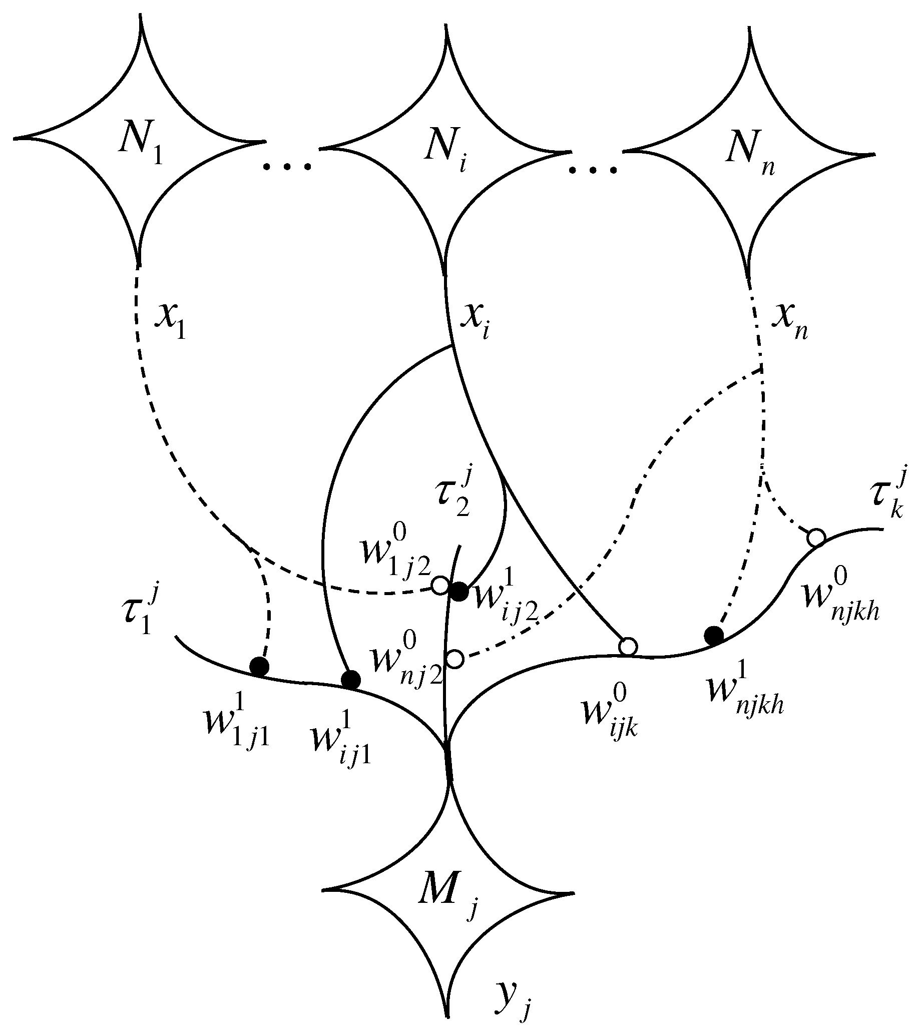
In ANNs endowed with dendrites whose computation is based on lattice algebra, a set $N_1,\dots ,N_n$ of presynaptic neurons provides information through its axonal arborization to the dendritic trees of some other set $M_1,\dots ,M_m$ of postsynaptic neurons [26,27,28]. Figure 1 illustrates the neural axons and branches that go from the presynaptic neurons to the postsynaptic neuron $M_j$, whose dendritic tree has $K_j$ branches, denoted by, ${\tau }_1^j,\dots ,{\tau }_{K_j}^j$ and containing the synaptic sites upon which the axonal fibers of the presynaptic neurons terminate. The address or location of a specific synapse is defined by the quintuple $(i,j,k,h,\ell )$, where $i\in \{1,\dots ,n\}$, $j\in \{1,\dots ,m\}$, and $k\in \{1,\dots ,K_j\}$, that a terminal axonal branch of $N_i$ has a bouton on the k-th dendritic branch ${\tau }_k^j$ of $M_j$. The index $h\in \{1,\dots ,\rho \}$ denotes the h-th synapse of $N_i$ on ${\tau }_k^j$ since there may be more terminal axonal branches of $N_i$ synapsing on ${\tau }_k^j$. The index $\ell \in \{0,1\}$ classifies the type of the synapse, where $\ell =0$ indicates that the synapse at $(i,j,k,h,\ell )$ is inhibitory (i.e., releases inhibitory neurotransmitters) and $\ell =1$ indicates that the synapse is excitatory (releases excitatory neurotransmitters).

The strength of the synapse $(i,j,k,h,\ell )$ corresponds to a real number, commonly referred to as the synaptic weight and customarily denoted by $w_{ijkh}^{\ell }$. Thus, if S denotes the set of synapses on the dendritic branches of the set of the postsynaptic neurons $M_1,\dots ,M_m$, then w can be viewed as the function, $w:S\to \mathbb{R}$, defined by $w(i,j,k,h,\ell )=w_{ijkh}^{\ell }$ where $w_{ijkh}^{\ell }\in \mathbb{R}$. In order to reduce notational overhead we simplify the synapse location and type as follows:

• $(j,k,h,\ell )$ if $n=1$ and set $N=N_1$ (single input neuron),
• $(i,k,h,\ell )$ if $m=1$, set $M=M_1$ (single output neuron) and denote its dendritic branches by ${\tau }^1,\dots ,{\tau }^K$ (multiple dendrites) or simply $\tau$ if $K=1$ (single dendrite), and
• $(i,j,k,\ell )$ if $\rho =1$ (at most one synapse per dendrite).

The axon terminals of different presynaptic biological neurons that have synaptic sites on a single branch of the dendritic tree of a postsynaptic neuron may release dissimilar neurotransmitters, which, in turn, affect the receptors of the branch. Since the receptors serve as storage sites of the synaptic strengths, the resulting electrical signal generated by the branch is the result of the combination of the output of all its receptors. As the signal travels toward the cell’s body it again combines with signals generated in the other branches of the dendritic tree. In the lattice based biomimetic model, the various biological synaptic processes due to dissimilar neurotransmitters are replaced by different operations of a lattice group. More specifically, if $\Omega =\{\vee ,\wedge ,+\}$ represents the operations of a lattice group G, then the generic symbols ⊕, ⊗, and ⊙ will mean that $\oplus ,\otimes ,\odot \in \Omega$, but are not explicitly specified numerical operations. For instance, if ${⨁}_{i=1}^n{a}_i=a_1\oplus \cdots \oplus a_n$ and $\oplus =\vee$, then ${⨁}_{i=1}^n{a}_i={\bigvee }_{i=1}^n{a}_i=a_1\vee \cdots \vee a_n$, and if $\oplus =+$, then ${⨁}_{i=1}^n{a}_i={\sum }_{i=1}^n{a}_i=a_1+\cdots +a_n$.

Let $\mathbf{x}=(x_1,\cdots ,x_n)\in G^n$ and let $p_{jk}$ be the switching value that signals the final outflow from the k-th branch reaching $M_j$; if excitatory, then $p_{jk}=1$ or if inhibitory then $p_{jk}=-1$. Also, let $I\left(k\right)\subseteq \{1,\cdots ,n\}$ represent the index set corresponding to all presynaptic neurons with terminal axonal fibers that synapse on the k-th dendrite of $M_j$, and let $\rho$ be the number of synaptic knobs of $N_i$ contacting branch $d_{jk}$. Therefore, if $N_i$ sends the information value $x_i\in G$ via its axon and attached branches, the total output (or response) of a branch ${\tau }_k^j$ to the received input at its synaptic sites is given by the general formula:

$${\tau }_k^j\left(\mathbf{x}\right)=p_{jk}\underset{i\in I\left(k\right)}{⨁}\underset{h=1}{\overset{\rho }{⨂}}{(-1)}^{1-\ell }(x_i\odot w_{ijkh}^{\ell }),$$

(11)

The cell body of $M_j$ receives ${\tau }_k^j\left(\mathbf{x}\right)$, and its state is a function of the combined values processed by its dendritic structure. Hence, the state of $M_j$ is computed as,

$${\tau }^j\left(\mathbf{x}\right)=p_j\underset{k=1}{\overset{K_j}{⨀}}{\tau }_k^j\left(\mathbf{x}\right),$$

(12)

where $p_j=\pm 1$ denotes the response of the cell to the received input. As explained before, $p_j=1$ (excitation) means acceptance of the received input and $p_j=-1$ (inhibition) means rejection. This mimics the summation that occurs in the axonal hillock of biological neurons. In many applications of lattice neural networks (LNNs), the presynaptic neurons have at most one axonal bouton synapsing ($\rho =1$) on any given dendritic branch ${\tau }_k^j$. In these cases, (11) simplifies to,

$${\tau }_k^j\left(\mathbf{x}\right)=p_{jk}\underset{i\in I\left(k\right)}{⨁}{(-1)}^{1-\ell }(x_i\odot w_{ijk}^{\ell }).$$

(13)

As in most ANNs, the next state of $M_j$ is determined by an activation function $f_j$, which—depending on the problem domain—can be the identity function, a simple hard limiter, or a more complex function. The next state refers to the information being transferred via $M_j$’s axon to the next level neurons or the output if $M_j$ is an output neuron. Any ANN that is based on dendritic computing and employs equations of type (11) and (12), or (13) and (12), will be called a lattice biomimetic neural network (LBNN). In the technical literature, there exist a multitude of different models of lattice based neural networks. The matrix based lattice associative memories (LAMs) discussed in [22,24,29,30] and LBNNs are just a few examples of LNNs. What sets LBNNs apart from current ANNs are the inclusion of the following processes employed by biological neurons:

• The use of dendrites and their synapses.
• A presynaptic neuron $N_i$ can have more than one terminal branch on the dendrites of a postsynaptic neuron $M_j$.
• If the axon of a presynaptic neuron $N_i$ has two or more terminal branches that synapse on different dendritic locations of the postsynaptic neuron $M_j$, then it is possible that some of the synapses are excitatory and others are inhibitory to the same information received from $N_i$.
• The basic computations resulting from the information received from the presynaptic neurons takes place in the dendritic tree of $M_j$.
• As in standard ANNs, the number of input and output neurons is problem dependent. However, in contrast to standard ANNs where the number of neurons in a hidden layer, as well as the number of hidden layers are pre-set by the user or an optimization process, hidden layer neurons, dendrites, synaptic sites and weights, and axonal structures are grown during the learning process.

Substituting specific lattice operations in the general Equations (11) and (12) results in a specific model of the computations performed by the postsynaptic neuron $M_j$. For instance, two distinct specific models are given by,

$${\tau }_k^j\left(\mathbf{x}\right)=p_{jk}\sum _{i\in I\left(k\right)}\left[\underset{h=1}{\overset{\rho }{\bigwedge }}{(-1)}^{1-\ell }(x_i+w_{ijkh}^{\ell })\right]\mathrm{and}{\tau }^j\left(\mathbf{x}\right)=p_j\underset{k=1}{\overset{K_j}{\bigvee }}{\tau }_k^j\left(\mathbf{x}\right),$$

(14)

or,

$${\tau }_k^j\left(\mathbf{x}\right)=p_{jk}\underset{i\in I\left(k\right)}{\bigwedge }\left[\underset{h=1}{\overset{\rho }{\bigwedge }}{(-1)}^{1-\ell }(x_i+w_{ijk}^{\ell })\right]\mathrm{and}{\tau }^j\left(\mathbf{x}\right)=p_j\underset{k=1}{\overset{K_j}{\bigvee }}{\tau }_k^j\left(\mathbf{x}\right).$$

(15)

Unless otherwise mentioned, the lattice group $(\mathbb{R},\wedge ,\vee ,+)$ will be employed when implementing Equations (11) and (12) or (13) and (12). In contrast to standard ANNs currently in vogue, we allow both negative and positive synaptic weights as well as weights of value zero. The reason for this is that these values correspond to positive weights if one chooses the algebraically equivalent lattice group $({\mathbb{R}}^{+},\wedge ,\vee ,\times )$, where ${\mathbb{R}}^{+}=\{x\in \mathbb{R}:x>0\}$. The equivalence is given by the bijection $f:\mathbb{R}\to {\mathbb{R}}^{+}$, which is defined by $f\left(x\right)=exp\left(x\right)$. Consequently, negative weights correspond to small positive weights and zero weights to one.

4. Similarity Measure Based Learning for LBNNs

The focus of this section is on the pattern recognition capabilities of LBNNs. In particular, on how a lattice biomimetic neural network learns to recognize distinct patterns. However, since the learning method presented here is based on a specific similarity measure, we begin our discussion by describing the measure used [31]. The lattice of interest in our discussion is $L={\mathbb{R}}^{*}=\{\mathbf{x}\in {\mathbb{R}}^n:\mathbf{x}\ge \mathbf{0}$, with $inf\left(L\right)=\mathbf{0}$, while the similarity measure for $\mathbf{y}\in L$ is the mapping $s:L\times L\to [0,1]$ defined by:

$$s(\mathbf{x},\mathbf{y})=\frac{v\left(\mathbf{y}\right)}{v(\mathbf{x}\vee \mathbf{y})}\wedge \frac{v(\mathbf{x}\wedge \mathbf{y})}{v\left(\mathbf{y}\right)},$$

(16)

where v is the isotone positive lattice valuation given by $v\left(\mathbf{x}\right)={\sum }_{i=1}^n{x}_i$. We used the lattice $L=({\mathbb{R}}^{*},\vee ,\wedge )$ in order to satisfy Condition (1) of Definition 3, and coordinates of pattern vectors considered here are nonnegative. Since data sets are finite, data sets consisting of pattern vectors that are subsets of ${\mathbb{R}}^n$ have always an infimum $\mathbf{v}$ and a supremum $\mathbf{u}$. Thus, if $Q\subset {\mathbb{R}}^n$ is a dataset whose pattern vectors have both negative and nonnegative coordinates, simply compute $\mathbf{v}={\bigwedge }_{\mathbf{q}\in Q}\mathbf{q}=inf\left(Q\right)$ and $\mathbf{u}={\bigvee }_{\mathbf{q}\in Q}\mathbf{q}=sup\left(Q\right)$. Note that the hyperbox $L_Q=[\mathbf{v},\mathbf{u}]=\{\mathbf{x}\in {\mathbb{R}}^n:v_i\le x_i\le u_i;i=1,\dots ,n\}$ is a complete lattice and $Q\subset L_Q$. Setting ${\mathbf{x}}^{\prime }=\mathbf{x}-\mathbf{v}$, then ${\mathbf{v}}^{\prime }=\mathbf{0}$ and ${\mathbf{x}}^{\prime }\in {\mathbb{R}}^{*},\forall \mathbf{x}\in L_Q$. Finally, define the mapping $s^{\prime }:L_Q\to [0,1]$ by setting $s^{\prime }(\mathbf{x},\mathbf{y})=s({\mathbf{x}}^{\prime },{\mathbf{y}}^{\prime })$ where ${\mathbf{x}}^{\prime }=\mathbf{x}-\mathbf{v}$ and ${\mathbf{y}}^{\prime }=\mathbf{y}-\mathbf{v}$. It follows that $s^{\prime }(\mathbf{x},\mathbf{v})=s({\mathbf{x}}^{\prime },{\mathbf{v}}^{\prime })=s(\mathbf{x}-\mathbf{v},\mathbf{0})=0$, which proves that Condition (1) of Definition 3 is satisfied, and the remaining two conditions are similarly proven.

There exist several distinct methods for learning in LBNNs. The method described here is novel in that it is based on the similarity measure given in (16). To begin with, suppose $Q=\{{\mathbf{q}}^1,\dots ,{\mathbf{q}}^k\}\subset {\mathbb{R}}^n$ is a data set consisting of prototype patterns, where each pattern ${\mathbf{q}}^j$ belongs to one of m different classes. Here $1<m<k$ and we use the expression ${\mathbf{q}}^j\in c_{\lambda }$ if ${\mathbf{q}}^j$ belongs to class $\lambda \in \{1,\dots ,m\}$ by some predefined relationship. Letting ${\mathbb{N}}_m=\{1,\dots ,m\}$, then the association of patterns and their class membership is a subset of $Q\times {\mathbb{N}}_m$ specified by $H=\{({\mathbf{q}}^j,c_{\lambda }):{\mathbf{q}}^j\in Q,\lambda \in {\mathbb{N}}_m\}$.

As in most learning methods for artificial neural networks, a lattice biomimetic neural network learns to recognize distinct patterns by using a subset of prototype patterns stored in a hetero-associative memory. Given the data set Q, learning in LBNNs begins with selecting a family of prototypes $P_p=\{{\mathbf{q}}^{s_1},\dots ,{\mathbf{q}}^{s_{\eta }}\}\subset Q$. The selection is random and the subscript p is a predefined percentage $p\%$ of the total number of the k samples in Q.

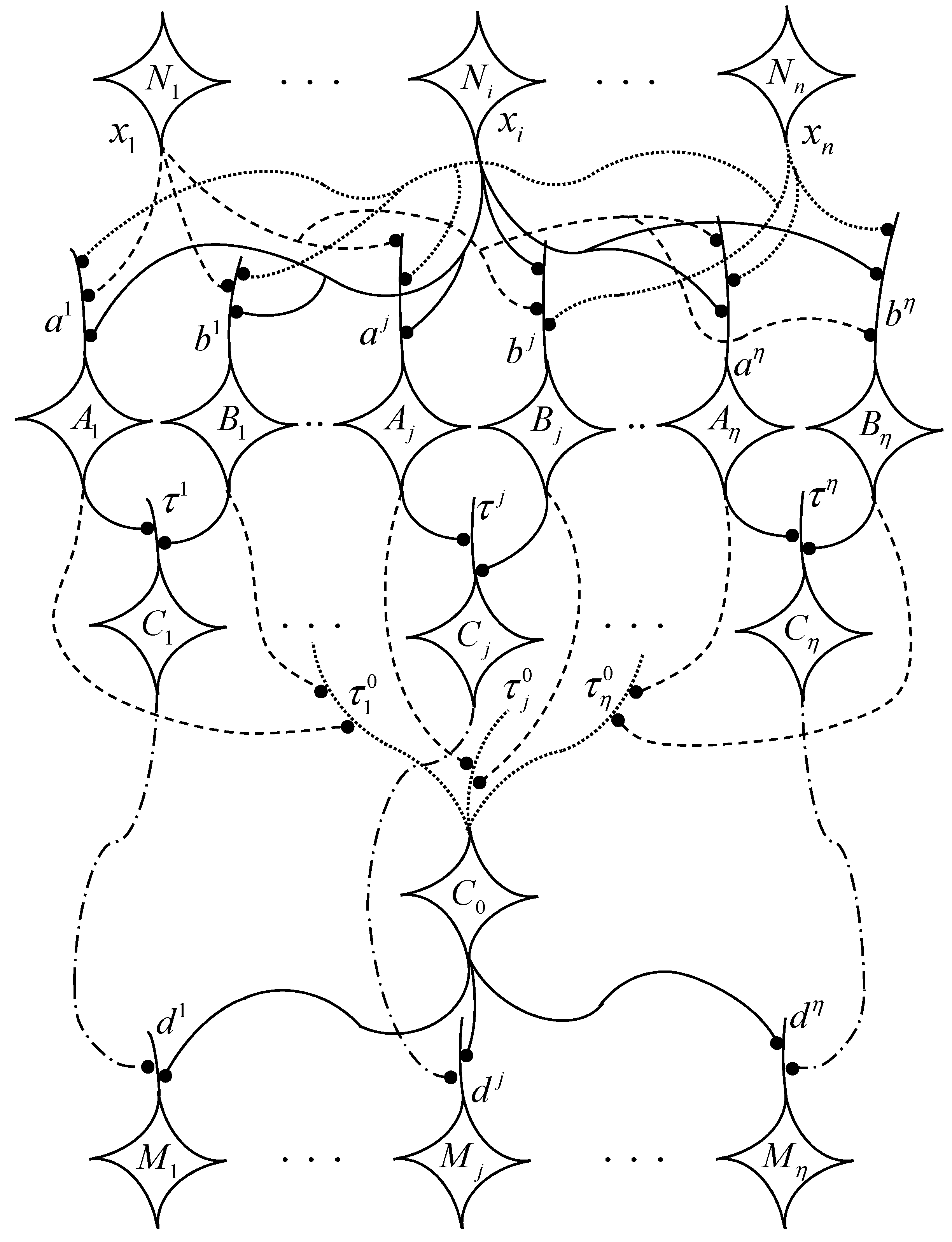
After selecting the training set $P_p$, precompute the values $v\left({\mathbf{q}}^{s_j}\right)={\sum }_{i=1}^n{q}_i^{s_j}$ for $j=1,\dots ,\eta$. These values will be stored at the synaptic sites of the LBNN and in most practical situations $\eta \gg n$. Knowing the dimension n and the size of the training set $P_p$, it is now an easy task to construct the network. As illustrated in Figure 2, the network has n input neurons denoted by $N_1,\dots ,N_n$, two hidden layer neurons, and a layer of output neurons. The first hidden layer neurons consist of two different types of neurons denoted by $A_j$ and $B_j$, where $j=1,\dots ,\eta$. Each neuron $A_j$ and $B_j$ will have a single dendrite with each dendrite having n synaptic sites. For the sake of simplicity we denote the dendrite of $A_j$ and of $B_j$ by $a^j$ and $b^j$, respectively. The second hidden layer has $\eta +1$ neurons denoted by $C_j$, where $j=0,1,\dots ,\eta$. Here $C_0$ has multiple dendrites, i.e., $\eta$ dendrites denoted by ${\tau }_j^0$, with each dendrite having two synaptic sites for $j=1,\dots ,\eta$. Any other neuron $C_j$ with $j\ne 0$ has one dendrite, with each dendrite having also two synaptic sites. The output layer is made up of $\eta$ neurons, denoted by $M_j$ for $j=1,\dots ,\eta$, with each neuron $M_j$ having a single dendrite with two synaptic sites.

In what follows, we describe the internal workings of the network. For a given $\mathbf{x}\in {\mathbb{R}}^{*}$, the input neuron $N_i$ receives the input $x_i$, and this information is sent to each of the neurons $A_j$ and $B_j$. For each $i=1,\dots ,n$, the axonal arborization of $N_i$ consists of $2\eta$ terminal branches with one terminal on each $a^j$ and $b^j$. The synaptic weight ${\alpha }_{ij}^{\ell }$ at the i-th synapse on $a^j$ is given by ${\alpha }_{ij}^{\ell }=q_i^{s_j}$ with $\ell =1$. Each synapse on $a^j$ at location $(i,j)$ results in $x_i\vee q_i^{s_j}$ upon receiving the information $x_i$. The total response of the dendrite $a^j$ is given by the summation $a^j\left(\mathbf{x}\right)=v(\mathbf{x}\vee {\mathbf{q}}^{s_j})={\sum }_{i=1}^n(x_i\vee q_i^{s_j})$. In a similar fashion, the synaptic weight ${\beta }_{ij}^{\ell }$ at the i-th synapse on $b^j$ is given by ${\beta }_{ij}^{\ell }=q_i^{s_j}$ with $\ell =1$. However, here, each synapse on $b^j$ at location $(i,j)$ results in $x_i\wedge q_i^{s_j}$ upon receiving the information $x_i$, and each neuron $B_j$ computes $b^j\left(\mathbf{x}\right)=v(\mathbf{x}\wedge {\mathbf{q}}^{s_j})={\sum }_{i=1}^n(x_i\wedge q_i^{s_j})$. This information $a^j\left(\mathbf{x}\right)$ and $b^j\left(\mathbf{x}\right)$ travels through the soma towards its axon hillock of the respective neurons where the corresponding activation functions are given, for $A_j$ and $B_j$ respectively, by:

$$f_j\left(\mathbf{x}\right)=\frac{v\left({\mathbf{q}}^{s_j}\right)}{v(\mathbf{x}\vee {\mathbf{q}}^{s_j})}\mathrm{and}{g}_j\left(\mathbf{x}\right)=\frac{v(\mathbf{x}\wedge {\mathbf{q}}^{s_j})}{v\left({\mathbf{q}}^{s_j}\right)}.$$

(17)

The information $f_j\left(\mathbf{x}\right)$ and $g_j\left(\mathbf{x}\right)$ is transferred via the axonal arborization of the first hidden layer neurons to the dendrites of the second layer neurons. The presynaptic neurons of $C_0$ are all the neurons of the first hidden layer. A terminal axonal fibers of $A_j$ and one from $B_j$ terminate on ${\tau }_j^0$. The weight at each of the two synapses is $w_{aj0}^{\ell }=0=w_{bj0}^{\ell }$, where $\ell =1$ and $aj$, $bj$ are address labels for the respective terminal axonal fibers from $A_j$ and $B_j$. Thus, each synapse accepts the information $f_j\left(\mathbf{x}\right)$ and $g_j\left(\mathbf{x}\right)$. The total response of the dendrite is given by ${\tau }_j^0\left(\mathbf{x}\right)=f_j\left(\mathbf{x}\right)\wedge g_j\left(\mathbf{x}\right)$. However, the total response of the neuron $C_0$ is given by:

$${\tau }^0\left(\mathbf{x}\right)=\underset{j=1}{\overset{\eta }{\bigvee }}{\tau }_j^0\left(\mathbf{x}\right)=\underset{j=1}{\overset{\eta }{\bigvee }}[f_j\left(\mathbf{x}\right)\wedge g_j\left(\mathbf{x}\right)]=\underset{j=1}{\overset{\eta }{\bigvee }}\left[\frac{v\left({\mathbf{q}}^{s_j}\right)}{v(\mathbf{x}\vee {\mathbf{q}}^{s_j})}\wedge \frac{v(\mathbf{x}\wedge {\mathbf{q}}^{s_j})}{v\left({\mathbf{q}}^{s_j}\right)}\right].$$

(18)

For $j=1,\dots ,\eta$, the presynaptic neurons for the neuron $C_j$ are the two neurons $A_j$ and $B_j$. Denoting the single dendrite of $C_j$ by ${\tau }^j$, then a terminal axonal fibers of $A_j$ and one from $B_j$ terminate on ${\tau }^j$. In lockstep with $C_0$, the weight at each of the two synapses is $w_{aj}^{\ell }=0=w_{bj}^{\ell }$, where $\ell =1$ and $aj$, $bj$ are address labels for the respective terminal axonal fibers from $A_j$ and $B_j$. Again, the two synapses accept the information $f_j\left(\mathbf{x}\right)$ and $g_j\left(\mathbf{x}\right)$, and the response of the single dendrite is:

$${\tau }^j\left(\mathbf{x}\right)=f_j\left(\mathbf{x}\right)\wedge g_j\left(\mathbf{x}\right)=\frac{v\left({\mathbf{q}}^{s_j}\right)}{v(\mathbf{x}\vee {\mathbf{q}}^{s_j})}\wedge \frac{v(\mathbf{x}\wedge {\mathbf{q}}^{s_j})}{v\left({\mathbf{q}}^{s_j}\right)}.$$

(19)

The activation function for $C_j$ is the identity function $f\left(\mathbf{x}\right)=\mathbf{x}$ for all $j\in \{0,1,\dots ,\eta \}$. For the output layer, the presynaptic neurons for $M_j$ are the two neurons $C_j$ and $C_0$. As mentioned earlier, each output neuron $M_j$ has one dendrite $d^j$ with two synaptic regions, one for the terminal axonal bouton of $C_j$ and one for $C_0$. The synaptic weight at the synapse of $C_j$ on $d^j$ is given by $w_j^{\ell }$, where $\ell =1$ and $w_j^1=0$, while the synaptic weight at the synapse of $C_0$ on $d^j$ is given by $w_0^{\ell }$, with $\ell =0$ and $w_0^0=0$.

Because the activation function of $C_j$ is the identity function, the input at the synapse with weight $w_j^1$ is ${\tau }^j\left(\mathbf{x}\right)$, and since $w_j^1=0$, the synapse accepts the input. Likewise, the input from neuron $C_0$ at the synapse with weight $w_0^0$ is ${\tau }^0\left(\mathbf{x}\right)$. However, because $\ell =0$, the weight negates the input since ${(-1)}^{(1-\ell )}[{\tau }^0\left(\mathbf{x}\right)+w_0^0]=-{\tau }^0\left(\mathbf{x}\right)$. The dendrite $d^j$ adds the results of the synapses so that, $d^j\left(\mathbf{x}\right)={\tau }^j\left(\mathbf{x}\right)-{\tau }^0\left(\mathbf{x}\right)$. This information flows to the hillock of $M_j$, and the activation function of $M_j$ is the hard-limiter $f\left[d^j\left(\mathbf{x}\right)\right]=1\iff d^j\left(\mathbf{x}\right)\ge 0$ and $f\left[d^j\left(\mathbf{x}\right)\right]=0$ if $d^j\left(\mathbf{x}\right)<0$.

Since ${\tau }^j\left(\mathbf{x}\right)\le {\tau }^0\left(\mathbf{x}\right)$ for $j=1,2,\dots ,\eta$, it follows that $f\left[d^j\left(\mathbf{x}\right)\right]=1\iff {\tau }^j\left(\mathbf{x}\right)={\tau }^0\left(\mathbf{x}\right)$. Suppose that ${\mathbf{q}}^{s_j}\in c_{\lambda }$ and $f\left[d^j\left(\mathbf{x}\right)\right]=1$. If for any $k\in \{1,\dots ,\eta \}\backslash \left\{j\right\}$, we have that $f\left[d^k\left(\mathbf{x}\right)\right]=0$, then we say that $\mathbf{x}\in c_{\lambda }$, i. e. winner takes all. If there is another winner that is not a member of $c_{\lambda }$, then repeat the steps with a new randomly obtained set $P_p$. If after several tries, a single winner cannot be found, it becomes necessary to increase the percentage of points in $P_p$. Note that the method just described can be simplified by eliminating the neuron $C_0$ and using the $C_1$ to $C_{\eta }$ neurons as the output neurons. If there is one ${\tau }^j\left(\mathbf{x}\right)$ such that ${\tau }^k\left(\mathbf{x}\right)<{\tau }^j\left(\mathbf{x}\right)$$\forall k\in \{1,\dots ,m\}\backslash \left\{j\right\}$, then $\mathbf{x}\in c_{\lambda }$, where $c_{\lambda }$ is the class of ${\mathbf{q}}^{s_j}$. If there is more than one winner where the other winner does belong to class $c_{\lambda }$, then repeat the steps with a new set $P_p$ as described earlier.

We close our theoretical description by pointing out the important fact that an extensive foundation with respect to the similarity measure given in Equation (16) or more precisely the two separate expressions in (17) has been developed earlier, although with a different perspective in mind, in related areas such as fuzzy sets [32,33,34], fuzzy logic [35,36], and fuzzy neural networks [37]. For example, the scalar lattice functions, defined by $f:L\to \mathbb{R}$ and $g:L\to \mathbb{R}$, where $f\left(x\right)=v\left(y\right)/v(x\vee y)$, $g\left(x\right)=v(x\wedge y)/v\left(y\right)$, and $v\left(x\right)=x$ for $y\in L$, were treated in [37]. Also, algorithms for computing subsethood and similarity for interval-valued fuzzy sets for the vectorial counterparts of f and g appear in [38].

5. Recognition Capability of Similarity Measure Based LNNs

Before discussing the issue of interest, we must mention that a previous LNN based on metrics appears in [39]. The proposed LBNN is trained in a fairly simple way in order to be able to recognize prototype-class associations in the presence of test or non-stored input patterns. As described in Section 4, the network architecture is designed to work with a finite set of hetero-associations, that we denote by $H\subset Q\times {\mathbb{N}}_m$. Using the prototype-class pairs of a training subset randomly generated from the complete data set, all network weights are preassigned. After weight assignment, non-stored input patterns chosen from a test set can be used to prove the memory network. A test set is defined as the complement of the training set of exemplar or prototype patterns. Clearly, test patterns are elements of one of the m classes that the LBNN can recognize. If the known class of a given non-stored pattern matches the net output class, correct classification or a hit occurs, otherwise an error of misclassification happens. Consequently, by computing the fraction of hits relative to each input set used to test the network we can measure the recognition capability of the proposed LBNN.

In the following paragraphs, some pattern recognition problems are examined to show the performance classification of our LBNN model based on the similarity measure given in (19). For each one of the examples described next, a group of prototype subsets $P_p$ were randomly generated by fixing increasing percentages $p\%$, of the total number k of samples in a given data set Q. Selected percentages p belong to the range $\{50\%,60\%,\dots ,90\%\}$ and generated test subsets, symbolized as $Q_p$, were obtained as complements of $P_p$ with respect to Q. Computation of the average fraction of hits for each selected percentage of all samples requires a finite number of trials or runs, here denoted by $\tau$. Let $\mu$ and ${\mu }_r$ be the average (over all runs) and the number of misclassified test patterns in each run, then the average fraction of hits is given by,

$$f_p^{\mathrm{hits}}=1-\frac{\mu }{k}\mathrm{where}\mu =\frac{1}{\tau }\sum _{r=1}^{\tau }{\mu }_r.$$

(20)

Note that, if $\left|Q\right|=k$, $|P_p|$, $|Q_p|$, are the cardinalities of the data, prototype, and test sets, respectively, then $k=|P_p|+|Q_p|$. In (20), we set the number of runs, $\tau =50$, for any percentage p of the training population sample in order to stabilize the mean value $\mu$. Although, for each run with the same value of p, the number of elements of $P_p$ and $Q_p$ does not change, the sample patterns belonging to each subset are different since they are selected in random fashion. Also, observe that a lattice biomimetic net trained for some p with a prototype subset $P_p$, can be tested either with the whole data set $Q=P_p\cup Q_p$ or with the test set $Q_p$.

We will use a table format to display the computational results obtained for LBNN learning and classification of patterns for the example data sets, to give the mean capability performance in recognizing any element in Q. Each table is composed of six columns; the first column gives the dataset characteristics; the second column gives the percentage p of sample patterns used to generate the prototype and test subsets; the third column provides the number of randomly selected prototype patterns, and the fourth column gives the number of test patterns. The fifth column shows the average number of misclassified inputs calculated using the similarity lattice valuation measure and the sixth column gives the corresponding average fraction of hits for correct classifications.

5.1. Classification Performance on Artificial Datasets

The following two examples are designed to illustrate simple data sets with two and three attributes that can be represented graphically as scatter plots, respectively, in two and three dimensions. We remark that both sets are build artificially and do not correspond to data sets coming from realistic measurements taken from a real-world situation or application.

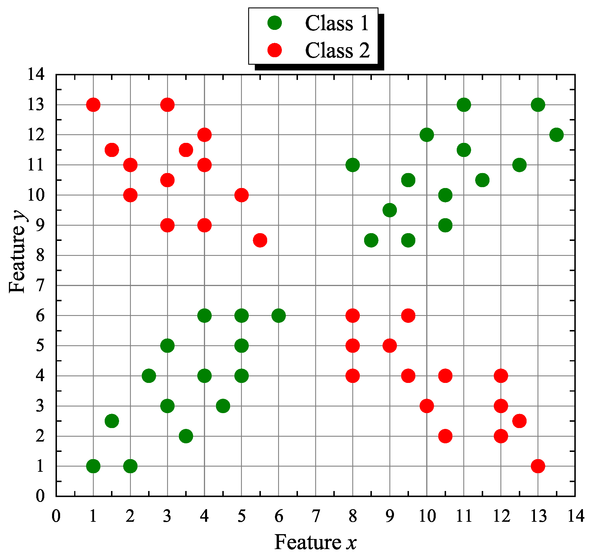
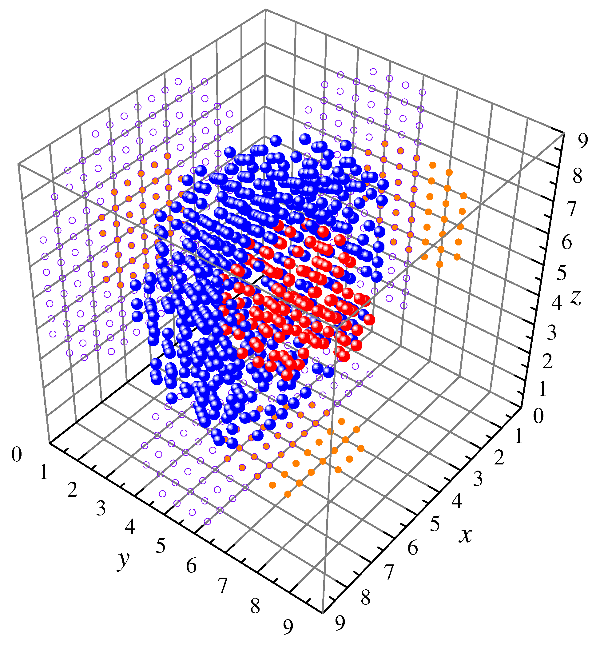
Our first artificial or synthetic data set Q forms a discrete planar “X” shape with 55 points (samples) where coordinates x and y correspond to its two features. The points are distributed in two classes $c_{\lambda }$ where $\lambda \in \{1,2\}$. The corresponding 2D scatter plot is shown in Figure 3. Similarly, the second synthetic set Q consists of 618 samples defined in the first octant of ${\mathbb{R}}^3$. Points in class $c_1$ belong randomly to a hemisphere of radius $3.5$ centered at $(5,5,5)$ with a hemispherical cavity of radius $1.5$ concentric to the larger hemisphere and class $c_2$ points belong, also randomly, to a sphere of radius $1.5$ embedded in the cavity formed by class $c_1$ points. Again, features are specified by the x, y, and z coordinates and the corresponding three-dimensional scatter plot is depicted in Figure 4.

Table 1. Similarity valuation LBNN classification performance for the “X-shaped” (X-s) and “hemisphere-sphere” (H-s) datasets.

Q	p	$|{\mathit{P}}_{\mathit{p}}|$	$|{\mathit{Q}}_{\mathit{p}}|$	$\lfloor {\mathit{\mu }}_{\mathit{p}}\rfloor$	${\mathit{f}}_{\mathit{p}}^{\mathbf{hits}}$
X-s	$50\%$	28	27	0	0.994
$k=55$	$60\%$	33	22	0	0.998
$m=2$	$70\%$	39	16	0	0.999
$n=2$	$80\%$	44	11	0	1.000
	$90\%$	50	5	0	1.000
H-s	$50\%$	309	309	13	0.978
$k=618$	$60\%$	370	248	11	0.982
$m=2$	$70\%$	432	186	8	0.987
$n=3$	$80\%$	494	124	5	0.992
	$90\%$	556	62	2	0.996

gives the numerical results for the “X-shape” (X-s) and “Hemisphere-sphere” (H-s) datasets.

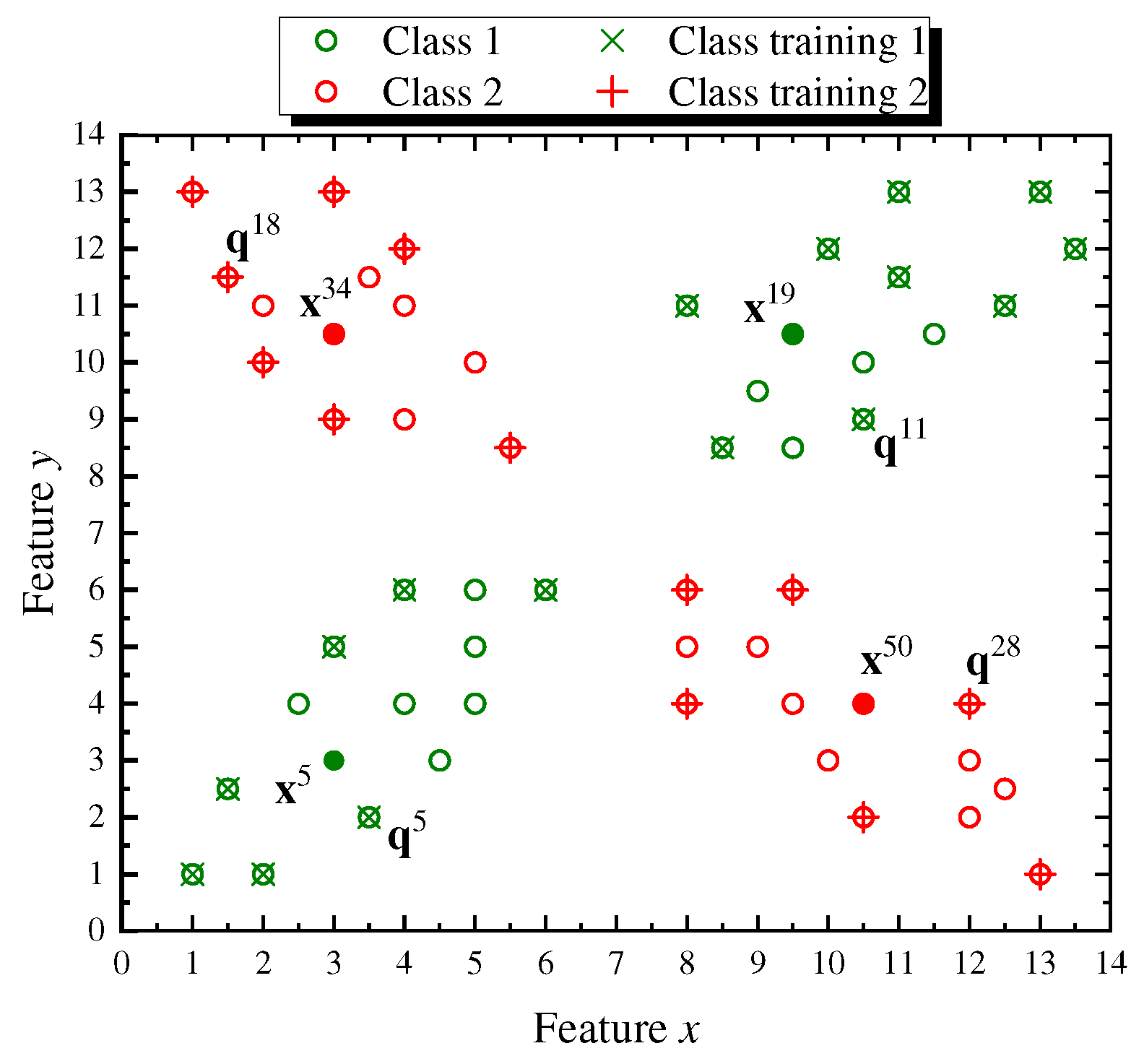
The last column in Table 1 shows the high classification rates achieved by training the similarity valuation based LBNN with, at least half the number of samples, and repeating the learning procedure several times in random fashion. For the sake of completeness, we explain graphically, using the X-shaped dataset, how the lattice based neural network shown in Figure 2 assigns a class label to input patterns once the network is trained with a randomly generated prototype subset $P_p$ of Q setting $p=55\%$. Specifically, Figure 5 displays the $k=55$ points in Q that form the X-shaped set, where the point circles crossed with the symbol “×” (in olive green) denote class $c_1$ training data and the point circles marked with a “+” sign (over the red circles) are class $c_2$ training data totaling 29 elements belonging to $P_p$. In the same figure, test points ${\mathbf{x}}^5$, ${\mathbf{x}}^{19}$, ${\mathbf{x}}^{34}$, and ${\mathbf{x}}^{50}$, selected from the 26 elements of $Q_p$, are shown as filled colored dots and its class is determined based on the neural similarity lattice valuation measure response given in (18).

As can be seen in Figure 5, class $\lambda =1$ is correctly attached to the test points, ${\mathbf{x}}^5=(3,3)$ and ${\mathbf{x}}^{19}=(9.5,10.5)$, since the maximum similarity valuation measure computed using (18), is obtained, respectively, for the training points, ${\mathbf{q}}^5=(3.5,2)$ and ${\mathbf{q}}^{11}=(10.5,9)$, which are elements of $c_1$. Analogously, class $\lambda =2$ is correctly assigned to the test points, ${\mathbf{x}}^{34}=(3,10.5)$ and ${\mathbf{x}}^{50}=(10.5,4)$, since the maximum similarity valuation measure is found for the training points, ${\mathbf{q}}^{18}=(1.5,11.5)$ and ${\mathbf{q}}^{28}=(12,4)$, data elements of $c_2$. More specifically, the explicit calculation expression corresponding to (18) for testing any point ${\mathbf{x}}^{\zeta }\in Q_p$ is given by,

$${\tau }^0\left({\mathbf{x}}^{\zeta }\right)=\underset{j=1}{\overset{29}{\bigvee }}\left[\frac{q_1^j+q_2^j}{(x_1^{\zeta }\vee q_1^j)+(x_2^{\zeta }\vee q_2^j)}\wedge \frac{(x_1^{\zeta }\wedge q_1^j)+(x_2^{\zeta }\wedge q_2^j)}{q_1^j+q_2^j}\right].$$

(21)

We end our discussion about the X-shaped artificial dataset by showing the similarity valuation measure graphs of the selected test points, ${\mathbf{x}}^5,{\mathbf{x}}^{19},{\mathbf{x}}^{34},{\mathbf{x}}^{50}\in Q_p$. Hence, Figure 6 displays from top to bottom the similarity measure curves whose domain is the data training subset $P_p$ and with values ranging on the interval $[0,1]$. The maximum similarity value ${\tau }^0\left({\mathbf{x}}^{\zeta }\right)$ is represented with the symbol ▿ and the corresponding training pattern index within the set $P_p$ is found at the bottom of the dropped vertical line (dashed). The LBNN then assigns the correct class to each one of the selected test points as depicted in the same figure with respect to the line dividing both classes.

5.2. Classification Performance on Real-World Application Datasets

Various application examples available at the UCI Machine Learning Repository [40] are described and discussed in this subsection in order to exhibit the similarity valuation LBNN classification performance. The numeric results are compiled in

Table 2. Similarity valuation LBNN classification performance for the application datasets.

Q	p	$|{\mathit{P}}_{\mathit{p}}|$	$|{\mathit{Q}}_{\mathit{p}}|$	$\lfloor {\mathit{\mu }}_{\mathit{p}}\rfloor$	${\mathit{f}}_{\mathit{p}}^{\mathbf{hits}}$
Iris	$50\%$	75	75	3	0.975
$k=150$	$60\%$	90	60	2	0.980
$m=3$	$70\%$	105	45	2	0.987
$n=4$	$80\%$	120	30	1	0.991
	$90\%$	135	15	0	0.997
Column	$50\%$	155	155	33	0.893
$k=310$	$60\%$	186	124	25	0.917
$m=3$	$70\%$	217	93	19	0.939
$n=6$	$80\%$	248	62	13	0.958
	$90\%$	279	31	6	0.981
Wine	$50\%$	89	89	23	0.871
$k=178$	$60\%$	107	71	17	0.902
$m=3$	$70\%$	125	53	12	0.930
$n=13$	$80\%$	142	36	8	0.956
	$90\%$	160	18	4	0.978

that has the same organization as explained in the previous subsection on artificial datasets. However, in Table 2 each block of rows in a given example is separated by a horizontal line.

Example 1.

The “Iris” dataset has 150 samples where each sample is described by four flower features (sepal length, sepal width, petal length, petal width) and is equally distributed into three classes $c_1$, $c_2$, and $c_3$, corresponding, respectively, to the subspecies of Iris setosa, Iris versicolor, and Iris virginica. A high average fraction of hits such as $f_p^{hits}>0.97$ is obtained for percentages $p\ge 50\%$. The similarity valuation trained LBNN used as an individual classifier delivers similar performance against linear or quadratic Bayesian classifiers [41] for which $f_{50}^{hits}=0.953$ and $f_{50}^{hits}=0.973$, respectively, or in comparison with an edge-effect fuzzy support vector machine [42] whose $f_{60}^{hits}=0.978$.

Example 2.

The “Column” dataset with 310 patient samples is specified by six biomechanical attributes derived from the shape and orientation of the pelvis and lumbar spine. Attributes 1 to 6 are numerical values of pelvic incidence, pelvic tilt, lumbar lordosis angle, sacral slope, pelvic radius, and grade of spondylolisthesis. Class $c_1$ of patients diagnosed with disk hernia has 60 samples, class $c_2$ of patients diagnosed with spondylolisthesis 150 samples, and class $c_3$ of normal patients 100 samples. Since feature 6 has several negative entries, the whole set is displaced to the positive octant of ${\mathbb{R}}^3$ by adding $|inf(Q\left)\right|=11.06$ to every vector in Q. In this case, a high average fraction of hits occurs for percentages p greater than $80\%$, which is due to the presence of several interclass outliers. However, the LBNN with much less computational effort is still good if compared with other classifiers such as an SVM (support vector machine) or a GRNN (general regression neural network) [43] (with all outliers removed), which both give $f_{80}^{hits}=0.965$.

Example 3.

The “Wine” dataset has 178 samples subject to chemical analysis of wines produced from three different cultivars (classes) of the same region in Italy. The features in each sample represent the quantities of 13 constituents: alcohol, malic acid, ash, alkalinity of ash, magnesium, phenols, flavonoids, nonflavonoid phenols, proanthocyanins, color intensity, hue, diluted wines, and proline. Class $c_1$ has 59 samples, class $c_2$ 71 samples, and class $c_3$ 48 samples. In this last example, a high average fraction of hits occurs for percentages p greater than $80\%$, and the LBNN performance is quite good if compared with other classifiers, based on the leave one-out technique, such as the 1-NN (one-nearest neighbor), LDA (linear discriminant analysis), and QDA (quadratic discriminant analysis) [44], which give, correspondingly, $f_p^{hits}=0.961$, $f_p^{hits}=0.989$, and $f_p^{hits}=0.994$, where $p=99.44\%$, and training must be repeated $\tau =178$ times. Although not shown in Table 2, the LBNN net gives $f_{99}^{hits}\simeq 1$, since almost all samples in the given dataset are stored by the memory as prototype patterns. However, our LBNN model is outperformed by a short margin of misclassification error ($0.055$), since $f_{75}^{hits}=0.942$, if compared to an FLNN classifier (fuzzy lattice neural network) that gives $f_{75}^{hits}=0.997$ (leave-25%-out) [45].

6. Conclusions

This paper introduces a new lattice based biomimetic neural network structured as a two hidden layer dendritic lattice hetero-associative memory whose total neural response is computed using a similarity measure derived from a lattice positive valuation. The proposed model delivers a high ratio of successful classification for any data pattern considering that the network learns random prototype patterns with a percentage level from $50\%$ up to $90\%$ of the total number of patterns belonging to a data set.

More specifically, the new LBNN model provides intrinsic capacity to tackle multivariate- multiclass problems in pattern recognition pertaining to applications whose features are specified by data measured numerically. Our network model incorporates a straightforward mechanism whose topology implements a similarity function defined by simple lattice arithmetical operation used to measure the resemblance between a set of n-dimensional real vectors (prototype patterns) and a test input n-dimensional vector, in order to match its class. Representative examples, such as the “Iris”, the “Column”, and the “Wine” datasets, were used to carry on several computational experiments to obtain the average classification performance of the proposed LBNN for diverse randomly generated test subsets. Furthermore, the proposed LBNN model can be applied in other areas such as cryptography [46] or image processing [47,48,49,50].

The results given in this paper are competitive and look promising. However, future work with the LBNN classifier contemplates computational enhancements and comparisons with other challenging artificial and experimental data sets. Additionally, further analysis is required to deal with important issues such as data test set design, theoretical developments based on different lattice valuations, and comparisons with recently developed models based on lattice computing. We must point out that our classification performance experiments are actually limited due to its implementation in standard high-speed sequential machines. Nonetheless, LBNNs as described here and in early writings, can work in parallel using dedicated software or implemented in hardware to increase computational performance. Hence, a possible extension is to consider algorithm parallelization using GPUs or hardware realization as a neuromorphic system.