Dynamics of a SIR Epidemic Model of Childhood Diseases with a Saturated Incidence Rate: Continuous Model and Its Nonstandard Finite Difference Discretization

Abstract

A SIR epidemic model that describes the dynamics of childhood disease with a saturated incidence rate and vaccination program at a constant rate was investigated. For the continuous model we first show its basic properties, namely, the non-negativity and boundedness of solutions. Then we investigate the existence and both local and global stability of the equilibrium points. It was found that the existence and stability properties of equilibrium points fully determined the basic reproduction number. We also propose and analyze a discrete-time analogue of the continuous childhood diseases by applying a nonstandard finite difference method. It is shown that our discrete model preserves the dynamical properties of the corresponding continuous model, such as the positivity solutions, the population conservation law, the existence of equilibrium points and their global stability properties.

1. Introduction

One of the major issues in public health problems is childhood diseases (measles, mumps, influenza, smallpox, chickenpox, Rubella, Polio, etc.), which can spread rapidly among children age 5 and below due to frequent contact with their peers at school or elsewhere. For childhood diseases, vaccination is considered as an effective control strategy against childhood diseases. To understand the transmission dynamics of childhood diseases, Makinde [1] considered a SIR epidemic model which includes three sub-populations, namely, the susceptible sub-population $\left(S\right)$, the infective sub-population $\left(I\right)$ and the recovered sub-population $\left(R\right)$. The influence of a preventive vaccine is modeled by assuming that there exists a fraction of the susceptible population vaccinated at birth each year. The incidence rate of infection in this model is assumed to be bi-linear, i.e., $bSI$, where b is a parameter that measures the disease transmission rate. However, when an epidemic occurs in a large population, there are changes in people’s behavior to prevent infection (known as the crowding effect [2,3,4,5]) and hence the bi-linear incidence rate cannot be applied anymore. To consider such behavioral changes, Anderson and May [6] proposed a saturated incidence rate $\frac{1}{1+aI}$, where a is the inhibitory constant. The infection rate clearly decreases as the constant of inhibition increases, and in response to increasing the preventive measures and proper awareness.

In this paper, we modify the model in [1] by considering a saturated incidence rate. The compartment diagram of the proposed model is illustrated in Figure 1. One of the important preventive measures in the spread of childhood disease is vaccination. Therefore, we introduce an additional parameter $\theta$ to represent the fraction of individuals vaccinated at birth each year where $0\le \theta \le 1$. The SIR epidemic model of childhood diseases with saturated incidence rate and constant vaccination strategy is

$$\begin{array}{ccc}\frac{dS}{dt}& =& (1-\theta )A-\frac{bSI}{1+aI}-mS\hfill \\ \frac{dI}{dt}& =& \frac{bSI}{1+aI}-(m+g+e)I\hfill \\ \frac{dR}{dt}& =& \theta A+gI-mR,\hfill \end{array}$$

(1)

where A is the constant recruitment rate; m and e are the natural death rate and the death rate caused by the disease, respectively; and g represents the recovery rate. It is assumed that the initial values of system (1) are non-negative, namely, $S\left(0\right)=S_0\ge 0,I\left(0\right)=I_0\ge 0$ and $R\left(0\right)=R_0\ge 0$.

From a mathematical point of view, Makinde [1] has provided a qualitative analysis for the SIR model with a bi-linear incidence rate. He also applied the Adomian decomposition method to obtain an analytical approximation to its solutions. Another analytical approximation to this problem has also been introduced by Yildirim and Cherruault [7], namely, by using the homotopy perturbation method. On the other hand, it is often desirable to get quantitative solutions and therefore the epidemic model has to be discretized. In this case, the obtained numerical scheme has to maintain the dynamical properties of the corresponding continuous model. For this purpose, Mickens [8] has introduced a nonstandard finite difference (NSFD) method, which has two characteristics:

(i)

The first order derivative in the continuous model is approximated by the generalized forward difference

$$\frac{d{x}_n}{dt}\approx \frac{x_{n+1}-x_n}{\phi \left(h\right)},$$

where $x_n=x\left(t_n\right)$ and $\phi \left(h\right)$ is the denominator function such that $\phi \left(h\right)=h+\mathcal{O}\left(h^2\right)$ with h as the time-step size.

(ii)

The nonlinear terms are approximated non-locally.

The NSFD method has been applied successfully in various problems, including in ecology [9,10,11,12] and epidemiology [13,14,15,16,17,18,19]. Recently, Cui et al. [20] constructed a NSFD scheme for the SIR epidemic model of childhood diseases with bi-linear incidence rate and showed that the resulting discrete system is dynamically consistent with the original continuous model.

For all we know, the dynamics of the SIR epidemic model (1) and its discrete version have not been studied. Hence, the SIR epidemic model of childhood diseases with saturated incidence rate and constant vaccination strategy is proposed and the dynamics are investigated in this paper. We first discuss the basic properties of the model such as the non-negativity solutions and the population conservation law. We also provide local and global stability analysis for all possible equilibrium points. Then, we construct an NSFD scheme for the model (1) and investigate the dynamics of the obtained discrete model. The dynamics of the discrete model are compared to the continuous model to check their consistency.

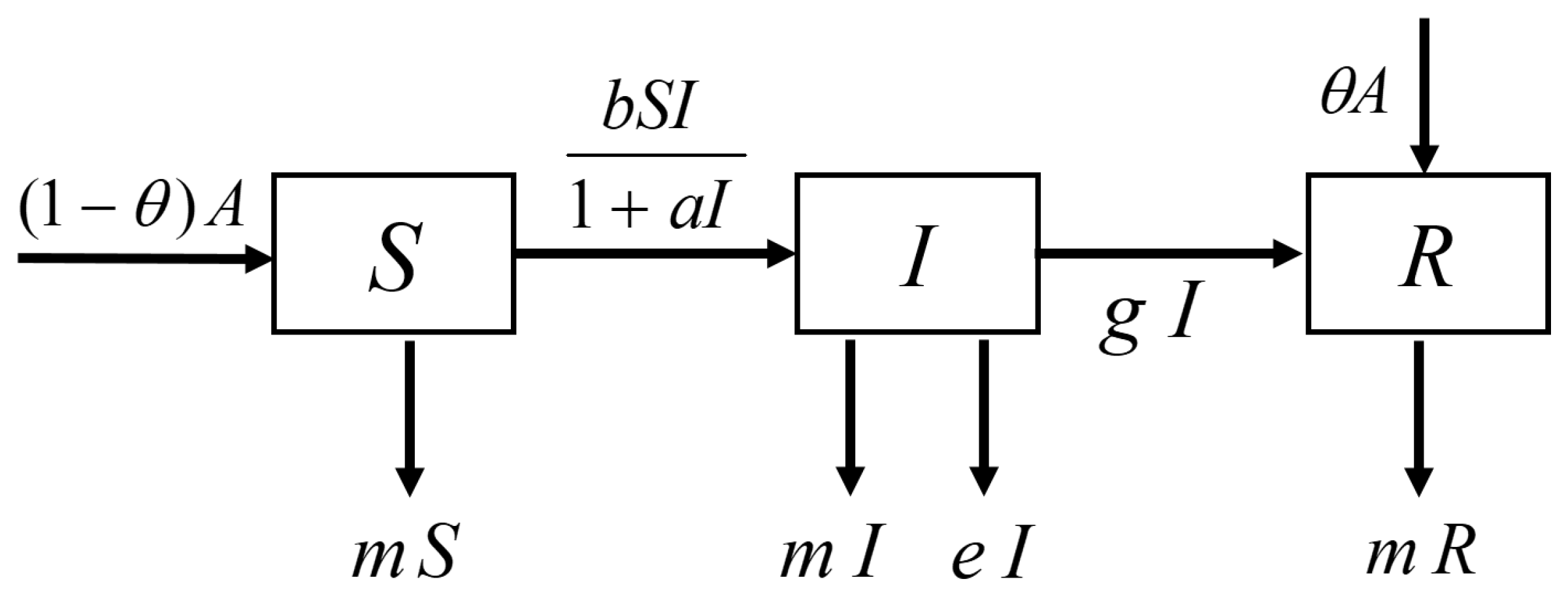
2. Dynamics of the Continuous Epidemic Model of Childhood Diseases

2.1. Basic Properties of the Continuous Model

Since we are considering a model of population dynamics, all solutions of model (1) must be non-negative. Furthermore, due to the limited resources, the size of the population has to be bounded. In the following theorem, we prove the non-negativity and the boundedness of solutions of system (1).

Theorem 1.

All solutions of system (1) with non-negative initial values are always non-negative and uniformly bounded.

Proof. 

From system (1) and the non-negativity of initial values $S_0\ge 0,I_0\ge 0$ and $R_0\ge 0$, we have

$$\begin{array}{ccc}{\displaystyle S\left(t\right)}& =& S\left(0\right)exp{\int }_0^t\left((1-\theta )A-\frac{bS\left(z\right)I\left(z\right)}{1+aI\left(z\right)}-mS\left(z\right)\right)dz\ge 0\hfill \\ {\displaystyle I\left(t\right)}& =& I\left(0\right)exp{\int }_0^t\left(\frac{bS\left(z\right)I\left(z\right)}{1+aI\left(z\right)}-(m+g+e)I\left(z\right)\right)dz\ge 0\hfill \\ {\displaystyle R\left(t\right)}& =& R\left(0\right)exp{\int }_0^t\left(\theta A+gI\left(z\right)-mR\left(z\right)\right)dz\ge 0.\hfill \end{array}$$

(2)

Hence all solutions of system (1) are always non-negative. Next, if we define the total population as $T\left(t\right)=S\left(t\right)+I\left(t\right)+R\left(t\right)$, then system (1) gives the following population conservation law (see [14,21] for the detail terminology of population conservation law):

$$\frac{dT}{dt}=A-mT-eI\le A-mT.$$

(3)

Using the Gronwall’s inequality, we get

$$T\left(t\right)\le \frac{A}{m}+\left(T_0-\frac{A}{m}\right)exp(-mt),$$

(4)

where $T_0=S_0+I_0+R_0$. Hence ${lim}_{t\to +\infty }T\left(t\right)\le \frac{A}{m}$, which shows that the solutions of system (1) are uniformly bounded. □

It is easy to show that system (1) always has a disease free equilibrium (DFE) point $E^0=\left(S^0,0,R^0\right)$, where $S^0=(1-\theta )A/m$ and $R^0=\theta A/m$. Furthermore, if ${\mathcal{R}}_0>1$, then the system also has a unique endemic equilibrium (EE) point $E^{*}=\left(S^{*},I^{*},R^{*}\right)$ where $S^{*}=\frac{(b+am{\mathcal{R}}_0)(1-\theta )A}{m{\mathcal{R}}_0(am+b)},I^{*}=\frac{m({\mathcal{R}}_0-1)}{am+b}$ and $R^{*}=(\theta A+g{I}^{*})/m$. Here

$${\mathcal{R}}_0=\frac{(1-\theta )Ab}{m(m+g+e)}$$

(5)

denotes the basic reproduction number which can be determined easily using the next generation matrix method; see [22]. In the following part, we investigate the local and global stability of the existing equilibrium points. Since the first two equations of system (1) do not depend on R, it is enough to consider the following reduced system

$$\begin{array}{ccc}{\displaystyle \frac{dS}{dt}}& =& {\displaystyle (1-\theta )A-\frac{bSI}{1+aI}-mS=f_1(S,I)}\hfill \\ {\displaystyle \frac{dI}{dt}}& =& {\displaystyle \frac{bSI}{1+aI}-(m+g+e)I=f_2(S,I).}\hfill \end{array}$$

(6)

2.2. Local Stability Analysis of the Continuous Model

To study the local stability of each equilibrium point, we examine the eigenvalues of the Jacobian matrix of the system (6) at each equilibrium point. The Jacobian matrix of system (6) at $E^0=(S^0,0)$ is

$$J\left(E^0\right)=\left[\begin{array}{cc}-m& -b{S}^0\\ 0& b{S}^0-(m+g+e)\end{array}\right].$$

(7)

The eigenvalues of $J\left(E^0\right)$ are ${\lambda }_1=-m<0$ and ${\lambda }_2=b{S}^0-(m+g+e)$. We observe that ${\lambda }_2<0$ if ${\mathcal{R}}_0<1$ and ${\lambda }_2>0$ whenever ${\mathcal{R}}_0>1$. Hence, the DFE is locally asymptotically stable (L.A.S.) if ${\mathcal{R}}_0<1$ and it is unstable if ${\mathcal{R}}_0>1$. Next, we note that the Jacobian matrix at the EE point $E^{*}=(S^{*},I^{*})$ is given by

$$J\left(E^{*}\right)=\left[\begin{array}{cc}-m-\frac{b{I}^{*}}{1+a{I}^{*}}& -\frac{m+g+e}{1+a{I}^{*}}\\ \frac{b{I}^{*}}{1+a{I}^{*}}& \frac{m+g+e}{1+a{I}^{*}}-(m+g+e)\end{array}\right],$$

(8)

from which we get

$$det\left(J\left(E^{*}\right)\right)=\frac{(b+am)I^{*}}{1+a{I}^{*}}>0,$$

and

$$\mathrm{trace}\left(J\left(E^{*}\right)\right)=-\frac{a(m+g+e){\left(I^{*}\right)}^2+m{\mathcal{R}}_0}{I^{*}(1+a{I}^{*})}<0.$$

Thus, the real parts of all eigenvalues of the system(6) are negative, and consequently, the EE point is L.A.S. The local stability of equilibrium points of system (6) is summarized in the following theorem.

Theorem 2.

1. 

The DFE point $\left(E^0\right)$ is L.A.S.if ${\mathcal{R}}_0<1$ and is unstable if ${\mathcal{R}}_0>1$.

2. 

The EE point $\left(E^{*}\right)$ is L.A.S. if ${\mathcal{R}}_0>1$.

2.3. Global Stability Analysis of the Continuous Model

In this section, we discuss the global stability of equilibrium points. The global stability of the DFE point is shown by choosing a suitable Lyapunov function and employing the La Salle invariance principle, while that of the EE point is proven by defining a Dulac function and applying the Poincaré–Bendixson theory. The sufficient conditions for the global stability of both equilibrium points are stated in the following theorems.

Theorem 3.

The DFE point $\left(E^0\right)$ is globally asymptotically stable (GAS) if ${\mathcal{R}}_0\le 1$.

Proof. 

We first consider a Lyapunov function ${\mathcal{L}}_1=S-S^0-S^{0}ln\left(\frac{S}{S^0}\right)+I$. Using system (1), the time derivative of our Lyapunov function is given by

$$\begin{array}{ccc}\frac{d{\mathcal{L}}_1}{dt}& =& \left(1-\frac{S^0}{S}\right)\frac{dS}{dt}+\frac{dI}{dt}\hfill \\ & =& \frac{1}{S}(S-S^0)\left((1-\theta )A-\frac{bSI}{1+aI}-mS\right)+\left(\frac{bSI}{1+aI}-(m+g+e)I\right)\hfill \\ & =& -\frac{m}{S}{(S-S^0)}^2+\left(\frac{b{S}^{0}I}{1+aI}-(m+g+e)I\right)\hfill \\ & =& -\frac{m}{S}{(S-S^0)}^2-(m+g+e)\left(1-\frac{{\mathcal{R}}_0}{1+aI}\right)I\hfill \end{array}$$

Notice that we have applied relation $(1-\theta )A=m{S}^0$. It is obvious that $\frac{d{\mathcal{L}}_1}{dt}<0$ if ${\mathcal{R}}_0\le 1$ for all $(S,I)\ne (S^0,0)$. In addition, $\frac{d{\mathcal{L}}_1}{dt}=0$ if and only if $(S,I)=(S^0,0)$, showing that singleton $\left\{E^0\right\}$ is the only invariant set for which $\frac{d{\mathcal{L}}_1}{dt}=0$. Hence, the La Salle invariance principle states that the DFE point of system (1) is GAS. □

Theorem 4.

If ${\mathcal{R}}_0>1$, then the EE point $\left(E^{*}\right)$ is GAS.

Proof. 

It has been shown previously that $E^{*}$ is L.A.S. if ${\mathcal{R}}_0>1$. Next, we show the system (6) has no closed-orbit. For that, we define a Dulac function as follows:

$$\mathcal{B}(S,I)=\frac{1+aI}{I}.$$

Then, we have that

$$\begin{array}{ccc}\frac{\partial \left(\mathcal{B}{f}_1\right)}{\partial S}+\frac{\partial \left(\mathcal{B}{f}_2\right)}{\partial I}& =& \frac{\partial }{\partial S}\left(\frac{(1-\theta )(1+aI)A}{I}-bS-\frac{m(1+aI)S}{I}\right)+\frac{\partial }{\partial I}\left(bS-(m+g+e)(1+aI)\right)\hfill \\ & =& -\left(b+a(2m+g+e)+\frac{m}{I}\right)<0.\hfill \end{array}$$

Thus, system (6) or equivalently system (1) does not have a closed orbit. Since the EE point $\left(E^{*}\right)$ is L.A.S. if ${\mathcal{R}}_0>1$, then using the Poincaré–Bendixson theory we conclude that $\left(E^{*}\right)$ is GAS if ${\mathcal{R}}_0>1$. □

3. Dynamics of the Discrete NSFD Epidemic Model of Childhood Diseases

3.1. Construction of the Discrete NSFD Model

To get a dynamically-consistent numerical scheme, in this section we apply the NSFD method to discretize system (1). Here, the numerical approximations of $S\left(t\right),I\left(t\right)$ and $R\left(t\right)$ at $t=nh,n=0,1,2,\dots$ are respectively denoted by $S_n,I_n$ and $R_n$, where h is the time-step size. Following Mickens [8], we employ a generalized forward difference and nonlocal approximation for system (1):

$$\begin{array}{ccc}{\displaystyle \frac{S_{n+1}-S_n}{\phi \left(h\right)}}& =& {\displaystyle (1-\theta )A-\frac{b{S}_{n+1}{I}_n}{1+a{I}_n}-m{S}_{n+1}}\hfill \\ {\displaystyle \frac{I_{n+1}-I_n}{\phi \left(h\right)}}& =& {\displaystyle \frac{b{S}_{n+1}{I}_n}{1+a{I}_n}-(m+g+e)I_{n+1}}\hfill \\ {\displaystyle \frac{R_{n+1}-R_n}{\phi \left(h\right)}}& =& {\displaystyle \theta A+g{I}_{n+1}-m{R}_{n+1},}\hfill \end{array}$$

(9)

where $\phi \left(h\right)$ is the denominator function. As in the previous continuous model, we also consider a non-negative initial values $S_0\ge 0,I_0\ge 0$ and $R_0\ge 0$. By adding all equations in the scheme (9), we get

$${\displaystyle \frac{T_{n+1}-T_n}{\phi \left(h\right)}=A-m{T}_{n+1}-e{I}_{n+1}\le A-m{T}_{n+1},}$$

(10)

where $T_n=S_n+I_n+R_n$. It can be seen that Equation (10) is the approximation for the continuous population conservation law (3). To satisfy the exact population conservation law, we choose the following denominator function:

$$\phi \left(h\right)=\frac{exp\left(mh\right)-1}{m}.$$

(11)

Notice that we have implemented a nonlocal approximation for the right hand sides of system (1) and the denominator function satisfies $\phi \left(h\right)=h+\mathcal{O}\left(h^2\right)>0$ for all $h>0$. Hence, scheme (10) and scheme (9) are considered to be the NSFD scheme. Furthermore, if the denominator function (11) is substituted into the inequality (10) then we can easily show that

$${\displaystyle T_{n+1}\le \frac{A}{m}+\left(T_n-\frac{A}{m}\right)exp(-mh).}$$

(12)

Based on inequality (12), we can prove using mathematical induction that for any $h>0$ the solution of Equation (10) with the denominator function (11) satisfies the exact population conservation law (4):

$$T_n\le \frac{A}{m}+\left(T_0-\frac{A}{m}\right)exp(-mnh).$$

(13)

The NSFD scheme (9) is implicit, but it can be written in an explicit form as follows:

$$\begin{array}{ccc}{\displaystyle S_{n+1}}& =& {\displaystyle \frac{S_n+\phi \left(h\right)(1-\theta )A}{1+\phi \left(h\right)\left(m+{\Phi }_n\right)}}\hfill \\ {\displaystyle I_{n+1}}& =& {\displaystyle \frac{I_n+\phi \left(h\right){\Phi }_n{S}_{n+1}}{1+\phi \left(h\right)\left(m+g+e\right)}}\hfill \\ {\displaystyle R_{n+1}}& =& {\displaystyle \frac{R_n+\phi \left(h\right)\left(\theta A+g{I}_{n+1}\right)}{1+\phi \left(h\right)m},}\hfill \end{array}$$

(14)

where $\Phi \left(x\right)=\frac{bx}{1+ax}$ and ${\Phi }_n=\Phi \left(I_n\right)$. By remembering that the initial values are non-negative, $\phi \left(h\right)>0$ and all parameters are positive with $0\le \theta \le 1$, it is easily seen that ${\Phi }_0\ge 0$ and $S_1\ge 0$. Consequently, we also have $I_1\ge 0$ and $R_1\ge 0$. By applying this procedure consecutively for all n, we conclude that numerical solutions of system (14) are always non-negative: $S_n\ge 0,I_n\ge 0$ and $R_n\ge 0$ for all $n>0$ and for any $h>0$.

Using standard calculations, we can verify that the discrete NSFD model (14) always has a DFE point $E^0=(S^0,0,R^0)$. If ${\mathcal{R}}_0>1$, then the discrete system (14) also has a unique EE point $E^{*}=\left(S^{*},I^{*},R^{*}\right)$. These equilibrium points and their existence conditions are exactly the same as those of the continuous model (1), irrespective of h. In the following sub-sections we investigate the stability of those equilibrium points.

3.2. Local Stability Analysis of the Discrete NSFD Model

We notice that the first two equations in system (14) are independent of variabel $R_n$. Hence, for the stability analysis, we can consider the following reduced discrete NSFD model

$$\begin{array}{ccc}{\displaystyle S_{n+1}}& =& {\displaystyle \frac{S_n+\phi \left(h\right)(1-\theta )A}{1+\phi \left(h\right)\left(m+{\Phi }_n\right)}}\hfill \\ {\displaystyle I_{n+1}}& =& {\displaystyle \frac{I_n+\phi \left(h\right){\Phi }_n{S}_{n+1}}{1+\phi \left(h\right)\left(m+g+e\right)}.}\hfill \end{array}$$

(15)

The DFE and EE points of the reduced discrete NSFD model (15) can respectively be written as $E^0=(S^0,0)$ and $E^{*}=\left(S^{*},I^{*}\right)$. For simplification of analysis, we introduce the following functions:

$$\begin{array}{ccc}{\displaystyle F(S,I)}& =& {\displaystyle \frac{S+\phi \left(h\right)(1-\theta )A}{1+\phi \left(h\right)(m+\Phi (I\left)\right)}}\hfill \\ {\displaystyle G(S,I)}& =& {\displaystyle \frac{I+\phi \left(h\right)\Phi \left(I\right)F(S,I)}{1+\phi \left(h\right)(m+g+e)}.}\hfill \end{array}$$

The Jacobian matrix of system (15) at an equilibrium point $\widehat{E}=(\widehat{S},\widehat{I})$ is

$$J(\widehat{S},\widehat{I})=\left(\begin{array}{cc}\frac{\partial F}{\partial S}(\widehat{S},\widehat{I})\hfill & \frac{\partial F}{\partial I}(\widehat{S},\widehat{I})\\ \frac{\partial G}{\partial S}(\widehat{S},\widehat{I})\hfill & \frac{\partial G}{\partial I}(\widehat{S},\widehat{I})\end{array}\right).$$

(16)

The local stability of the DFE $\left(E^0\right)$ and the EE point are stated in the following theorems.

Theorem 5.

If ${\mathcal{R}}_0<1$, then the DFE point $\left(E^0\right)$ of the discrete NSFD model (15) is L.A.S. Furthermore, if ${\mathcal{R}}_0>1$ then $E^0$ is unstable.

Proof. 

The Jacobian matrix (16) at $E^0$ is

$$J\left(E^0\right)=\left(\begin{array}{cc}\frac{1}{1+\phi \left(h\right)m}\hfill & -\frac{\phi \left(h\right)b(1-\theta )A}{m(1+\phi (h\left)m\right)}\\ 0\hfill & \frac{m+\phi \left(h\right)b(1-\theta )A}{m+\phi \left(h\right)m(m+g+e)}\end{array}\right).$$

(17)

It is clear that the eigenvalues of $J\left(E^0\right)$ are

$$0<{\lambda }_1=\frac{1}{1+\phi \left(h\right)m}<1,{\lambda }_2=\frac{m+\phi \left(h\right)b(1-\theta )A}{m+\phi \left(h\right)m(m+g+e)}>0.$$

Using the definition of ${\mathcal{R}}_0$, see (5), we can show that if ${\mathcal{R}}_0<1$ then $0<{\lambda }_2<1$, and thus $E^0$ is L.A.S. On the contrary, it is obvious to verify that ${\lambda }_2>1$ if ${\mathcal{R}}_0>1$, which shows that $E^0$ is unstable. Notice that the stability properties of $E^0$ are independent of h. □

Theorem 6.

If ${\mathcal{R}}_0>1$, then the EE point $\left(E^{*}\right)$ of the discrete NSFD model (15) is L.A.S.

Proof. 

The Jacobian matrix (16) at $E^{*}$ is

$$J\left(E^{*}\right)=\left(\begin{array}{cc}\frac{1}{p}\hfill & -\frac{s}{p^2}\\ \frac{r}{pq}\hfill & \frac{1}{q{p}^2}(p^2+s(p-r))\end{array}\right)$$

(18)

where $p=1+\phi \left(h\right)(m+{\Phi }^{*})>1,q=1+\phi \left(h\right)(m+g+e)>1,r=\phi \left(h\right){\Phi }^{*}$ and $s=\frac{\phi \left(h\right)b(S^{*}+\phi \left(h\right)(1-\theta )A)}{{(1+a{I}^{*})}^2}$. Clearly, $p>1,$$q>1,$$r>0,$$s>0$ and $p>r$. The characteristic equation of $J\left(E^{*}\right)$ is given by

$${\lambda }^2-P\lambda +Q=0,$$

(19)

where $P=\frac{1}{p}+\frac{1}{p^{2}q}(p^2+s(p-r))>0$ and $Q=\frac{p+s}{p^{2}q}>0$. By performing some straightforward calculations, we get the following results.

• Since $p>1$, we have

  $$\begin{array}{ccc}Q& =& \frac{p+s}{p^{2}q}=\frac{1}{pq}+\frac{s}{p^{2}q}<\frac{1}{pq}+\frac{s}{pq}=\frac{1+s}{pq}\hfill \\ & =& \frac{S^{*}+\frac{\phi \left(h\right)S^{*}(m+g+e)}{1+a{I}^{*}}+\frac{\phi {\left(h\right)}^2(1-\theta )A(m+g+e)}{(1+a{I}^{*})}}{S^{*}+\phi \left(h\right)S^{*}(m+g+e)+\phi \left(h\right)(1-\theta )A+\phi {\left(h\right)}^2(1-\theta )A(m+g+e)}\hfill \\ & \le & \frac{S^{*}+\phi \left(h\right)S^{*}(m+g+e)+\phi {\left(h\right)}^2(1-\theta )A(m+g+e)}{S^{*}+\phi \left(h\right)S^{*}(m+g+e)+\phi \left(h\right)(1-\theta )A+\phi {\left(h\right)}^2(1-\theta )A(m+g+e)}\hfill \\ & <& 1.\hfill \end{array}$$
• It is clear that $1+P+Q>0$.
• From the definition of $p,q,r$ and s, we have

  $$\begin{array}{ccc}1-P+Q& =& \frac{\phi {\left(h\right)}^2(m+g+e)}{p^{2}q{\left(S^{*}\right)}^2}\left[(1-\theta )A(S^{*}+\phi \left(h\right)(1-\theta )A)-\frac{m(m+g+e)}{b}(S^{*}+\phi \left(h\right)(1-\theta )A)\right]\hfill \end{array}$$
  By verifying that ${\mathcal{R}}_0>1$ is equivalent to $(1-\theta )A>\frac{m(m+g+e)}{b}$, we directly get

  $$\begin{array}{ccc}1-P+Q& >& \frac{\phi {\left(h\right)}^2(m+g+e)}{p^{2}q{\left(S^{*}\right)}^2}\left[(1-\theta )A(S^{*}+\phi \left(h\right)(1-\theta )A)-(1-\theta )A(S^{*}+\phi \left(h\right)(1-\theta )A)\right]\hfill \\ & =& 0.\hfill \end{array}$$

Based on the Schur–Cohn criterion [22,23], we conclude that the roots of characteristic Equation (19) are inside the unit disk and therefore $E^{*}$ is L.A.S. if ${\mathcal{R}}_0>1$ for any h. □

3.3. Global Stability Analysis of the Discrete NSFD Model

We now investigate the global stability of each equilibrium point using a suitable Lyapunov function.

Theorem 7.

If ${\mathcal{R}}_0\le 1$, then the DFE point $\left(E^0\right)$ of the discrete NSFD model (15) is GAS.

Proof. 

Let us consider a discrete Lyapunov function

$${\mathcal{U}}_n=S^{0}f\left(\frac{S_n}{S^0}\right)+\phi \left(h\right)S^0{\Phi }_n+I_n,$$

(20)

where $f\left(z\right)=z-1-ln\left(z\right)\ge f\left(1\right)=0$. Using the fact that $ln\left(z\right)\le z-1$, we get

$$\begin{array}{ccc}\Delta {\mathcal{U}}_n& =& {\mathcal{U}}_{n+1}-{\mathcal{U}}_n\hfill \\ & =& S_{n+1}-S_n+S^{0}ln\left(\frac{S_n}{S_{n+1}}\right)+\phi \left(h\right)S^0\left({\Phi }_{n+1}-{\Phi }_n\right)+I_{n+1}-I_n\hfill \\ & \le & \left(1-\frac{S^0}{S_{n+1}}\right)(S_{n+1}-S_n)+\phi \left(h\right)b{S}^0\left(\frac{I_{n+1}}{1+a{I}_{n+1}}-\frac{I_n}{1+a{I}_n}\right)+I_{n+1}-I_n\hfill \\ & =& \phi \left(h\right)\left(1-\frac{S^0}{S_{n+1}}\right)\left((1-\theta )A-\frac{b{S}_{n+1}{I}_n}{1+a{I}_n}-m{S}_{n+1}\right)+\phi \left(h\right)b{S}^0\left(\frac{I_{n+1}}{1+a{I}_{n+1}}-\frac{I_n}{1+a{I}_n}\right)\hfill \\ & & +\frac{\phi \left(h\right)b{S}_{n+1}{I}_n}{1+a{I}_n}-\phi \left(h\right)(m+g+e)I_{n+1}\hfill \\ & =& -\phi \left(h\right)m{S}_{n+1}{\left(1-\frac{S^0}{S_{n+1}}\right)}^2-\phi \left(h\right)b\left(1-\frac{S^0}{S_{n+1}}\right)\frac{b{S}_{n+1}{I}_n}{1+a{I}_n}\hfill \\ & & +\phi \left(h\right)b{S}^0\left(\frac{I_{n+1}}{1+a{I}_{n+1}}-\frac{I_n}{1+a{I}_n}\right)+\frac{\phi \left(h\right)b{S}_{n+1}{I}_n}{1+a{I}_n}-\phi \left(h\right)(m+g+e)I_{n+1}\hfill \\ & =& -\phi \left(h\right)m{S}_{n+1}{\left(1-\frac{S^0}{S_{n+1}}\right)}^2-\phi \left(h\right)(m+g+e)\left(1-\frac{b{S}^0}{(1+a{I}_{n+1})(m+g+e)}\right)I_{n+1}\hfill \\ & \le & -\phi \left(h\right)m{S}_{n+1}{\left(1-\frac{S^0}{S_{n+1}}\right)}^2-\phi \left(h\right)(m+g+e)\left(1-\frac{b{S}^0}{m+g+e}\right)I_{n+1}\hfill \\ & =& -\phi \left(h\right)m{S}_{n+1}{\left(1-\frac{S^0}{S_{n+1}}\right)}^2-\phi \left(h\right)(m+g+e)\left(1-{\mathcal{R}}_0\right)I_{n+1}.\hfill \end{array}$$

As ${\mathcal{R}}_0\le 1$, it is clear that ${\mathcal{U}}_{n+1}-{\mathcal{U}}_n\le 0$ for all $n\ge 0$. This shows that ${\mathcal{U}}_n$ is monotonic decreasing sequence. By noting that ${\mathcal{U}}_n\ge 0$, we have that ${lim}_{n\to \infty }{\mathcal{U}}_n\ge 0$ exists and ${lim}_{n\to \infty }\left({\mathcal{U}}_{n+1}-{\mathcal{U}}_n\right)=0$. Thus, we get ${lim}_{n\to \infty }{S}_{n+1}=S^0$ and ${lim}_{n\to \infty }(1-{\mathcal{R}}_0)I_{n+1}=0$. It is obvious that if ${\mathcal{R}}_0<1$ then ${lim}_{n\to \infty }{I}_{n+1}=0$. Moreover, if ${\mathcal{R}}_0=1$, then according to the first equation of the discrete NSFD model (15) and using the fact that ${lim}_{n\to \infty }{S}_{n+1}=S^0$, we get ${lim}_{n\to \infty }{I}_n=0$. Then we conclude that $E^0$ is GAS. □

It has been mentioned that if ${\mathcal{R}}_0>1$ then, besides the DFE point, the reduced discrete NSFD model (15) has also an EE point $E^{*}$. Next, we prove that whenever $E^{*}$ exists then it is GAS.

Theorem 8.

If ${\mathcal{R}}_0>1$, then the EE point $\left(E^{*}\right)$ of the discrete NSFD model (15) is GAS.

Proof. 

To prove the global stability of point $\left(E^{*}\right)$, we follow the trick of Enatsu et al. [24], namely, by considering a discrete Lyapunov function

$${\mathcal{V}}_n=\frac{1}{\phi \left(h\right)S^{*}{\Phi }^{*}}{\mathcal{V}}_n^1+\frac{1}{\phi \left(h\right)S^{*}{\Phi }^{*}}{\mathcal{V}}_n^2+{\mathcal{V}}_n^3,$$

(21)

where ${\mathcal{V}}_n^1=S^{*}f\left(\frac{S_n}{S^{*}}\right),{\mathcal{V}}_n^2=I^{*}f\left(\frac{I_n}{I^{*}}\right),{\mathcal{V}}_n^3=f\left(\frac{{\Phi }_n}{{\Phi }^{*}}\right)$ and $f\left(z\right)$ is defined as in the proof of Theorem 7. Here we denote ${\Phi }^{*}=\Phi \left(I^{*}\right)$. Based on the definition of ${\mathcal{V}}_n^1$ and ${\mathcal{V}}_n^2$, we have

$$\begin{array}{ccc}\Delta {\mathcal{V}}_n^1& =& {\mathcal{V}}_{n+1}^1-{\mathcal{V}}_n^1\hfill \\ & =& S_{n+1}-S_n+S^{*}ln\left(\frac{S_n}{S_{n+1}}\right)\hfill \\ & \le & \left(1-\frac{S^{*}}{S_{n+1}}\right)(S_{n+1}-S_n)\hfill \\ & =& \phi \left(h\right)\left(1-\frac{S^{*}}{S_{n+1}}\right)\left((1-\theta )A-\frac{b{S}_{n+1}{I}_n}{1+a{I}_n}-m{S}_{n+1}\right)\hfill \\ & =& -\phi \left(h\right)m{S}_{n+1}{\left(1-\frac{S^{*}}{S_{n+1}}\right)}^2+\phi \left(h\right)\left(1-\frac{S^{*}}{S_{n+1}}\right){\Phi }^{*}{S}^{*}\left(1-\frac{S_{n+1}}{S^{*}}\frac{{\Phi }_n}{{\Phi }^{*}}\right),\hfill \end{array}$$

(22)

and

$$\begin{array}{ccc}\Delta {\mathcal{V}}_n^2& =& {\mathcal{V}}_{n+1}^2-{\mathcal{V}}_n^2\hfill \\ & =& I_{n+1}-I_n+I^{*}ln\left(\frac{I_n}{I_{n+1}}\right)\hfill \\ & \le & \left(1-\frac{I^{*}}{I_{n+1}}\right)(I_{n+1}-I_n)\hfill \\ & =& \phi \left(h\right)\left(1-\frac{I^{*}}{I_{n+1}}\right)\left(\frac{b{S}_{n+1}{I}_n}{1+a{I}_n}-(m+g+e)I_{n+1}\right)\hfill \\ & =& \phi \left(h\right)\left(1-\frac{I^{*}}{I_{n+1}}\right)\left(\frac{b{S}_{n+1}{I}_n}{1+a{I}_n}-\frac{b{S}^{*}}{1+a{I}^{*}}{I}_{n+1}\right)\hfill \\ & =& \phi \left(h\right)\left(1-\frac{I^{*}}{I_{n+1}}\right){\Phi }^{*}{S}^{*}\left(\frac{S_{n+1}}{S^{*}}\frac{{\Phi }_n}{{\Phi }^{*}}-\frac{I_{n+1}}{I^{*}}\right).\hfill \end{array}$$

(23)

From (22) and (23), we get

$$\begin{array}{ccc}\Delta {\mathcal{V}}_n& =& {\mathcal{V}}_{n+1}-{\mathcal{V}}_n\hfill \\ & \le & -\frac{m{S}_{n+1}}{{\Phi }^{*}{S}^{*}}{\left(1-\frac{S^{*}}{S_{n+1}}\right)}^2+\left(1-\frac{S^{*}}{S_{n+1}}\right)\left(1-\frac{S_{n+1}}{S^{*}}\frac{{\Phi }_n}{{\Phi }^{*}}\right)\hfill \\ & & +\left(1-\frac{I^{*}}{I_{n+1}}\right)\left(\frac{S_{n+1}}{S^{*}}\frac{{\Phi }_n}{{\Phi }^{*}}-\frac{I_{n+1}}{I^{*}}\right)+f\left(\frac{{\Phi }_{n+1}}{{\Phi }^{*}}\right)-f\left(\frac{{\Phi }_n}{{\Phi }^{*}}\right)\hfill \\ & =& -\frac{m{S}_{n+1}}{{\Phi }^{*}{S}^{*}}{\left(1-\frac{S^{*}}{S_{n+1}}\right)}^2-f\left(\frac{S^{*}}{S_{n+1}}\right)-f\left(\frac{I^{*}}{I_{n+1}}\frac{S_{n+1}}{S^{*}}\frac{{\Phi }_n}{{\Phi }^{*}}\right)\hfill \\ & & +\frac{{\Phi }_{n+1}}{{\Phi }^{*}}-\frac{I_{n+1}}{I^{*}}+ln\left(\frac{{\Phi }^{*}}{{\Phi }_{n+1}}\frac{I_{n+1}}{I^{*}}\right)\hfill \\ & \le & -\frac{m{S}_{n+1}}{{\Phi }^{*}{S}^{*}}{\left(1-\frac{S^{*}}{S_{n+1}}\right)}^2-f\left(\frac{S^{*}}{S_{n+1}}\right)-f\left(\frac{I^{*}}{I_{n+1}}\frac{S_{n+1}}{S^{*}}\frac{{\Phi }_n}{{\Phi }^{*}}\right)\hfill \\ & & +\left(1-\frac{{\Phi }_{n+1}}{{\Phi }^{*}}\right)\left(\frac{I_{n+1}}{I^{*}}\frac{{\Phi }^{*}}{{\Phi }_{n+1}}-1\right)\hfill \\ & =& -\frac{m{S}_{n+1}}{{\Phi }^{*}{S}^{*}}{\left(1-\frac{S^{*}}{S_{n+1}}\right)}^2-f\left(\frac{S^{*}}{S_{n+1}}\right)-f\left(\frac{I^{*}}{I_{n+1}}\frac{S_{n+1}}{S^{*}}\frac{{\Phi }_n}{{\Phi }^{*}}\right)\hfill \\ & & -\frac{a{(I_{n+1}-I^{*})}^2}{I^{*}(1+a{I}_n)(1+a{I}^{*})}.\hfill \end{array}$$

Obviously that ${\mathcal{V}}_n$ is monotonic decreasing sequence since ${\mathcal{V}}_{n+1}-{\mathcal{V}}_n\le 0$ for all $n\ge 0$. As ${\mathcal{V}}_n\ge 0$, ${lim}_{n\to \infty }{\mathcal{V}}_n\ge 0$ exists and consequently ${lim}_{n\to \infty }\left({\mathcal{V}}_{n+1}-{\mathcal{V}}_n\right)=0$. Then we have ${lim}_{n\to \infty }{S}_{n+1}=S^{*}$ and ${lim}_{n\to \infty }{I}_{n+1}=I^{*}$. Hence, the EE point $E^{*}=(S^{*},I^{*})$ is GAS. □

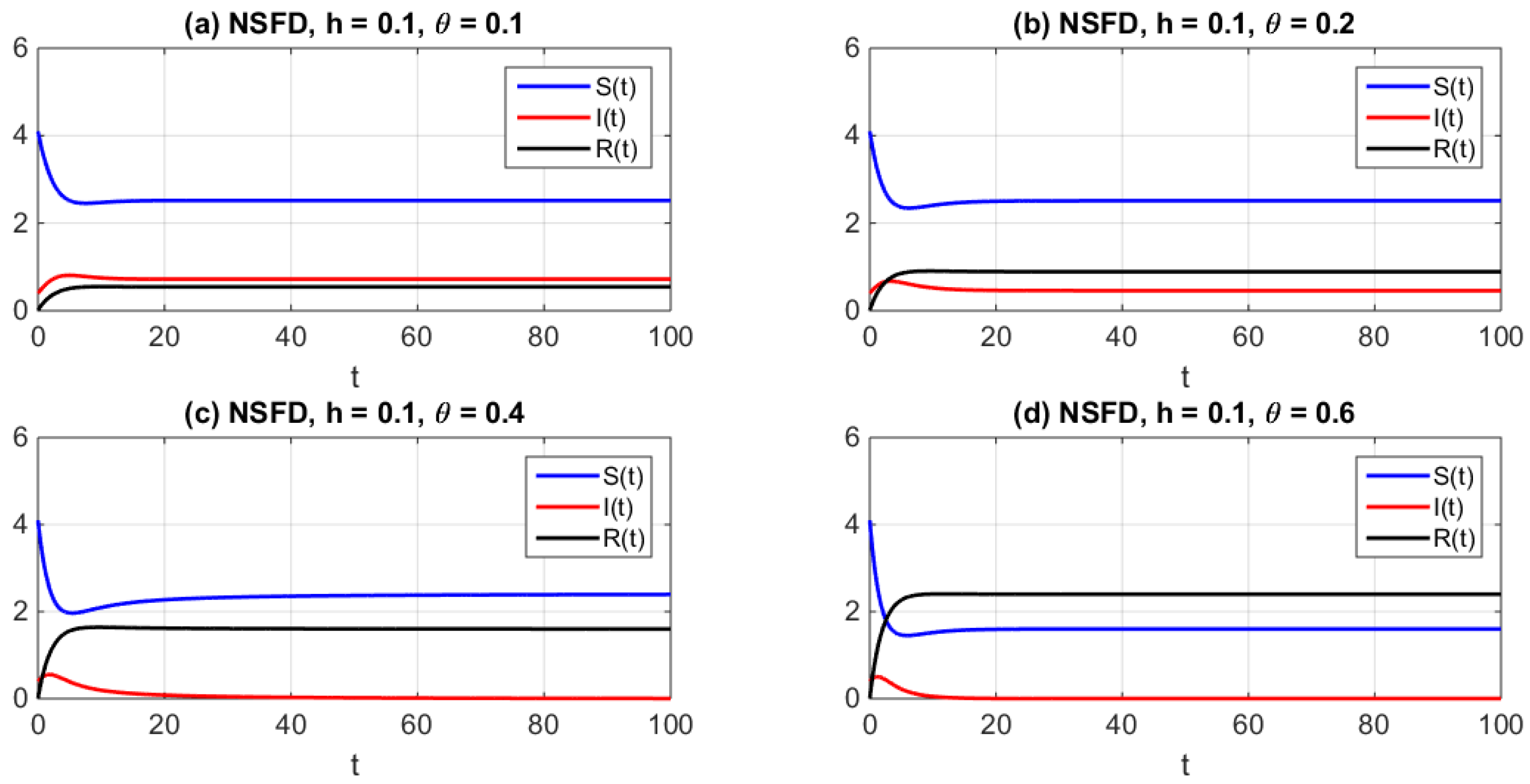
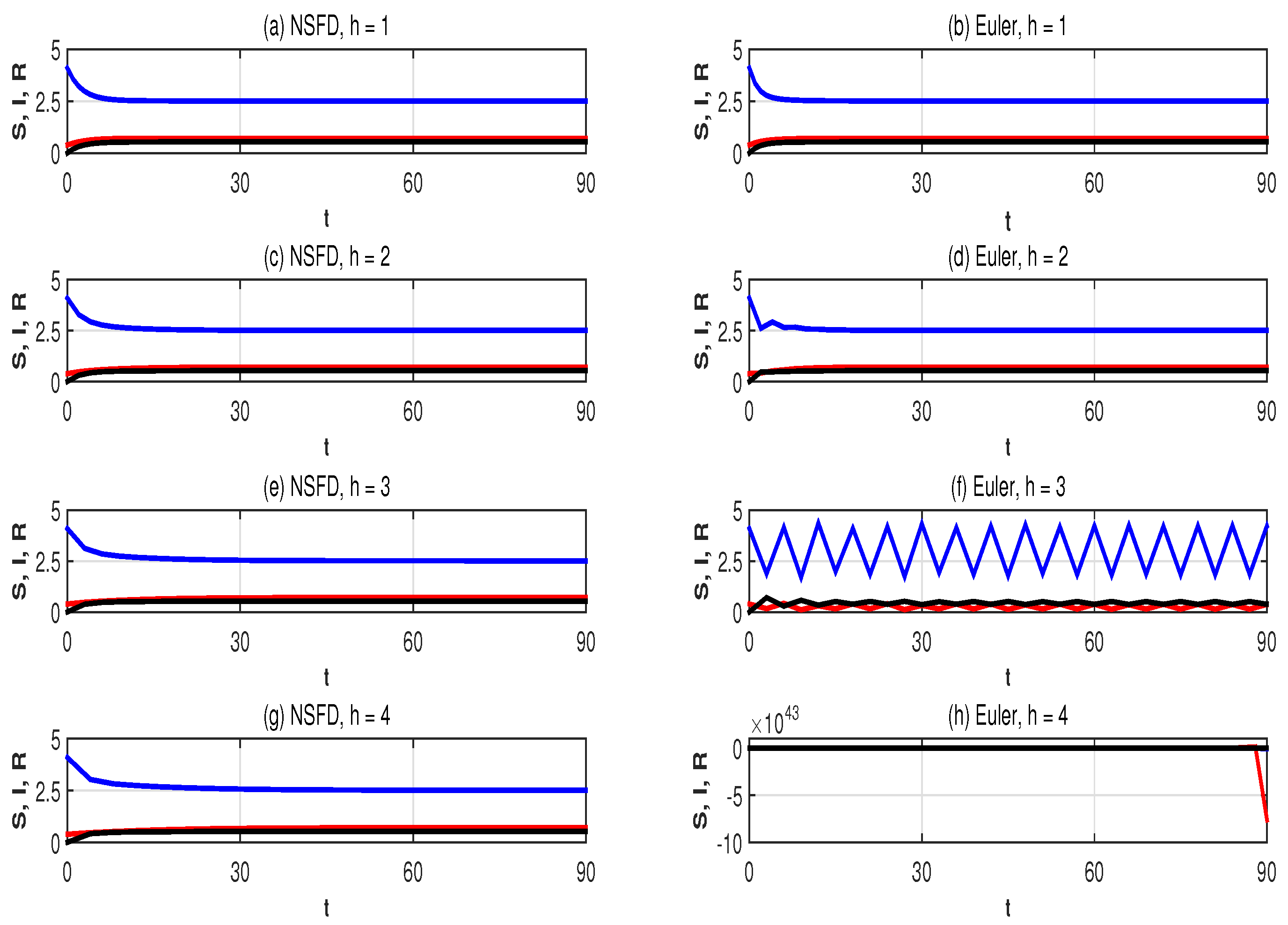
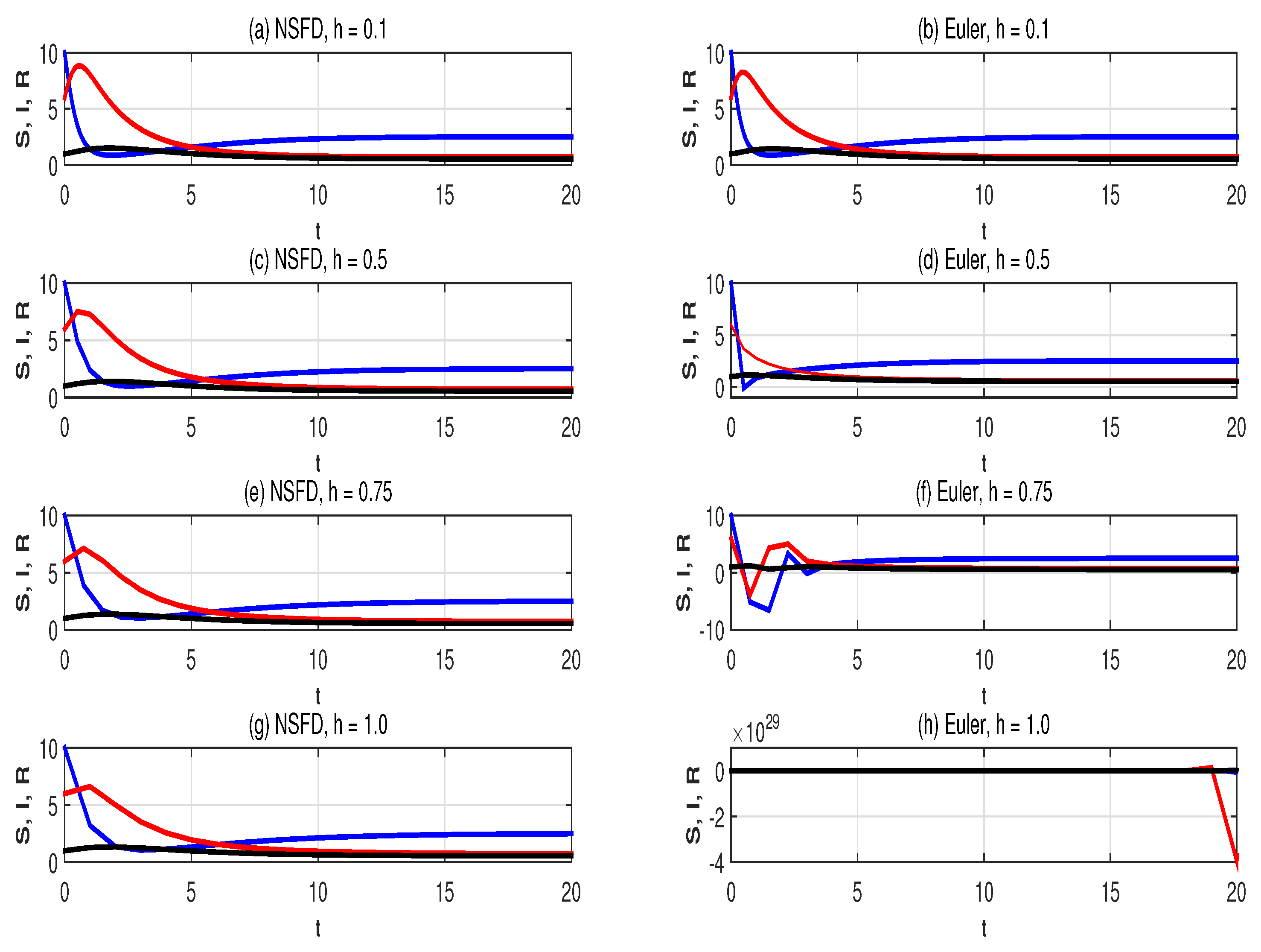
4. Numerical Simulations

To illustrate our previous analytical results, we provide some results of numerical simulations using hypothetical parameters: $A=2,$ $b=0.3,m=0.5,$ $a=0.01,$ $g=0.1$ and $e=0.15$. If we take $\theta =0.1,$ $0.2,$ $0.4$ and $0.6$ then the reproduction numbers of the model (1) are respectively ${\mathcal{R}}_0=1.44,$ $1.28,$ $0.96$ and $0.64$. Clearly that if we increase the constant of vaccination rate at birth ($\theta$) then the value of basic reproduction number ${\mathcal{R}}_0$ is reduced. From the previous section, we know that if ${\mathcal{R}}_0<1$ then the DFE point is globally asymptotically stable. On the other hand, ${\mathcal{R}}_0>0$ leads to the global stability of the EE point. Such dynamical behavior is confirmed by our numerical simulations using the NSFD scheme (9) with $h=0.1$; see Figure 2. The initial values for these simulations were $S\left(0\right)=4.1,I\left(0\right)=0.4$ and $R\left(0\right)=0.01$.

To see the influence of time-step size (h), we show in Figure 3 numerical solutions of model (1) with $\theta =0.1$ and initial value $S\left(0\right)=4.1,I\left(0\right)=0.4$ and $R\left(0\right)=0.01$ using different values of h. It is shown that all numerical solutions obtained by the proposed NSFD scheme (9) with $h=1,2,3,4$ are convergent to the EE point, showing that the stability of the EE point is independent of h. Such behavior cannot be achieved if we implement the explicit Euler scheme with a relatively large time-step size. Figure 3b,d shows that for relatively small h, the numerical solutions obtained by the explicit Euler scheme are also convergent to the EE point. However, the solution of the explicit Euler scheme with $h=3$ is convergent to a periodic solution of period-2, see Figure 3f. Moreover, the explicit Euler scheme with $h=4$ produces a divergent solution, see Figure 3h.

Finally, we performed numerical simulations using the same parameter values as in Figure 3 but with different initial values, namely, $S\left(0\right)=10,$ $I\left(0\right)=6$ and $R\left(0\right)=1$. We plotted numerical solutions obtained by the proposed NSFD scheme (9) and the explicit Euler scheme in Figure 4. This figure shows that the NSFD scheme gives non-negative solutions that are convergent to the correct equilibrium point. Although the solutions obtained by the explicit Euler scheme with $h=0.5$ and $h=0.75$ are also convergent to the correct equilibrium point, the solutions are biologically unrealistic because the solutions are negative at some points. The explicit Euler scheme with higher time-step sizes may also give a non-convergent solution; see Figure 4h. Figure 3 and Figure 4 confirm that the proposed NSFD scheme (9) is dynamically consistent with the model (1) regardless the value of h. On the contrary, the dynamical consistency of the explicit Euler scheme was achieved only for a relatively small h.

5. Conclusions

A SIR epidemic model of childhood diseases with a saturated incidence rate and constant vaccination strategy has been introduced. The non-negativity of the solutions and the conservation of population law for the proposed model have been shown. It is also shown that the model has always a DFE point which is (locally and globally) asymptotically stable if ${\mathcal{R}}_0<1$. If ${\mathcal{R}}_0>1$, then the DFE point is unstable and there appears an EE point, which is (locally and globally) asymptotically stable. In this paper, we have also proposed a discrete-time analog of the continuous childhood diseases epidemic model. To achieve this objective, we discretized the continuous model using the NSFD method. It is shown that the solutions of the constructed discrete NSFD model are always non-negative and satisfy the exact population conservation law. Furthermore, by verifying the eigenvalues of the Jacobian matrix of the proposed discrete NSFD model and taking suitable discrete Lyapunov functions, we have established the local and global stability for both DFE and EE points. Both the local and stability properties of the discrete NSFD model are exactly the same as those of the corresponding continuous model, which are entirely controlled by the basic reproduction number and do not depend on the time-step size. Hence, the proposed NSFD discrete model is dynamically consistent with the continuous SIR epidemic model of childhood diseases. The analytical results have been confirmed by our numerical simulations.

References

1. Makinde, O.D. Adomian decomposition approach to a SIR epidemic model with constant vaccination strategy. Appl. Math. Comput. 2007, 184, 842–848. [Google Scholar] [CrossRef]
2. Xu, R.; Ma, Z.; Wang, Z. Global stability of a delayed SIRS epidemic model with saturation incidence and temporary immunity. Comput. Math. Appl. 2010, 59, 3211–3221. [Google Scholar] [CrossRef] [Green Version]
3. Jana, S.; Nandi, S.K.; Kar, T.K. Complex Dynamics of an SIR Epidemic Model with Saturated Incidence Rate and Treatment. Acta Biotheor. 2016, 64, 65–84. [Google Scholar] [CrossRef] [PubMed]
4. Lashari, A.A. Optimal Control of an SIR Epidemic Model with a Saturated Treatment. Appl. Math. Inf. Sci. 2016, 10, 185–191. [Google Scholar] [CrossRef]
5. Ghosh, J.K.; Ghosh, U.; Biswas, M.H.A.; Sarkar, S. Qualitative Analysis and Optimal Control Strategy of an SIR Model with Saturated Incidence and Treatment. Differ. Equ. Dyn. Syst. 2019. [Google Scholar] [CrossRef] [Green Version]
6. Anderson, R.M.; May, R.M. Regulation and Stability of Host-Parasite Population Interactions: I. Regulatory Processes. J. Anim. Ecol. 1978, 47, 219–247. [Google Scholar] [CrossRef]
7. Yildirim, A.; Cherruault, Y. Analytical approximate solution of a SIR epidemic model with constant vaccination strategy by homotopy perturbation method. Differ. Equ. Dyn. Syst. 2009, 38, 1566–1575. [Google Scholar]
8. Mickens, R. Non Standard Finite Difference Models of Differential Equations; World Scientific: Singapore, 1994. [Google Scholar]
9. Darti, I.; Suryanto, A. Stability preserving non-standard finite difference scheme for a harvesting Leslie- Gower predator-prey model. J. Differ. Equ. Appl. 2015, 21, 528–534. [Google Scholar] [CrossRef]
10. Darti, I.; Suryanto, A. Dynamics preserving nonstandard finite difference method for the modified Leslie–Gower predator-prey model with Holling–type II functional response. Far East J. Math. Sci. 2016, 99, 719–733. [Google Scholar]
11. Rao, P.R.S.; Ratnam, K.V.; Murthy, M.S.R. Stability preserving non standard finite difference schemes for certain biological models. Int. J. Dyn. Control 2018, 6, 1496–1504. [Google Scholar]
12. Shabbir, M.S.; Din, M.S.; Khan, M.A.; Ahmad, K. A dynamically consistent nonstandard finite difference scheme for a predator–prey model. Adv. Differ. Equ. 2019, 2019, 381. [Google Scholar] [CrossRef] [Green Version]
13. Mickens, R.E. A SIR-model with square-root dynamics: An NSFD scheme. J. Differ. Equ. Appl. 2010, 16, 209–216. [Google Scholar] [CrossRef]
14. Garba, S.; Gumel, A.; Lubuma, J.S. Dynamically-consistent non-standard finite difference method for an epidemic model. Math. Comput. Model. 2011, 53, 131–150. [Google Scholar] [CrossRef]
15. Cui, Q.; Yang, X.; Zhang, Q. An NSFD scheme for a class of SIR epidemic models with vaccination and treatment. J. Differ. Equ. Appl. 2014, 20, 416–422. [Google Scholar] [CrossRef]
16. Cui, Q.; Zhang, Q. Global stability of a discrete SIR epidemic model with vaccination and treatment. J. Differ. Equ. Appl. 2015, 21, 111–117. [Google Scholar] [CrossRef]
17. Hattaf, K.; Lashari, A.A.; El Boukari, B.; Yousfi, N. Effect of discretization on dynamical behaviour in an epidemiological model. Differ. Equ. Dyn. Syst. 2015, 23, 403–413. [Google Scholar] [CrossRef]
18. Fitriah, Z.; Suryanto, A. Nonstandard finite difference scheme for SIRS epidemic model with disease-related death. AIP Conf. Proc. 2016, 1723, 030009. [Google Scholar]
19. Darti, I.; Suryanto, A.; Hartono, M. Global stability of a discrete SIR epidemic model with saturated incidence rate and death induced by the disease. Commun. Math. Biol. Neurosci. 2020, 2020, 33. [Google Scholar]
20. Cui, Q.; Xu, J.; Zhang, Q.; Wang, K. An NSFD scheme for SIR epidemic models of childhood diseases with constant vaccination strategy. Adv. Differ. Equ. 2014, 2014, 172. [Google Scholar] [CrossRef] [Green Version]
21. Mickens, R.E. Calculation of denominator functions for nonstandard finite difference schemes for differential equations satisfying a positivity condition. Numer. Methods Partial Differ. Equ. 2007, 23, 672–691. [Google Scholar] [CrossRef]
22. Brauer, F.; Castillo-Chavez, C. Mathematical Model in Population Biology and Epidemiology, 2nd ed.; Springer: New York, NY, USA, 2010. [Google Scholar]
23. Elaydi, S. An Introduction to Difference Equations, 3rd ed.; Springer: New York, NY, USA, 2005. [Google Scholar]
24. Enatsu, Y.; Nakata, Y.; Muroya, Y.; Izzo, G.; Vecchio, A. Global dynamics of difference equations for SIR epidemic models with a class of nonlinear incidence rates. J. Differ. Equ. Appl. 2012, 18, 1163–1181. [Google Scholar] [CrossRef] [Green Version]
Figure 1. Compartment diagram of the SIR epidemic model of childhood diseases with a saturated incidence rate and constant vaccination strategy.
Mathematics 08 01459 g001
Figure 2. Numerical solutions of model (1) obtained by the proposed NSFD scheme using h = 0.1 and (a) θ = 0.1 , (b) θ = 0.2 , (c) θ = 0.4 , (d) θ = 0.6 .
Mathematics 08 01459 g002
Figure 3. Numerical solutions of model (1) with θ = 0.1 obtained by the proposed NSFD scheme (left panels) and the explicit Euler scheme (right panels) for different values of time-step size (h). The initial values were S ( 0 ) = 4.1 ,   I ( 0 ) = 0.4 and R ( 0 ) = 0.01 .
Mathematics 08 01459 g003
Figure 4. Numerical solutions of model (1) with θ = 0.1 obtained by the proposed NSFD scheme (left panels) and the explicit Euler scheme (right panels) for different values of time-step size (h). The initial values were S ( 0 ) = 10 , I ( 0 ) = 6 and R ( 0 ) = 1 .
Mathematics 08 01459 g004