Inverse Minimum Cut Problem with Lower and Upper Bounds


Department of Mathematics and Computer Science, Faculty of Mathematics and Computer Science, Transilvania University of Brasov, 50003 Brașov, Romania
*
Author to whom correspondence should be addressed.
Mathematics 2020, 8(9), 1494; https://doi.org/10.3390/math8091494
Submission received: 23 July 2020
/
Revised: 30 August 2020
/
Accepted: 31 August 2020
/
Published: 3 September 2020
(This article belongs to the Special Issue Inverse and Ill-Posed Problems)
Abstract
:The inverse minimum cut problem is one of the classical inverse optimization researches. In this paper, the inverse minimum cut with a lower and upper bounds problem is considered. The problem is to change both, the lower and upper bounds on arcs so that a given feasible cut becomes a minimum cut in the modified network and the distance between the initial vector of bounds and the modified one is minimized. A strongly polynomial algorithm to solve the problem under norm is developed.
1. Introduction
Inverse optimization is a relatively new research domain (around 20 years old) and it has been intensively studied. Many papers have recently been published in this domain and are still being published nowadays. Inverse problems have lately found a lot of applications in modern areas, such as mathematical biology, materials science, remote sensing, medical imaging, seismology, geophysics, oceanography, mathematical finance, etc. An inverse combinatorial optimization problem consists of modifying some parameters of a network, such as capacities or costs, so that a given feasible solution of the direct optimization problem becomes an optimum solution and the distance between the initial vector and the modified vector of parameters is minimized. Different norms, such as , , and even , or Hamming distances are considered to measure this distance. In the last years, many papers were published in the field of inverse combinatorial optimization [1,2,3,4]. Among these problems, inverse maximum flow (IMF) and inverse minimum cut (IMC) problems were studied since their direct counterparts are well known related problems. Yang et al. [5] presented the first strong polynomial-time algorithms to solve these two problems under the norm. IMF is to change as little as possible the capacities of arcs so that a given feasible flow becomes optimum (maximum). IMF under was studied in [6]. Other IMF problems were studied in [7,8,9]. IMF considered for modification of upper and lower bounds on arcs was studied in [10] and it is the first time when both bounds are taken into account. The inverse minimum flow problem (ImF) was studied in [11]. In the case of IMC, the capacities (upper bounds) of arcs are changed, so that a cut becomes a minimum cut in the modified network. IMC is less studied than its related problem, IMF. Some inverse minimum cuts problems are considered in [12].
This paper studies the inverse minimum cut problem, where both lower and upper bounds on arcs are modified, so that the distance between initial vector of bounds and the vector of changed bounds measured with the norm is minimized and a given cut in the initial network becomes a minimum cut in the modified one. This problem is denoted as IMCUL. Although the direct problem of minimum cut with lower and upper bounds is a generalization of the problem of minimum cut with only upper bounds (where lower bounds can be considered equal to 0), the corresponding inverse problem IMCUL is a different problem and is not a generalization of IMC, since in the case of IMC lower bounds cannot be modified. Moreover, as we shall see in this paper, in comparison with [5], the methods used to solve these two inverse problems are completely different.
The rest of the paper is organized as follows. Section 2 presents the minimum cut and maximum flow with lower and upper bounds problems. Section 3 introduces the inverse minimum cut problem with lower and upper bounds (IMCUL) and a strongly polynomial algorithm to solve the IMCUL under the norm is also presented. In Section 4, an example is given to illustrate the idea of the proposed algorithm to solve IMCUL under the norm. Some conclusions are made and some open problems are presented in the last section.
2. Minimum Cut and Maximum Flow
Let be a network, where is the set of nodes, is the set of directed arcs (each arc from connects two nodes and from ), is the upper bound (capacity) application , is the lower bound application, and are two special nodes from . These two nodes are called source, respectively, sink. For an arc , and are the minimum and, respectively, the maximum amount of flow that can pass through arc from node to node . Of course, .
A feasible flow in the network is a function that satisfies simultaneously the conditions (1–4):
The value of flow is denoted by and defined as follows:
A maximum flow is a feasible flow in and among all feasible flows in it has the maximum value (see (5)).
Before presenting the definitions of the cut and of the capacity of a cut we introduce the following notations:
- -
- for two non-empty sets of nodes and from , denotes the set of arcs that connects nodes from with the nodes from , i.e., ;
- -
- for a function , we define .
For a non-empty set we denote . The set of arcs is called cut in network . If and then is called cut;
The capacity of the cut is denoted by and is defined in (6):
From now on through the paper we will refer to a cut as a cut.
We recall two theorems that connect (minimum) cuts with (maximum) flows (see [13]):
Theorem 1.
The value of a feasible flow in equals the value of the flow on a cut and does not exceed the value of this cut (see (7)).
Theorem 2.
The value of a minimum s − t cut in equals the value of a maximum flow in (see (8)).
3. The Inverse Minimum Cut Problem with Lower and Upper Bounds
Let be a network.
We denote by the concatenation of the vectors and (the components of are placed after the components of ). We call the bound vector of the network .
Let be a cut in network .
The set of for which is a cut in the corresponding network is denoted by and defined in (9):
The inverse minimum cut problem (IMCUL) is to change the bound vector so that the given cut becomes a minimum cut in and the distance between the initial bound vector and the modified vector of bounds denoted is minimized (see (10)):
We shall concentrate now on the inverse minimum cut problem with lower and upper bounds under the norm (denoted IMCUL1). More exactly, for IMCUL the distance between and is measured using the norm. This means that the sum of absolute modifications of the bounds on arcs is minimized (see (11a)):
We recall the definition of norm for the -dimensional vector :
Lemma 1.
If is the optimum solution of IMCUL1 then we have:
Proof.
Let us suppose that one of the relations (12a) or (12b) is false. This means that there exists an arc so that or so that .
We define a capacity vector as follows:
It is easy to observe that (see (13)) and
Relation (14) contradicts the optimality of .
Let us suppose now that one of the relations (12c) or (12d) is false. This means that there exists an arc so that or so that .
We define the following lower bound vector :
It is easy to observe that (see (15)) and
Relation (14) contradicts the optimality of . □
Lemma 2.
- (a)
- If the capacity of an arc is increased with the value then the difference between the value of the maximum flow in the modified network and the value of the maximum flow in the initial network is not greater than .
- (b)
- If the lower bound of an arc is decreased with the value then the difference between the value of the maximum flow in the modified network and the value of the maximum flow in the initial network is not greater than .
Proof.
Let us consider a maximum flow in the network and a minimum cut in .
(a) After the capacity of the arc is increased with the value , the capacity vector is obtained in (17):
Let be a maximum flow in the modified network . It is easy to observe that the existence of a feasible flow (and a maximum flow) in is assured by the fact that and by the existence of a maximum flow in .
Of course, we have two possible situations: The arc is in the direct set of arcs of a minimum cut in or not.
Case a.1. There is a minimum cut in so that the arc .
Let be a minimum cut in . It is easy to see that:
Case a.2. There is no minimum cut in so that the arc .
Let be a minimum cut in . Of course, . We shall prove next that is a minimum cut in .
Let be a cut in . It follows that (if ) and (if ). Therefore, and, since ( and is a minimum cut in ), it results that . It follows that is the minimum cut in because is the arbitrarily chosen cut in .
Since is a minimum cut in both networks, and , and it results in equality (19):
Therefore, in both cases, relation (20) was obtained:
(b) After the lower bound of the arc is decreased with the value , the following lower bound vector is obtained in (21):
A modified network is considered now and is a maximum flow in . The existence of a feasible flow (and a maximum flow) in is assured by the fact that and by the existence of a maximum flow in .
We have two possible situations: The arc is in the inverse set of arcs of a minimum cut in or not.
Case b.1. There is a minimum cut in so that the arc .
Let be a minimum cut in . It is easy to see that:
Case b.2. There is no minimum cut in so that the arc .
Let be a minimum cut in . Of course, . We shall prove next that is a minimum cut in .
Let be a cut in . It follows that (if ) or (if ). Therefore, and, since ( and is a minimum cut in ), it results that . It follows that is the minimum cut in because is the arbitrarily chosen cut in .
Since is a minimum cut in both networks, and , and it results in equality (23):
Therefore, in both cases, b.1 and b.2, relation (24) was obtained:
□
Theorem 3.
The pair of vectors given in (25) and (26) is the optimum solution of IMCUL1, where:
Proof.
Let be an optimum solution of IMCUL1. A maximum flow is considered in the network .
Using Lemma 1 and from the fact that is an optimum solution of IMCUL1 the relations from (27) are obtained:
Therefore, if the upper bounds on arcs or the lower bounds of are modified then the value of the maximum flow is increased. Using Lemma 2 it results that:
Using Lemma 1 it follows that:
Using the definition of and (see (25) and (26)) we have:
From (29) and (30) it results that:
Using the definition of and (see (25) and (26)) we have:
From this equality and from the fact that is a feasible flow in it results that is the minimum cut in and the feasible solution of IMCUL1. It results that:
This means that is an optimum solution of IMCUL1. □
Corollary 1.
If is an optimum solution of IMCUL1, then the distance between and the initial vector is given in (33):
Proof.
It is directly from (30) and (32). □
Corollary 2.
If is an optimum solution of IMCUL1, it is given in (34):
Proof.
Using Corollary 1, inequality (29) becomes equality and then inequality (28) becomes also an equality. □
From Theorem 3 the following algorithm denoted AIMCUL1 is obtained to solve IMCUL1:
- AIMCUL1
- Calculate a maximum flow in ;
- Using (25) and (26) construct ;
- is an optimum solution of IMCUL1.
The maximum flow problem has been intensively studied over decades [13]. A lot of algorithms to solve it have been developed. The first algorithm was proposed by Ford and Fulkerson in 1956. As long as there is an augmenting path in the network, the flow is increased along this path. This algorithm is not polynomial since its time complexity linearly depends on the value of the maximum flow. However, it is the base idea for other algorithms such as those due to Edmonds-Karp or Dinic which are polynomial (the time complexity is polynomial in the number of nodes and the number of arcs). There are also other polynomial approaches based on maintaining a preflow (push-relabel maximum flow). The best current known algorithm was published in 2013 by James Orlin [14]. This algorithm solves the maximum flow problem as a sequence of improvement phases. A strongly polynomial time algorithm was obtained by replacing the residual network of the Δ-improvement phase by a more compact representation. The author proved that the maximum flow can be computed in time or even if , where n is the number of nodes () and m is the number of arcs ().
Theorem 4.
The time complexity of AIMCUL1 is .
Proof.
The time complexity of AIMCUL1 is given by the time complexity of the algorithm used to calculate the maximum flow . □
4. Example
We shall give an example to illustrate how AIMCUL1 works. In Figure 1, a network G and a given s − t cut in G are presented. The maximum flow is calculated in G (see Figure 2) using any known algorithm briefly presented before theorem 4. The optimum solution is presented in Figure 3. The upper bounds of the arcs (3, 6) and (7, 6) were modified from 6 to 5 and, respectively, from 3 to 1 according to formula (25). The lower bound of the arc (2, 3) was modified from 1 to 3 using formula (26). The total amount of modifications brought to the boundaries is (6 − 5) + (3 − 1) + (3 − 1) = 5. Therefore, becomes a minimum s − t cut in .
5. Conclusions
An efficient strongly polynomial algorithm was deduced to solve IMCUL1. Although the direct problem of minimum cut with lower and upper bounds is a generalization of the problem of minimum cut with only upper bounds, the corresponding inverse problem IMCUL1 is a different problem, which is not a generalization of IMC since in the case of IMC lower bounds cannot be modified. An example to illustrate the proposed algorithm for IMCUL1 has been presented.
As a future work, the inverse minimum cut with lower and upper bounds under other norms and distances (such as , or Hamming distances) could be considered.
Author Contributions
Conceptualization, A.D.; methodology, L.C.; validation, L.C.; formal analysis, A.D.; writing—original draft preparation, A.D.; writing—review and editing, L.C. and A.D.; funding acquisition, A.D. and L.C. All authors have read and agreed to the published version of the manuscript.
Funding
The APC was funded by Transilvania University of Brasov.
Conflicts of Interest
The authors declare no conflict of interest.
References
- Ahuja, R.K.; Orlin, J.B. Combinatorial algorithms for inverse network flow problems. Networks 2002, 40, 181–187. [Google Scholar] [CrossRef] [Green Version]
- Ahuja, R.K.; Orlin, J.B. Inverse Optimization. Oper. Res. 2001, 49, 771–783. [Google Scholar] [CrossRef]
- Demange, M.; Monnot, J. An introduction to inverse combinatorial problems. In Vangelis Th. Paschos, Paradigms of Combinatorial Optimization (Problems and New Approaches); Wiley: London, UK; Hoboken, NJ, USA, 2010. [Google Scholar]
- Heuberger, C. Inverse Combinatorial Optimization: A Survey on Problems, Methods, and Results. J. Comb. Optim. 2004, 8, 329–361. [Google Scholar] [CrossRef] [Green Version]
- Yang, C.; Zhang, J.; Ma, Z. Inverse maximum flow and minimum cut problems. Optimization 1997, 40, 147–170. [Google Scholar] [CrossRef]
- Deaconu, A. The inverse maximum flow problem considering L∞ norm. RAIRO Oper. Res. 2008, 42, 401–414. [Google Scholar] [CrossRef]
- Tayyebi, J.; Deaconu, A. Inverse Generalized Maximum Flow Problems. Mathematics 2019, 7, 899. [Google Scholar] [CrossRef] [Green Version]
- Tayyebi, J.; Mohammadi, A.; Kazemi, S.M.R. Reverse maximum flow problem under the weighted Chebyshev distance. RAIRO Oper. Res. 2018, 52, 1107–1121. [Google Scholar] [CrossRef]
- Liu, L.; Zhang, J. Inverse maximum flow problems under the weighted Hamming distance. J. Comb. Optim. 2006, 12, 395–408. [Google Scholar] [CrossRef]
- Deaconu, A. The inverse maximum flow problem with lower and upper bounds for the flow. Yugosl. J. Oper. Res. 2008, 18, 13–22. [Google Scholar] [CrossRef]
- Ciurea, E.; Deaconu, A. Inverse minimum flow problem. J. Appl. Math. Comput. 2007, 23, 193–203. [Google Scholar] [CrossRef]
- Zhang, J.; Cai, M.-C. Inverse problem of minimum cuts. ZOR-Math. Methods Oper. Res. 1998, 47, 51–58. [Google Scholar] [CrossRef]
- Smith, D.K.; Ahuja, R.K.; Magnanti, T.L.; Orlin, J.B. Network Flows: Theory, Algorithms, and Applications; Prentice Hall: Englewood Cliffs, NJ, USA, 1993. [Google Scholar]
- Orlin, J.B. Max flows in O(nm) time, or better. In Proceedings of the Forty-fifth Annual ACM Symposium on Theory of Computing, Palo Alto, CA, USA, 2–4 June 2013; pp. 765–774. [Google Scholar]
Figure 1.
Initial network G and s − t cut .
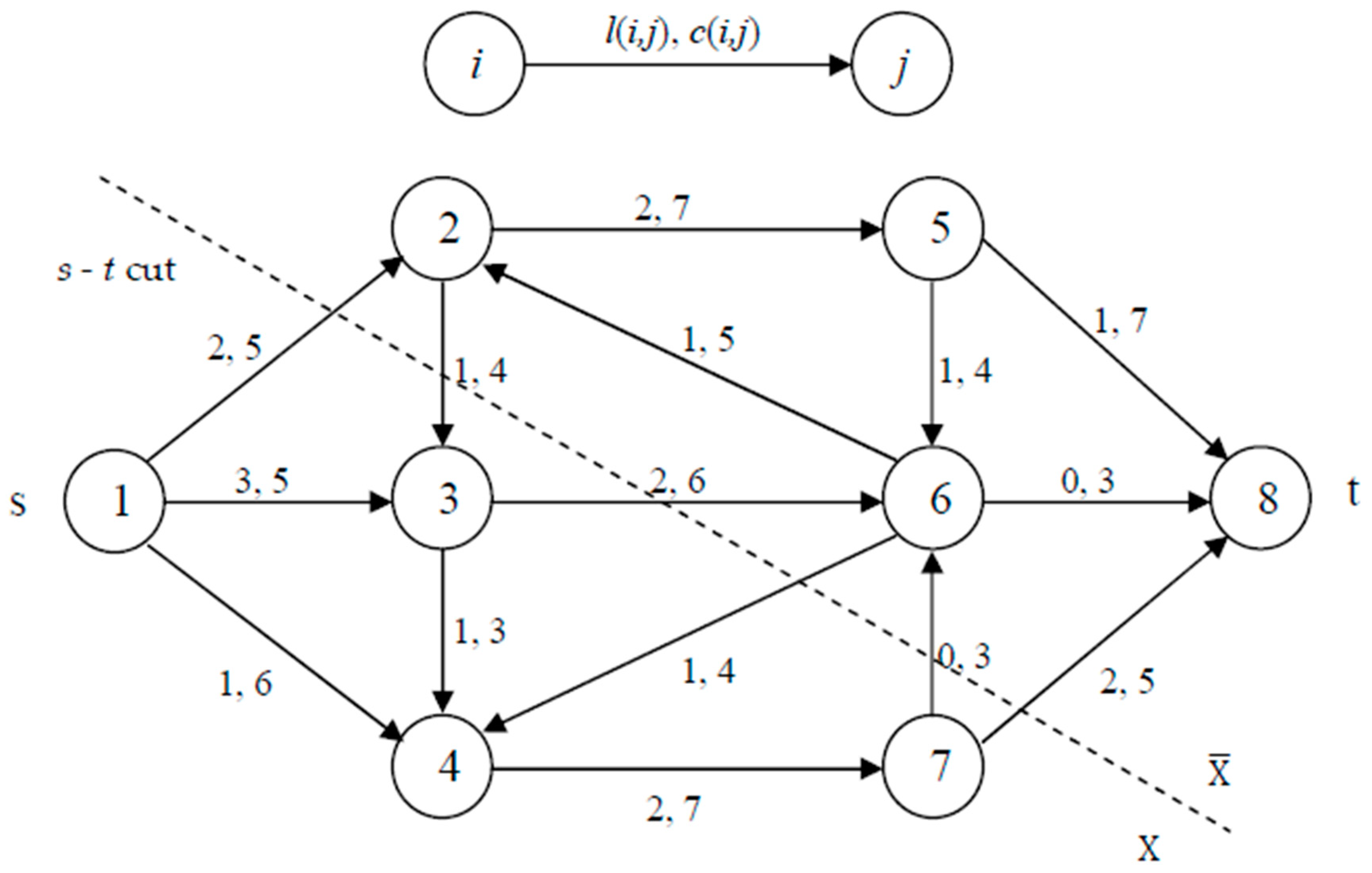
Figure 2.
Maximum flow in G.

Figure 3.
Optimum solution of inverse minimum cut problem with lower and upper bounds 1 (IMCUL1).

© 2020 by the authors. Licensee MDPI, Basel, Switzerland. This article is an open access article distributed under the terms and conditions of the Creative Commons Attribution (CC BY) license (http://creativecommons.org/licenses/by/4.0/).
Share and Cite
MDPI and ACS Style
Deaconu, A.; Ciupala, L. Inverse Minimum Cut Problem with Lower and Upper Bounds. Mathematics 2020, 8, 1494. https://doi.org/10.3390/math8091494
AMA Style
Deaconu A, Ciupala L. Inverse Minimum Cut Problem with Lower and Upper Bounds. Mathematics. 2020; 8(9):1494. https://doi.org/10.3390/math8091494
Chicago/Turabian StyleDeaconu, Adrian, and Laura Ciupala. 2020. "Inverse Minimum Cut Problem with Lower and Upper Bounds" Mathematics 8, no. 9: 1494. https://doi.org/10.3390/math8091494
Note that from the first issue of 2016, this journal uses article numbers instead of page numbers. See further details here.