Abstract
We investigate why normal electrons in superconductors have no resistance. Under the same conditions, the band gap is reduced to zero as well, but normal electrons at superconducting states are condensed into this virtual energy band gap.
1. Introduction
The conventional properties of superconductors different from normal materials are classified as no resistance below a critical temperature and no magnetic field inside bulk. Following the discovery of superconductivity by Onnes [1], the phenomenon could be described quite well for low temperatures by Bardeen–Cooper–Schrieffer (BCS) theory [2]. The mechanism was derived from electron–electron interactions mediated by lattice ions where this indirect interaction exceeds direct Coulomb interaction, such that the repulsive Coulomb interaction is overcome, thereby causing attraction to occur. Ionic intervention was therefore confirmed to be the experimental observation of the isotope effect, providing strong evidence in support of the BCS model. In contrast, the discovery in 1986 of high-temperature superconductivity [3] has not yet been fully accepted and acknowledged by theoreticians, and debates about this have been introduced [4,5]. However, many theoretical models have been proposed [6,7]. One important characteristic of high-temperature superconductors (HTSCs) is the existence of CuO2 planes in their structures. However, the linear dependence of resistivity on temperature, the very high superconducting transition temperatures, and the origin of the pseudo-gap, among other things, all still require clearer explanations if a full consensus is to be achieved on a theoretical model for HTSCs. Some theoretical approaches to HTSCs are still under development, in a Heisenberg antiferromagnetic model [8] that uses the formalism of Green’s function and in the attractive Hubbard model [9], which makes use of dynamical mean field theory. Poor metals comprise most low-temperature superconductors, while it is doping in insulators that is found to explain most high-temperature ones. As shown by McMillan [10], strong interactions can give rise to low-temperature superconductors up to a maximum highest superconducting transition temperature of around 30 K. Therefore, for high-temperature superconductors with transition temperatures above 40 K, we generally require either a restructured BCS theory or a different theoretical basis altogether. Furthermore, for superconductors in general, we have no clear explanation of why the remaining normal electrons show no resistance. Although we are satisfied with the assumption itself, the superconducting electrons and the normal-state electrons of finite resistance act in a parallel circuit connection to make the total resistance of the circuit tend to zero [11,12]. This postulate has not yet been confirmed. Conventional theories calculate band gaps by applying a model with standing wave-like wave functions, either by applying Bragg diffraction or another scheme that makes use of periodic Bloch wave equations [13,14].
In the present work, under a mean-field scheme, we calculate the band gaps using an analogy with the BCS scheme for the calculation of superconducting gaps. We can also explain the reason for the lack of resistance of normal electrons in initial superconducting states, matching with band gaps. Because original BCS theory adopted a mean-field approach, we can solve the no-resistance problem within this scheme. The rest of the paper is organised as follows. Section 2 contains the basic equations. Section 3 contains the results and discussions. Section 4 contains the conclusions.
2. Model and Basic Equations
We first consider superconductors.
The BCS-type Hamiltonian [15] for low-temperature superconductors is given by
where the BCS-type electron–electron interaction is given by
In the above equations, is the phonon energy, is the coupling constant of electron–phonon interactions, designates the spin states of the electrons, is the electron kinetic energy, is an annihilation operator, and is the Coulomb interaction.
The reduced BCS-type Hamiltonian becomes
when used with the BCS approach, in which the brackets < > denote the average of the mean field.
Using the Bogoliubov transformation [15], the operators are given by
where the operator, corresponds to a quasiparticle composed of an electron with amplitude and a hole with amplitude .
The gap equation is given by
Using the above equations for normal materials, the resulting superconducting gap and band gap are given by
where is the phonon energy; is the density of the states at the Fermi level, which is changed into the real value of ; and is the band gap, and the imaginary part is for the real part of with a phase angle of . If is nonzero, Equation (6) cannot be singular [16]. Either the superconducting gap or the band gap must be zero, so they cannot coexist. In Equation (2), the denominator can be positive in the case of inter-band interactions between copper (Cu) and oxygen (O) but negative for intra-band ones for cuprate superconductors. For band gaps, the situation is the same, except for inter-band interactions between the conduction band and valence band.
The large band gap is independent of temperature, in agreement with experimental data [13,14]. The temperature dependence that we find for small band gaps may afford a better interpretation of the experimental data [13,14].
The gap equation under the postulate of Bose–Einstein condensations is given by
is the Bose–Einstein distribution function, and the Bose–Einstein gap is given as
Here, we interpret this to mean that the normal-state band gap becomes zero in BCS superconductors and the Bose–Einstein condensation of the superconducting electrons is proportional to the virtual energy band gap that remains with normal electrons.
3. Results and Discussions
3.1. Criterion on Occurrence of Superconductivity
Let us consider the criterion on the occurrence of superconductivity in good metals.
At T = 0 K, the number of electrons across the Fermi energy [2] is given by
and the band gap at T = 0 K from Equation (6) is given as
and then the occurrence condition is obtained as
In silver and gold, good metals, the resultant attractive electron–electron interaction can be too strong to cover the bandgap, which is transformed into the condensation coverage at low temperatures, so no superconducting states occur. This fact contradicts the conventional belief that in good metals, the resultant electron–electron interactions may be repulsive or timidly attractive.
Now, we calculate the heat capacity for interacting electrons in silver (Ag).
From the Stoner theory [17], it is given as
where is the kinetic energy, is the Bohr magneton, is the magnetic field, is the Fermi energy, is the spin index, and is the transition temperature.
The heat capacity at constant volume, Cv, of silver crystal is calculated as
where it is assumed , is the Fermi-Dirac distribution, is the gas constant given as ( = 6.022 × 10²³ mol−1 is the Avogadro’s number and = 1.381 × 10⁻²³ J K−1 mol−1 is the Boltzmann constant), and is the delta function where the density of states centered at the Fermi level are postulated to be maximized. As shown in Figure 1, the molar heat capacity at constant volume, Cv, fits with the experimental molar heat capacity at constant pressure, Cp [18,19,20], of bulk silver, which crystallizes in a face-centered cubic (fcc) structure (space group Fm3m) and has a melting point of 962 °C [21].
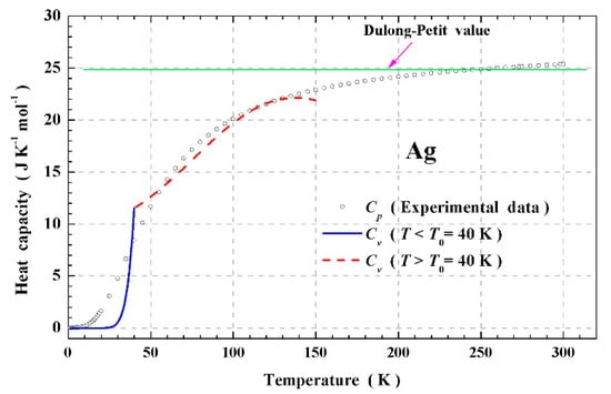
Figure 1.
The experimental molar heat capacity at constant pressure, Cp, [18,19,20] of bulk silver crystal fits with the theoretical molar heat capacity at constant volume, Cv, where the parameters are given for convenience as: ; ; .
To date, Josephson junctions in momentum space have not been fully investigated. This pseudo-Josephson junction model is appropriate for currents.
The experimental data were taken from [18,19,20] in the temperature range from 1 to 300 K. We used the conversion factor of gas constant = 8.314 J K−1 mol−1, where = 6.022 × 10²³ mol−1 is Avogadro’s number and = 1.381 × 10⁻²³ J K−1 mol−1 is the Boltzmann constant. The Cp value approaches the classical Dulong–Petit value 3NAkB = 24.94 J K−1 mol−1 [14,15,20] as the temperature approaches 250 K, above which Cp exceeds the classical value due to the lattice anharmonic contributions in the potential energy. The open circles represent the experimental molar heat capacity, while the blue solid and the red dashed lines denote the calculated ones below and above the possible phase-transition temperature (To = 40 K) in Equation (13), respectively. Our analysis of the data may support the possibility of superconducting silver.
We first consider the pseudo-Josephson effect on the direct current. Let be the probability amplitude of electrons in the conduction band on one side of a junction (the band gap) and let be the probability amplitude on the valence electron band; the time-dependent Schrödinger equation applied to the two amplitudes gives
Here, represents the effect of transfer interaction across the band gap along the axis of energy: , where is the external voltage and is the energy gap of silver.
For the insulator with thickness longer than the superconducting coherence length under the maintenance of two superconductors [6,7], the current is contributed by the intercalated insulator and superconductors as
where are the amplitudes of the superconducting current density and the normal one; , N(0) is the density of state at Fermi level; is the Debye energy; is superconducting gap; is band gap from the intercalated insulator; and is the Fermi velocity. The number densities are given as
In order to unify the phases in Equation (15), it becomes
The effective band gap is determined as
From the viewpoint of physics, the effective bandgap is given as
This is approximated as
If we fabricate silver–insulator–silver as a Josephson-like junction, the superconductivity may occur at low temperatures. The effective band gap of silver is changed into
Other good metals also have the same cases. According to our conjectures, good metals including Ag, Cu, Au, and Pt can become superconducting as the band gaps increase.
Real superconducting states begin below the cusp resistivity region, just above the conventional superconducting temperature. Then, in this region, a Josephson-like tunneling between superconducting electrons via the insulating band gap is dominant in resistivity. The electrical resistivity just above the superconducting temperature and below the cusp is given as the reciprocal of the electrical conductivity :
where is from diamagnetic contributions and is given from a Matsubara relation [19].
3.2. Composite Charge
We applied the concept of an electric vortex first introduced for quark confinement [21], in which the vortex consisted of a local timid spatial pocket occupied by bundles of electric field lines. The effective charge of an electron attached to an electric flux is called a composite charge as shown in Figure 2 and expressed in Equation (23).
where is the effective charge; are the electric field and the surface in a portion of the bulk material (in an electric cylindrical vortex), respectively; is the electric permittivity inside the material; is the number of electric field lines in an electric vortex attached to an electron; is the total charge in a portion of the bulk material; are positive integers; and is a small integer representing electron and ion cancellations.
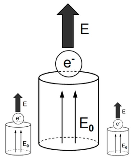
Figure 2.
An electron attached to an electric vortex.
From Gauss’s law for electricity,
becomes
We reinforce the mathematical background of the composite charges as follows.
For a charge q attached by a cylindrical vortex with z-directional electric fields and a cross surface of , from the Ampere–Maxwell law [22,23], we obtained the following:
where is a relationship between magnetic induction and a magnetic field .
The angular momentum is given by the Lorentz force as
The effective charge (the composite charge) is given by
Zero Coulomb repulsions can originate from the Nambu massive mode [24,25] or the Nambu holon [26,27], which is also termed the “Nambuon”, where spontaneous symmetry breaking occurs.
Candidates for the Nambuon are:
- (i)
- Two-dimensional elementary excitations.
- (ii)
- A spherically isotropic distributed mode, thus yielding = 1 and e* = 0e, −2e having zero Coulomb repulsions.
Since the electric field on the metallic plate [23] is , the value of becomes 1.
For spherically isotropic modes, , where is the effective radius.
Gauge invariance [26,27,28,29,30,31] in superconductors can be terminated because
where is the positive adjustable number of gauge electric field lines in an electric vortex attached to an electron. According to Schafroth [29], the BCS Hamiltonian and the current density operator are
where is an interaction dependent on coordinates and momenta , is the mass of an electron, is the velocity of light, is the delta function, and is the vector potential. To conserve gauge invariance, the following condition must be satisfied:
In our case, the bare charge is changed into effective charge in order to be gauge invariant in the presence of gauge fields. Therefore, our composite charge concepts can solve the long-standing paradox of gauge invariance in BCS theory.
4. Conclusions
In conclusion, band gaps originate from phonon-mediated BCS-type repulsive electron–electron interactions and Coulomb repulsions. If , the superconducting gap becomes zero, even though the band gap is nonzero. Non-crystalline amorphous silicon has a band gap, which contradicts the conventional belief that band gaps are induced by crystalline periodic potential. Even good conductors have a negligibly small bandgap in our model. Figure 3 illustrates that the band gap tends to zero in the superconducting state when the Bose–Einstein condensation is found to replace the virtual energy band gap. In terms of the Fermi surface diagrams, the normal-state electrons above the Fermi energy level in the superconducting system descend towards the band gap to fill the energy levels from zero up to the Fermi level, thereby forming a superconducting gap above the Fermi level to bring about the resistance-free state. According to our theory, Bose–Einstein condensation is established only up to the remaining virtual energy band gap; i.e., in the absence of a finite band gap energy associated with normal-state electrons, no superconducting condensation should be possible. Furthermore, with a slight doping of large-band-gap materials as in high-temperature superconductors, a large amount of superconducting condensation in proportion to the energy band gap may be possible at the transition temperature, making it possible to obtain high Tc superconductors [32,33]. In Equation (2), the denominator can be positive in the case of inter-band interactions between copper (Cu) and oxygen (O) in cuprate superconductors but negative for intra-band ones. For band gaps, the situation is same except for inter-band interactions between the conduction band and valence band. In silver and gold, good metals, the resultant attractive electron–electron interaction can be too strong to cover the bandgap, which is transformed into the condensation coverage at low temperatures, so no superconducting states occur. This fact contradicts the conventional belief that in good metals, the resultant electron–electron interactions may be repulsive or timidly attractive. As shown in Figure 1, the resultant electron–electron interactions of silver are repulsive above around 40 K and become strongly attractive below the temperature, so no superconductivity occurs. Long-standing overestimated large Coulomb repulsions ~5 eV can be resolved by obtaining zero values in superconductors. Long-standing debates about superconductivity have been introduced [4,5].
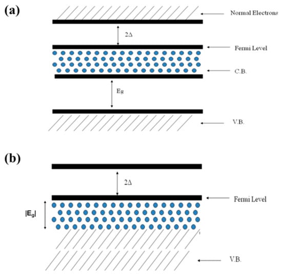
Figure 3.
The band gap Eg and the superconducting gap 2Δ are shown, where C.B. and V.B. denote the conduction band and the valence band, respectively: (a) at superconducting states according to conventional models; (b) at superconducting states according to our model.
Author Contributions
Conceptualization, C.S. and J.H.K.; methodology, J.H.K.; validation, C.S., S.C. and J.H.K.; formal analysis, J.H.K.; investigation, S.C.; writing—original draft preparation, C.S.; writing—review and editing, S.C. and J.H.K.; visualization, S.C.; supervision, J.H.K.; project administration, C.S.; funding acquisition, C.S. All authors have read and agreed to the published version of the manuscript.
Funding
This research received no external funding.
Acknowledgments
The work was supported by the Kongju National University, Gongju, Korea. (No. 2020-0296-01). The present research was conducted with funding from a Research Grant from Kwangwoon University in 2020.
Conflicts of Interest
The authors declare no conflict of interest.
References
- Schrieffer, J.R. Theory of Superconductivity; Benjamin: New York, NY, USA, 1964. [Google Scholar]
- Bardeen, J.; Cooper, L.N.; Schrieffer, J.R. Theory of Superconductivity. Phys. Rev. 1957, 108, 1175–1204. [Google Scholar] [CrossRef]
- Bednorz, J.G.; Muller, K.A. Possible High Tc Superconductivity in the Ba-La-Cu-O System. Z. Phys. B Condens. Matter. 1986, 64, 189–193. [Google Scholar] [CrossRef]
- Poole, C.P.; Farach, H.A.; Creswick, R.J.; Prozorov, R. Superconductivity; Elsevier: New York, NY, USA, 2007. [Google Scholar]
- Rose-Innes, A.C.; Rhoderick, E.H. Introduction to Superconductivity; Pergamon: New York, NY, USA, 1993. [Google Scholar]
- Koo, J.H.; Kim, J.H.; Jeong, J.M.; Cho, G.; Kim, J.J. Anomalous Spin Density Wave Superconductivity in Cuprate High-Tc Superconductors. Mod. Phys. Lett. B 2009, 23, 1533–1538. [Google Scholar] [CrossRef]
- Anderson, P.W. The resonating valence bond state in La2CuO4 and superconductivity. Science 1987, 235, 1196–1198. [Google Scholar] [CrossRef] [PubMed]
- de Sousa, J.R.; Pacobahyba, J.T.M.; Singh, M. A theoretical study of the extinction of antiferromagnetic order by holes and dilution in La1-xSrxCu1-zZnzO4. Solid State Commun. 2009, 149, 131–135. [Google Scholar] [CrossRef]
- Bauer, J.; Hewson, A.C.; Dupuis, N. Dynamical mean-field theory and numerical renormalization group study of superconductivity in the attractive Hubbard model. Phys. Rev. B 2009, 79, 214518. [Google Scholar] [CrossRef]
- McMillan, W.L. Transition temperature of strong-coupled superconductors. Phys. Rev. 1968, 167, 331. [Google Scholar] [CrossRef]
- Mourachkine, A. Room-Temperature Superconductivity; Cambridge Int Science Publishing: Cambridge, UK, 2004. [Google Scholar]
- Halperin, B.I.; Refael, G.; Demler, E. BCS: 50 Years; Cooper, L.N., Feldman, D., Eds.; World Scientific: Singapore, 2011; pp. 185–226. [Google Scholar]
- Kittel, C.; McEuen, P. Introduction to Solid State Physics; Wiley: New York, NY, USA, 1976; Volume 8. [Google Scholar]
- Ashcroft, N.W.; Mermin, N.D. Solid State Physics; Brooks/Cole: Pacific Grove, CA, USA, 1976. [Google Scholar]
- White, R.M.; Geballe, T.H.; Sak, J. Long Range Order in Solids. Phys. Today 1980, 33, 60. [Google Scholar] [CrossRef]
- Jewett, J.W.; Serway, R.A. Physics for Scientists and Engineers with Modern Physic; Brooks Cole: Singapore, 2010. [Google Scholar]
- Kim, D.J. New Perspectives in Magnetism of Metals; Springer Science & Business Media: Berlin, Germany, 1999. [Google Scholar]
- Touloukian, Y.S.; Buyco, E.H. Specific Heat. In Thermophysical Properties of Matter; IFI/Plenum: New York, NY, USA, 1970; Volume 4. [Google Scholar]
- Smith, D.R.; Fickett, F.R. Low-temperature properties of silver. J. Res. Natl. Inst. Stand. Technol. 1995, 100, 119. [Google Scholar] [CrossRef] [PubMed]
- Fegley, B., Jr. Practical Chemical Thermodynamics for Geoscientists; Academic Press: Cambridge, MA, USA, 2012. [Google Scholar]
- Nielsen, N.K.; Olesen, P. Electric vortex lines from the Yang-Mills theory. Phys. Lett. B 1978, 79, 304–308. [Google Scholar] [CrossRef]
- Gasiorowicz, S. Quantum Physics; John Wiley & Sons: New York, NY, USA, 1974. [Google Scholar]
- Purcell, E.M. Berkeley Physics Course: Electricity and Magnetism; McGraw-Hill: New York, NY, USA, 1985. [Google Scholar]
- Nambu, Y. Axial vector current conservation in weak interactions. Phys. Rev. Lett. 1960, 4, 380. [Google Scholar] [CrossRef]
- Nambu, Y.; Jona-Lasinio, G. Dynamical model of elementary particles based on an analogy with superconductivity. I. Phys. Rev. 1961, 122, 345. [Google Scholar] [CrossRef]
- Nambu, Y. BCS: 50 Years; Cooper, L.N., Feldman, D., Eds.; World Scientific: Singapore, 2011; pp. 525–533. [Google Scholar]
- Anderson, P.W.; Baskaran, G.; Zou, Z.; Wheatley, J.; Hsu, T.; Shastry, B.S.; Doucot, B.; Liang, S. The theory of high-Tc superconductors—Comparisons with experiment. Phys. C Supercond. 1988, 153, 527–530. [Google Scholar] [CrossRef]
- Buckingham, M.J. A note on the energy gap model of superconductivity. II Nuovo Cim. 1957, 5, 1763–1765. [Google Scholar] [CrossRef]
- Schafroth, M.R. Remarks on the Meissner effect. Phys. Rev. 1958, 111, 72. [Google Scholar] [CrossRef]
- Fukuda, N.; Wada, Y.; Otake, S. Gauge Invariance and the Meissner Effect. Prog. Theor. Phys. 1959, 21, 343–353. [Google Scholar] [CrossRef][Green Version]
- Wada, Y.; Fukuda, N. On the Theory of Superconductivity. Prog. Theor. Phys. 1959, 22, 775–806. [Google Scholar] [CrossRef][Green Version]
- Sun, Y.; Lv, J.; Xie, Y.; Liu, H.; Ma, Y. Route to a superconducting phase above room temperature in electron-doped hydride compounds under high pressure. Phys. Rev. Lett. 2019, 123, 097001. [Google Scholar] [CrossRef] [PubMed]
- Li, Z.; Liang, X.; Li, G.; Liu, H.; Zhang, H.; Guo, J.; Chen, J.; Shen, K.; San, X.; Yu, W.; et al. 9.2%-efficient core-shell structured antimony selenide nanorod array solar cells. Nat. Commun. 2019, 10, 1–9. [Google Scholar] [CrossRef] [PubMed]


© 2020 by the authors. Licensee MDPI, Basel, Switzerland. This article is an open access article distributed under the terms and conditions of the Creative Commons Attribution (CC BY) license (http://creativecommons.org/licenses/by/4.0/).