Quasilinearized Semi-Orthogonal B-Spline Wavelet Method for Solving Multi-Term Non-Linear Fractional Order Equations

Abstract

In the present article, we implement a new numerical scheme, the quasilinearized semi-orthogonal B-spline wavelet method, combining the semi-orthogonal B-spline wavelet collocation method with the quasilinearization method, for a class of multi-term non-linear fractional order equations that contain both the Riemann–Liouville fractional integral operator and the Caputo fractional differential operator. The quasilinearization method is utilized to convert the multi-term non-linear fractional order equation into a multi-term linear fractional order equation which, subsequently, is solved by means of semi-orthogonal B-spline wavelets. Herein, we investigate the operational matrix and the convergence of the proposed scheme. Several numerical results are delivered to confirm the accuracy and efficiency of our scheme.

1. Introduction

Fractional calculus, a generalization of conventional integer calculus, has been found to be more appropriate for describing important phenomena in the fields of dynamics [1], physics [2,3], medicine [4], chemistry [5], and other scientific areas [6]. There have been plenty of works, especially those considering real-world physical systems, where the Caputo-type fractional derivative and the Riemann–Liouville fractional integral have been used to describe complex dynamical systems. As most fractional order equations cannot be resolved analytically, numerical methods have been developed to give their numerical solutions [7,8,9,10]. In recent years, multi-term fractional order equations have received increasing attention due to their wider applicability. Many papers have been devoted to numerical methods for approximating multi-term fractional differential equations, such as the Bernstein polynomials method [11] for deriving the operation matrix of the Caputo derivative based on the collocation method, and the B-spline method [12] for constructing an operation matrix based on linear B-spline functions. In contrast, only a few papers have focused on the development of numerical techniques for multi-term fractional order equations with fractional integral and derivative. In [13], Kojabad and Rezapour theoretically discussed the existence of solutions of multi-term fractional order equations, then numerically verified that the differences between the results of the Legendre method and the Chebyshev method are negligible; however, they did not provide a method with greater accuracy and speed for multi-term fractional order equations. Zheng et al. [14] studied linear multi-term fractional initial problems using the discontinuous Galerkin finite element method; however, the study of numerical methods for non-linear multi-term fractional order equations, which can describe material transport behaviors in complex physical systems, is scarce. This motivated us to propose an efficient and accurate numerical method.

In this paper, we consider the following Problem I about multi-term fractional order equations:

$$\sum _{i=1}^q{a}_i\left(x\right)D^{{\alpha }_i}u\left(x\right)+a_{q+1}\left(x\right)I^{\beta }u\left(x\right)=f\left(x,u\left(x\right),\cdots ,u^{\left(p\right)}\left(x\right)\right)$$

(1)

with $p+1$ boundary conditions in $[0,b]$,

$$g_k\left(0,u\left(0\right),\cdots ,u^{\left(p\right)}\left(0\right)\right)=0,k=1,\cdots ,j-1$$

(2)

and

$$g_k\left(b,u\left(b\right)\cdots ,u^{\left(p\right)}\left(b\right)\right)=0,k=j,\cdots ,p+1,$$

(3)

where $0<{\alpha }_1<{\alpha }_2<\cdots <{\alpha }_q$, $\beta \ge 0$, $p<{\alpha }_q\le p+1$, and $p,q\in \mathbb{N}$. The functions f and $g_k(k=1,\cdots ,p+1)$ are non-linear functions of $u\left(x\right)$ and its derivatives $u^k\left(x\right)(k=1,\cdots ,p)$. The operator $D^{{\alpha }_i}$ is the Caputo-type fractional derivative operator of order ${\alpha }_i$ and $I^{\beta }$ is the Riemann–Liouville fractional integral operator of order $\beta$. The definitions of the Caputo fractional derivative and the Riemann–Liouville fractional integral are introduced in the next section.

Wavelet methods, which are relatively novel approaches, have been applied to solving problems in fractional calculus. Due to the structural characteristics that the basis of wavelets can achieve through the dilation and translation of mother wavelet functions, wavelet methods can enhance numerical efficiency. Some orthogonal wavelet methods have been developed to estimate approximate solutions for fractional order equations [15,16]. Compared with orthogonal wavelet methods, the semi-orthogonal B-spline wavelet method (SOBWM) has the following advantages: compact support, explicit analytical form, and finite basis functions in any wavelet subspaces [17]. Due to its accuracy and efficiency, SOBWM has been applied in several kinds of differential and integral equations. Maleknejad et al. [18] adopted this kind of method to solve non-linear Fredholm–Hammerstein integral equations of the second kind, Aram et al. [19] used the method to deal with integro-difference equations, while Liu et al. [20] approximated multi-term linear fractional differential equations by this method.

The quasilinearization method [21,22] and the homotopy method [23,24] are common approaches for linearizing non-linear functions. For multi-term fractional order equations, however, our simulation results show that the solutions obtained by the homotopy method easily diverge. By contrast, the quasilinearization method is more suitable for non-linear multi-term fractional order equations. In this paper, we utilize the quasilinearization method to linearize the non-linear fractional order equations in Problem I. Then, we solve the linearized fractional order equations using the semi-orthogonal B-spline wavelet collocation method (SOBWCM).

The remainder of this article is structured as follows: In Section 2, we introduce some basic notation, definitions, and lemmas in fractional calculus. The definition of the semi-orthogonal B-spline wavelets (SOBW) and related theorems and properties are given in Section 3. Section 4 presents the implementation process of the quasilinearized semi-orthogonal B-spline wavelet method (QSOBWM). The convergence of QSOBWM is analyzed in Section 5. In Section 6, the validity of the presented scheme is examined through illustrative examples. In Section 7, we draw a concise conclusion.

2. Definitions and Properties of Fractional Calculus

In this section, the definitions of the Riemann–Liouville fractional integral and the Caputo fractional derivative are presented. Then, the definition and some properties of the Laplace transform are provided, which is applied to the proof in the next section, due to its ability to simplify the solving of differential equations by reducing them to algebraic equations.

Definition 1 ([25]).

A real function $u\left(x\right),x>0$, is said to be in the space $C_{\nu },\nu \in \mathbb{R}$ if there exists a real number $k(>\nu )$ such that $u\left(x\right)=x^k{u}_1\left(x\right)$, where $u_1\left(x\right)\in C[0,b]$ and $u\left(x\right)\in C_{\nu }^n$ if $u^{\left(n\right)}\left(x\right)\in C_{\nu },n\in \mathbb{N}$.

Definition 2 ([25]).

The Riemann–Liouville fractional integral operator of order $\beta \ge 0$ for a function $u\left(x\right)\in C_{\nu }$ ($\nu \ge -1$) is defined as

$$I^{\beta }u\left(x\right)=\left\{\begin{array}{cc}\frac{1}{\mathsf{\Gamma }\left(\beta \right)}{\int }_0^x\frac{u\left(t\right)dt}{{(x-t)}^{1-\beta }},\hfill & \beta >0,\\ u\left(x\right),\hfill & \beta =0,\end{array}\right.$$

(4)

where $\mathsf{\Gamma }(·)$ is the Gamma function.

Definition 3 ([25]).

The Caputo fractional derivative of order $\alpha >0$ for a function $u\left(x\right)\in C_{-1}^n$ is defined as

$$D^{\alpha }u\left(x\right)=\left\{\begin{array}{cc}\frac{1}{\mathsf{\Gamma }(n-\alpha )}{\int }_0^x\frac{u^{\left(n\right)}\left(t\right)dt}{{(x-t)}^{\alpha -n+1}},\hfill & n-1<\alpha <n,\hfill \\ u^{\left(n\right)}\left(t\right),\hfill & \alpha =n,\hfill \end{array}\right.$$

(5)

where $n\in {\mathbb{N}}_{+}$, $u^{\left(n\right)}\left(x\right)$ is the conventional integer derivative of order n for $u\left(t\right)$.

Definition 4 ([26]).

The function $\widehat{u}\left(s\right)$ of the variable s is defined by

$$\widehat{u}\left(s\right)=\mathcal{L}\left[u\left(x\right)\right]={\int }_0^{\infty }{e}^{-sx}u\left(x\right)dx,s\in \mathbb{R}$$

(6)

which is called the Laplace transform of the function $u\left(x\right)$.

Definition 5 ([26]).

The inverse Laplace transform of $\widehat{u}\left(s\right)$ is

$$u\left(x\right)={\mathcal{L}}^{-\infty }\left[\widehat{u}\left(s\right)\right]={\int }_{c-i\infty }^{c+i\infty }{e}^{sx}\widehat{u}\left(s\right)ds,c=Re\left(s\right)>c_0$$

(7)

where $c_0$ lies in the right half-plane of the absolute convergence of the Laplace integral Equation (6).

Lemma 1 ([26]).

The Laplace transform of the Riemann–Liouville fractional integral is

$$\mathcal{L}\left[I^{\beta }u\left(x\right)\right]=s^{-\beta }\widehat{u}\left(s\right).$$

(8)

Lemma 2 ([26]).

The Laplace transform formula of the Caputo fractional derivative is

$$\mathcal{L}\left[D^{\alpha }u\left(x\right)\right]=s^{\alpha }\widehat{u}\left(s\right)-\sum _{k=0}^{n-1}{s}^{\alpha -k-1}{u}^{\left(k\right)}\left(0\right).$$

(9)

3. Semi-Orthogonal B-Spline Wavelets in $[\mathbf{0},\mathit{b}]$

In this section, we describe the construction of SOBW in $[0,b]$. The integral and derivative for SOBW in $[0,b]$ are also presented.

3.1. Construction of Semi-Orthogonal B-Spline Wavelets

Definition 6 ([27]).

For $j\in \mathbb{Z}$, let the knot sequence ${\xi }^{\left(j\right)}:={\left\{{\xi }_k^{\left(j\right)}\right\}}_{k=-m+1}^{2^j-m+1}$ in $[0,b]$ be given by

$$\begin{array}{c}{\xi }_{-m+1}^{\left(j\right)}={\xi }_{-m+2}^{\left(j\right)}=\cdots ={\xi }_0^{\left(j\right)}=0,\end{array}$$

(10)

$$\begin{array}{c}{\xi }_k^{\left(j\right)}=\frac{kb}{2^j},k=1,\cdots ,2^j-1,\end{array}$$

(11)

$$\begin{array}{c}{\xi }_{2^j}^{\left(j\right)}={\xi }_{2^j+1}^{\left(j\right)}=\cdots ={\xi }_{2^j+m-1}^{\left(j\right)}=b.\end{array}$$

(12)

The m-th order B-spline function is defined by

$$B_{i,m,j}\left(x\right)={(-1)}^m({\xi }_{i+m}^{\left(j\right)}-{\xi }_i^{\left(j\right)}){\left[{\xi }_i^{\left(j\right)},{\xi }_{i+1}^{\left(j\right)},\cdots ,{\xi }_{i+m}^{\left(j\right)}\right]}_{\xi }{(x-\xi )}_{+}^{m-1}.$$

(13)

Here, ${\left[·,\cdots ,·\right]}_{\xi }$ is the m-th divided difference of ${(x-\xi )}_{+}^{m-1}$ with respect to the variable ξ and ${(x-\xi )}_{+}^{m-1}$ denotes

$${(x-\xi )}_{+}^{m-1}=\left\{\begin{array}{cc}{(x-\xi )}^{m-1},\hfill & x>\xi ,\hfill \\ 0,\hfill & x\le \xi .\hfill \end{array}\right.$$

(14)

Let $j_0$ be the smallest integer satisfying

$$2^{j_0}\ge 2m-1,$$

(15)

which is the minimum to contain one complete wavelet function in $[0,b]$.

Definition 7 ([27]).

For $j\ge j_0$, the m-th order scaling functions of the space $V_j^{[0,b]}$ is defined by

$${\varphi }_{i,m,j}\left(x\right)=\left\{\begin{array}{cc}{B}_{i,m,j_0}\left(2^{j-j_0}x\right),\hfill & i=-m+1,\cdots ,-1,\hfill \\ B_{2^j-m-i,m,j_0}(b/2-2^{j-j_0}x),\hfill & i=2^j-m+1,\cdots ,2^j-1,\hfill \\ B_{0,m,j_0}(2^{j-j_0}x-2^{-j_0}i),\hfill & i=0,\cdots ,2^j-1.\hfill \end{array}\right.$$

(16)

Definition 8 ([27]).

For $j\ge j_0$, the wavelet subspace $W_j^{[0,b]}$ is spanned by the inner wavelets

$${\psi }_{j,i}\left(x\right)=1/2^{m-1+{(j+1)}^m}\sum _{k=0}^{2m-2}{(-1)}^k{N}_{2m}(k+1)B_{2i+k,2m,j+1}^{\left(m\right)}\left(x\right),$$

(17)

$i=0,\cdots ,2^j-2m+1$, the boundary wavelets for $x=0$,

$$\begin{array}{rr}{\psi }_{j,i}\left(x\right)=& 1/2^{m-1+{(j+1)}^m}{\displaystyle \sum _{k=-m+1}^{-1}}{\left({\tilde{B}}^{-1}{r}_i\right)}_k{B}_{k,2m,j+1}^{\left(m\right)}\left(x\right)\hfill \\ \hfill & +1/2^{m-1+{(j+1)}^m}{\displaystyle \sum _{k=0}^{2m-2+2i}}{(-1)}^k{N}_{2m}(k+1-2i)B_{k,2m,j+1}^{\left(m\right)}\left(x\right),\hfill \end{array}$$

(18)

$i=-m+1,\cdots ,1$, and the boundary wavelets for $x=b$,

$${\psi }_{j,2^j-2m+1-i}\left(x\right)={\psi }_{j,i}\left(x\right),$$

(19)

$i=-m+1,\cdots ,1$.

3.2. Fractional Integral and Derivative of Semi-Orthogonal B-Spline Wavelets

From Definitions 6–8, the fractional integral and derivative of SOBW can be reduced to solving the fractional integral and derivative of function ${(ax-b)}_{+}^k$, where $k>0$, $a>0$, and $b>0$.

Lemma 3.

For $\beta >0$, $k>0$, $a>0$, and $b>0$, we can get

$$I^{\beta }{(ax-b)}_{+}^k=a^{-\beta }\frac{\mathsf{\Gamma }(1+k)}{\mathsf{\Gamma }(1+k+\beta )}{(ax-b)}_{+}^{k+\beta }.$$

(20)

Proof. 

According to Lemma 1 and Definition 4,

$$\begin{array}{cc}\hfill \mathcal{L}\left[I^{\beta }{(ax-b)}_{+}^k\right]& =s^{-\beta }\mathcal{L}\left[{(ax-b)}_{+}^k\right]\hfill \\ \hfill & =s^{-\beta -1-k}{a}^k{e}^{-\frac{b}{a}s}\mathsf{\Gamma }(1+k)\hfill \\ \hfill & =a^k\frac{\mathsf{\Gamma }(1+k)}{\mathsf{\Gamma }(1+k+\beta )}\mathcal{L}\left[{(x-\frac{b}{a})}_{+}^{k+\beta }\right]\hfill \\ \hfill & =a^{-\beta }\frac{\mathsf{\Gamma }(1+k)}{\mathsf{\Gamma }(1+k+\beta )}\mathcal{L}\left[{(ax-b)}_{+}^{k+\beta }\right].\hfill \end{array}$$

(21)

Then, utilizing the properties of the Laplace transform, we get

$$I^{\beta }{(ax-b)}_{+}^k=a^{-\beta }\frac{\mathsf{\Gamma }(1+k)}{\mathsf{\Gamma }(1+k+\beta )}{(ax-b)}_{+}^{k+\beta }.$$

(22)

 □

Lemma 4.

For $n-1<\alpha <n$, $n\in {\mathbb{N}}_{+}$, $k>0$, $a>0$, $b>0$, if $\alpha \le k$, we have

$$D^{\alpha }{(ax-b)}_{+}^k=a^{\alpha }\frac{\mathsf{\Gamma }(1+k)}{\mathsf{\Gamma }(1+k-\alpha )}{(ax-b)}_{+}^{k-\alpha }.$$

(23)

Proof. 

See [28]. □

4. Function Approximation

The quasilinearization approach [29] is applied to approximate $u\left(x\right)$ in Problem I. Concisely, we note $L^{\left(\alpha \right)}\equiv {\displaystyle \sum _{i=1}^q}{a}_i\left(x\right)D^{{\alpha }_i}u\left(x\right)+a_{q+1}\left(x\right)I^{\beta }u\left(x\right)$, such that Problem I is transformed into Problem II as

$$\begin{array}{cc}\hfill L^{\left(\alpha \right)}{u}_{r+1}\left(x\right)=& f\left(x,u_r\left(x\right),\cdots ,u_r^{\left(p\right)}\left(x\right)\right)\hfill \\ \hfill & +\sum _{l=0}^p\left(u_{r+1}^{\left(l\right)}\left(x\right)-u_r^{\left(l\right)}\left(x\right)\right)f_{u^{\left(l\right)}}\left(x,u_r\left(x\right),\cdots ,u_r^{\left(p\right)}\left(x\right)\right),\hfill \end{array}$$

(24)

with linearized non-linear boundary conditions

$$\sum _{l=0}^p\left(u_{r+1}^{\left(l\right)}\left(0\right)-u_r^{\left(l\right)}\left(0\right)\right)g_{k{u}^{\left(l\right)}}\left(0,u_r\left(0\right),\cdots ,u_r^{\left(p\right)}\left(0\right)\right)=0,k=1,\cdots ,j-1$$

(25)

and

$$\sum _{l=0}^p\left(u_{r+1}^{\left(l\right)}\left(b\right)-u_r^{\left(l\right)}\left(b\right)\right)g_{k{u}^{\left(l\right)}}\left(b,u_r\left(b\right),\cdots ,u_r^{\left(p\right)}\left(b\right)\right)=0,k=j,\cdots ,p+1,$$

(26)

where $u_r^{\left(0\right)}\left(x\right)=u_r\left(x\right)$, $f_u^{\left(l\right)}(x,u\left(x\right),\cdots ,u^{\left(p\right)}\left(x\right))=\partial f(x,u\left(x\right),\cdots ,u^{\left(p\right)}\left(x\right))/\partial u^{\left(l\right)}\left(x\right)$ and $g_{k{u}^{\left(l\right)}}(x,$$u\left(x\right),\cdots ,u^{\left(p\right)}\left(x\right))=\partial g_k(x,u\left(x\right),\cdots ,u^{\left(p\right)}\left(x\right))/\partial u^{\left(l\right)}\left(x\right)$, $l=0,1,\cdots ,p$. The initial value, $u_0\left(x\right)$, can be selected from mathematical or physical conditions, and $u_{r+1}\left(x\right)$ is further obtained by iteration.

Equations (24)–(26) are linear equations in $u_{r+1}\left(x\right)$ and, so, Problem II consists of multi-term linear fractional order equations that can be addressed efficiently by SOBWCM. For simplicity, Problem II is reformulated into the equivalent Problem III as

$$\sum _{i=1}^{p+q+1}{h}_i\left(x\right)D^{{\alpha }_i}{u}_{r+1}\left(x\right)+h_{p+q+2}\left(x\right)I^{\beta }{u}_{r+1}\left(x\right)=b\left(x\right),$$

(27)

with the boundary conditions

$$\sum _{l=0}^p{h}_k^{b_1}\left(l\right)D^l{u}_{r+1}\left(0\right)=0,k=1,\cdots ,j-1,$$

(28)

$$\sum _{l=0}^p{h}_k^{b_2}\left(l\right)D^l{u}_{r+1}\left(b\right)=0,k=j,\cdots ,p+1,$$

(29)

where $h_i\left(x\right)$, $h_k^{b_1}\left(l\right)$, $h_k^{b_2}\left(l\right)$, and $b\left(x\right)$ are related to the functions and values of r-th iteration by the quasilinearization approach.

A function $u_{r+1}\left(x\right)$ in $L^2[0,b]$ can be expanded by semi-orthogonal B-spline scaling functions and wavelets [27] as

$$u_{r+1}\left(x\right)=\sum _{k=-m+1}^{2^{j_0}-1}{c}_{j_0,k}{\varphi }_{j_0,k}\left(x\right)+\sum _{j=j_0}^{\infty }\sum _{k=-m+1}^{2^j-m}{d}_{j,k}{\psi }_{j,k}\left(x\right).$$

(30)

To meet the needs of practical applications, the higher frequency components are truncated at M, such that the infinite series in Equation (30) is approximated as

$$u_{r+1}\left(x\right)\approx \sum _{k=-m+1}^{2^{j_0}-1}{c}_{j_0,k}{\varphi }_{j_0,k}\left(x\right)+\sum _{j=j_0}^M\sum _{k=-m+1}^{2^j-m}{d}_{j,k}{\psi }_{j,k}\left(x\right)=C^{\mathrm{T}}\mathsf{\Psi }\left(x\right),$$

(31)

where C and $\mathsf{\Psi }$ are the $(2^{M+1}+m-1)\times 1$ vectors

$$C={\left[c_{j_0,-m+1},\cdots ,c_{j_0,2^{j_0}-1},d_{j_0,-m+1},\cdots ,d_{M,2^j-m}\right]}^{\mathrm{T}},$$

$$\mathsf{\Psi }={\left[{\varphi }_{j_0,-m+1},\cdots ,{\varphi }_{j_0,2^{j_0}-1},{\psi }_{j_0,-m+1},\cdots ,{\psi }_{M,2^j-m}\right]}^{\mathrm{T}}.$$

Substituting $u_{r+1}\left(x\right)$ from Equation (31) into Equations (25)–(29) of Problem III, we obtain:

$$\sum _{i=1}^{p+q+1}{h}_i\left(x\right)C^{\mathrm{T}}{D}^{{\alpha }_i}\mathsf{\Psi }\left(x\right)+h_{p+q+2}\left(x\right)C^{\mathrm{T}}{I}^{\beta }\mathsf{\Psi }\left(x\right)=b\left(x\right),$$

(32)

with the boundary conditions

$$\sum _{l=0}^p{h}_k^{b_1}\left(l\right)C^{\mathrm{T}}{D}^l\mathsf{\Psi }\left(0\right)=0,k=1,\cdots ,j-1,$$

(33)

$$\sum _{l=0}^p{h}_k^{b_2}\left(l\right)C^{\mathrm{T}}{D}^l\mathsf{\Psi }\left(b\right)=0,k=j,\cdots ,p+1.$$

(34)

In order to increase the computational efficiency, Equation (32) can be rewritten, in matrix form, as:

$$C^{\mathrm{T}}\sum _{i=1}^{p+q+1}{D}^{{\alpha }_i}\mathsf{\Psi }{H}_i+C^{\mathrm{T}}{I}^{\beta }\mathsf{\Psi }{H}_{p+q+2}=B,$$

(35)

where

$$H_i=\left[\begin{array}{cccc}{h}_i\left(x_1\right)& 0& \cdots & 0\\ 0& h_i\left(x_2\right)& \cdots & 0\\ ⋮& ⋮& \ddots & ⋮\\ 0& 0& \cdots & h_i\left(x_n\right)\end{array}\right]$$

(36)

and

$$B=\left(b\left(x_1\right),b\left(x_2\right),\cdots ,b\left(x_n\right)\right).$$

(37)

The terms $D^{{\alpha }_i}\mathsf{\Psi }$ and $I^{\beta }\mathsf{\Psi }$ can be implemented on a computer, based on Lemmas 3 and 4. Therefore, Problem III is converted into the solution of a system of linear equations, which consists of Equations (33)–(35).

5. Convergence Analysis

The QSOBWM is a hybrid numerical method that combines the quasilinearization method and SOBWCM. Thus, we analyzed the convergence of the two basic methods, followed by the convergence of the method proposed in this paper, obtained in the process of function approximation.

Theorem 1.

Suppose $u\left(x\right)\in C^{p+1}[0,b]$, $f_{u^{\left(l\right)}{u}^{\left(n\right)}}\left(x,u\left(x\right),\dots ,u^{\left(p\right)}\left(x\right)\right)\in L^2[0,b]$, $l,n=0,1,\cdots ,p$, and the difference function $\delta u_{r+1}\left(x\right)=u_{r+1}\left(x\right)-u_r\left(x\right)$ is considered in the quasilinearization method for Problem II. Then, there exists a positive constant $C_M$ such that

$$\parallel \delta u_{r+1}\parallel \le C_M{\parallel \delta u_r\parallel }^2,$$

(38)

where $\parallel \delta u_r\parallel$ is the maximum value of any of $\parallel \delta u_r^{\left(l\right)}\parallel$ in $[0,b]$, $l=0,1,\cdots ,p$.

Proof. 

By iteration of Equations (24)–(26), we have

$$\begin{array}{cc}\hfill L^{\left(\alpha \right)}\delta u_{r+1}\left(x\right)=& f\left(x,u_r\left(x\right),\dots ,u_r^{\left(p\right)}\left(x\right)\right)-f\left(x,u_{r-1}\left(x\right),\dots ,u_{r-1}^{\left(p\right)}\left(x\right)\right)\hfill \\ \hfill & +\sum _{l=0}^p\left[\delta u_{r+1}^{\left(l\right)}\left(x\right)f_{u^{\left(l\right)}}\left(x,u_r\left(x\right),\dots ,u_r^{\left(l\right)}\left(x\right)\right)\right.\hfill \\ \hfill & \left.-\delta u_r^{\left(l\right)}\left(x\right)f_{u^{\left(l\right)}}\left(x,u_{r-1}\left(x\right),\dots ,u_{r-1}^{\left(l\right)}\left(x\right)\right)\right],\hfill \end{array}$$

(39)

with the corresponding boundary conditions:

$$\begin{array}{cc}\hfill & \sum _{l=0}^p\left[\delta u_{r+1}^{\left(l\right)}\left(0\right)g_{k{u}^{\left(l\right)}}\left(0,u_r\left(0\right),\dots ,u_r^{\left(p\right)}\left(0\right)\right)\right.\hfill \\ \hfill & \left.-\delta u_r^{\left(l\right)}\left(0\right)g_{k{u}^{\left(l\right)}}\left(0,u_{r-1}\left(0\right),\dots ,u_{r-1}^{\left(p\right)}\left(0\right)\right)\right]=0,\hfill \\ \hfill & k=1,\dots ,j-1,\hfill \end{array}$$

(40)

and

$$\begin{array}{cc}\hfill & \sum _{l=0}^p\left[\delta u_{r+1}^{\left(l\right)}\left(b\right)g_{k{u}^{\left(l\right)}}\left(b,u_r\left(b\right),\dots ,u_r^{\left(p\right)}\left(b\right)\right)\right.\hfill \\ \hfill & \left.-\delta u_r^{\left(l\right)}\left(b\right)g_{k{u}^{\left(l\right)}}\left(b,u_{r-1}\left(b\right),\dots ,u_{r-1}^{\left(p\right)}\left(b\right)\right)\right]=0,\hfill \\ \hfill & k=j,\dots ,p+1.\hfill \end{array}$$

(41)

According to the mean value theorem in [30],

$$\begin{array}{cc}\hfill & f\left(x,u_r\left(x\right),\dots ,u_r^{\left(p\right)}\left(x\right)\right)-f\left(x,u_{r-1}\left(x\right),\dots ,u_{r-1}^{\left(p\right)}\left(x\right)\right)\hfill \\ \hfill =& \sum _{l=0}^p\delta u_r^{\left(l\right)}\left(x\right)f_{u^{\left(l\right)}}\left(x,u_{r-1}\left(x\right),\dots ,u_{r-1}^{\left(p\right)}\left(x\right)\right)\hfill \\ \hfill +& \frac{1}{2}\sum _{l,n=0}^p\delta u_r^{\left(l\right)}\left(x\right)\delta u_r^{\left(n\right)}\left(x\right)f_{u^{\left(l\right)}{u}^{\left(n\right)}}\left(x,{\overline{u}}_{r-1}\left(x\right),\dots ,{\overline{u}}_{r-1}^{\left(p\right)}\left(x\right)\right),\hfill \end{array}$$

(42)

where ${\overline{u}}_{r-1}^{\left(l\right)}\left(x\right)$ is between $u_{r-1}^{\left(l\right)}\left(x\right)$ and $u_r^{\left(l\right)}\left(x\right)$, $k=0,1,\dots ,p$. Substituting Equation (42) into Equation (39) yields

$$\begin{array}{cc}\hfill & L^{\left(\alpha \right)}\delta u_{r+1}\left(x\right)-\sum _{l=0}^p\delta u_{r+1}^{\left(l\right)}\left(x\right)f_{x,u^{\left(l\right)}}\left(x,u_r\left(x\right),\dots ,u_r^{\left(p\right)}\left(x\right)\right)\hfill \\ \hfill =& \frac{1}{2}\sum _{l,n=0}^p\delta u_r^{\left(l\right)}\left(x\right)\delta u_r^{\left(n\right)}\left(x\right)f_{u^{\left(l\right)}{u}^{\left(n\right)}}\left(x,{\overline{u}}_{r-1}\left(x\right),\dots ,{\overline{u}}_{r-1}^{\left(p\right)}\left(x\right)\right).\hfill \end{array}$$

(43)

In view of the n-term linear fractional Green’s function properties in [26], there exists a Green function $G(x,y)$ such that

$$\begin{array}{cc}\hfill \delta u_{r+1}\left(x\right)=& \frac{1}{2}{\int }_0^b{G}_r^{\left(n\right)}(x,y)\hfill \\ \hfill & ·\sum _{l,n=0}^p\delta u_r^{\left(l\right)}\left(y\right)\delta u_r^{\left(n\right)}\left(y\right)f_{u^{\left(l\right)}{u}^{\left(n\right)}}\left(y,{\overline{u}}_{r-1}\left(y\right),\dots ,{\overline{u}}_{r-1}^{\left(p\right)}\left(y\right)\right)\mathrm{d}y.\hfill \end{array}$$

(44)

Therefore,

$$\begin{array}{cc}\hfill \left|\delta u_{r+1}\left(x\right)\right|=& \frac{1}{2}{\int }_0^b\left|G(x,y)\right|\hfill \\ \hfill & ·\sum _{l,n=0}^p\left|\delta u_r^{\left(l\right)}\left(y\right)\right|\left|\delta u_r^{\left(n\right)}\left(y\right)\right|\left|f_{u^{\left(l\right)}{u}^{\left(n\right)}}\left(y,{\overline{u}}_{r-1}\left(y\right),\dots ,{\overline{u}}_{r-1}^{\left(p\right)}\left(y\right)\right)\right|\mathrm{d}y\hfill \\ \hfill \le & \frac{\parallel \delta u_r{\parallel }^2}{2}{\int }_0^b\left|G(x,y)\right|\sum _{l,n=0}^p\left|f_{u^{\left(l\right)}{u}^{\left(n\right)}}\left(y,{\overline{u}}_{r-1}\left(y\right),\dots ,{\overline{u}}_{r-1}^{\left(p\right)}\left(y\right)\right)\right|\mathrm{d}y\hfill \\ \hfill \le & \frac{\parallel \delta u_r{\parallel }^2}{2}\sum _{l,n=0}^p{∥G(x,y)∥}_2{∥f_{u^{\left(l\right)}{u}^{\left(n\right)}}\left(y,{\overline{u}}_{r-1}\left(y\right),\dots ,{\overline{u}}_{r-1}^{\left(p\right)}\left(y\right)\right)∥}_2,\hfill \end{array}$$

(45)

where $\parallel ·\parallel$ is the $L_2$ norm. Due to the properties of Green functions and the boundedness of $f_{u^{\left(l\right)}{u}^{\left(n\right)}}(y,$$\left.u\left(y\right),\dots ,u^{\left(p\right)}\left(y\right)\right)$, there exists a positive constant $C_M$ depending on $G(x,y)$, $f_{u^{\left(l\right)}{u}^{\left(n\right)}}(y,{\overline{u}}_{r-1}$$\left.\left(y\right),\dots ,{\overline{u}}_{r-1}^{\left(p\right)}\left(y\right)\right)$, and p such that

$$C_M\ge \frac{1}{2}\sum _{l,n=0}^p{∥G(x,y)∥}_2{∥f_{u^{\left(l\right)}{u}^{\left(n\right)}}\left(y,{\overline{u}}_{r-1}\left(y\right),\dots ,{\overline{u}}_{r-1}^{\left(p\right)}\left(y\right)\right)∥}_2.$$

(46)

Hence,

$$∥\delta u_{r+1}∥\le C_M{\parallel \delta u_r\parallel }^2.$$

(47)

 □

The convergence of the quasilinearization method is shown in Theorem 1. Then, to estimate the error of SOBWCM, we use the following theorem from [20]:

Theorem 2.

Suppose ${\tilde{u}}_{r+1}\left(x\right)\in C^m[0,b]$ is approximated by SOBWCM of order m in Problem III. Then, the truncation error for $j=M$ is

$$\left|u_{r+1}\left(x\right)-{\tilde{u}}_{r+1}\left(x\right)\right|=O\left(2^{-mM}\right).$$

(48)

Theorem 2 implies that $\left|u_{r+1}\left(x\right)-{\tilde{u}}_{r+1}\left(x\right)\right|\to 0$ when $M\to \infty$, reflecting the convergence of SOBWCM. As each iteration step (i.e., from $u_r\left(x\right)$ to $u_{r+1}\left(x\right)$) and the process of approximating $u_{r+1}\left(x\right)$ are convergent, QSOBWM proposed in this paper is convergent.

6. Numerical Examples

This section presents some numerical examples to demonstrate the validity of the proposed scheme. Computation was carried out on a personal computer with an Intel(R) Core(TM) i5-7500 CPU @ 3.40 GHz with 8.00 GB RAM and the codes were written in Matlab 2014a. We denote u as the exact solution and $\tilde{u}$ as the numerical solution. To assess the performance of the method, we calculated the absolute error, $L_2$ error, and $L_{\infty }$ error.

The absolute error in $[0,b]$ is

$$E\left(i\right)=|u\left(x_i\right)-\tilde{u}\left(x_i\right)|,k=1,\cdots ,N_x,$$

(49)

the $L_2$ error is defined as

$$\parallel u-\tilde{u}{\parallel }_{L_2}=\sqrt{\frac{1}{N_x}\sum _{i=1}^{N_x}{\left[u\left(x_i\right)-\tilde{u}\left(x_i\right)\right]}^2},$$

(50)

and the $L_{\infty }$ error is defined as

$$\parallel u-\tilde{u}{\parallel }_{L_{\infty }}=\underset{1\le i\le N_x}{max}E\left(i\right),$$

(51)

where $N_x$ is the number of collocation points in $[0,b]$.

Example 1.

Consider the fractional integro-differential equation with weakly singular kernel [8,9]:

$$D^{\frac{1}{3}}u\left(x\right)=g\left(x\right)+p\left(x\right)u\left(x\right)+\mathsf{\Gamma }\left(\frac{1}{2}\right)I^{\frac{1}{2}}u\left(x\right),0<x<1,$$

(52)

with the initial condition

$$u\left(0\right)=0,$$

where $g\left(x\right)=\frac{6x^{8/3}}{\mathsf{\Gamma }\left(\frac{11}{3}\right)}+\left(\frac{32}{35}-\frac{\mathsf{\Gamma }\left(\frac{1}{2}\right)\mathsf{\Gamma }\left(\frac{7}{3}\right)}{\mathsf{\Gamma }\left(\frac{17}{6}\right)}\right)x^{\frac{11}{6}}+\mathsf{\Gamma }\left(\frac{7}{3}\right)x$, $p\left(x\right)=-\frac{32}{35}{x}^{\frac{1}{2}}$. The exact solution of the problem is $u\left(x\right)=x^{\frac{4}{3}}+x^3$.

We adopted the QSOBWM with $m=4$ for several truncation values M, and the absolute errors for each case are exhibited in Table 1. The numerical results of the proposed scheme in Table 1 illustrate that the absolute errors decreased when the value of truncation M increased. More intuitively, we describe the absolute errors of the present scheme for various values of M in Figure 1. The results were in accordance with the convergence analysis of the present scheme.

Table 1. Absolute errors of QSOBWM of Example 1.

x	$\mathit{M}=3$	$\mathit{M}=4$	$\mathit{M}=5$	$\mathit{M}=6$
0.1	$1.0243\times {10}^{-4}$	$2.5517\times {10}^{-5}$	$6.2542\times {10}^{-6}$	$1.5552\times {10}^{-6}$
0.2	$8.5807\times {10}^{-5}$	$2.1381\times {10}^{-5}$	$5.3596\times {10}^{-6}$	$1.3452\times {10}^{-6}$
0.3	$8.2395\times {10}^{-5}$	$2.0939\times {10}^{-5}$	$5.2812\times {10}^{-6}$	$1.3263\times {10}^{-6}$
0.4	$8.4718\times {10}^{-5}$	$2.1482\times {10}^{-5}$	$5.4225\times {10}^{-6}$	$1.3631\times {10}^{-6}$
0.5	$8.8306\times {10}^{-5}$	$2.2454\times {10}^{-5}$	$5.6693\times {10}^{-6}$	$1.4254\times {10}^{-6}$
0.6	$9.2957\times {10}^{-5}$	$2.3665\times {10}^{-5}$	$5.9766\times {10}^{-6}$	$1.5029\times {10}^{-6}$
0.7	$9.8386\times {10}^{-5}$	$2.5041\times {10}^{-5}$	$6.3258\times {10}^{-6}$	$1.5909\times {10}^{-6}$
0.8	$1.0422\times {10}^{-4}$	$2.6547\times {10}^{-5}$	$6.7080\times {10}^{-6}$	$1.6871\times {10}^{-6}$
0.9	$1.1058\times {10}^{-4}$	$2.8165\times {10}^{-5}$	$7.1174\times {10}^{-6}$	$1.7902\times {10}^{-6}$

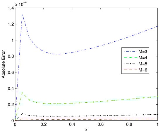
Figure 1. The absolute errors of Example 1 for quasilinearized semi-orthogonal B-spline wavelet method (QSOBWM) with $M=3,4,5,6$.

In order to compare with the second-kind Chebyshev polynomials method (SKCPM) in [8] and the fractional order Euler functions method (FEFsM) in [9], we computed the $L_2$ errors of the present scheme with various values of M and list the results in Table 2, where N denotes the maximal degree of the polynomials in the space spanned by all polynomials for SKCPM and FEFsM, and M indicates the truncation in the present scheme. The degree of all polynomials was no more than three when $m=4$ in the present scheme. Table 2 shows that the $L_2$ errors of the present scheme with $m=4$ were smaller.

Example 2.

Consider the following fractional Langevin equation [14]:

$$D^{{\alpha }_1}u\left(x\right)+D^{{\alpha }_2}u\left(x\right)+I^{\beta }u\left(x\right)=f\left(x\right),0<x<1,$$

(53)

with the initial condition

$$u\left(0\right)=0,$$

here $f\left(x\right)=\left(\frac{2.0x^{2-{\alpha }_1}}{\mathsf{\Gamma }\left(3.0-{\alpha }_1\right)}-\frac{x^{1-{\alpha }_1}}{\mathsf{\Gamma }\left(2.0-{\alpha }_1\right)}\right)+\left(\frac{2.0x^{2-{\alpha }_2}}{\mathsf{\Gamma }\left(3.0-{\alpha }_2\right)}-\frac{x^{1-{\alpha }_2}}{\mathsf{\Gamma }\left(2.0-{\alpha }_2\right)}\right)+\left(\frac{2.0x^{2+\beta }}{\mathsf{\Gamma }\left(3.0+\beta \right)}-\frac{x^{1+\beta }}{\mathsf{\Gamma }\left(2.0+\beta \right)}\right)$ and ${\alpha }_1,{\alpha }_2,\beta \in (0,1)$. The exact solution is given by $u\left(x\right)=x^2-x$.

Table 2. $L_2$ errors of QSOBWM, second-kind Chebyshev polynomials method (SKCPM) (in [8]), and FEFM (in [9]) for Example 1.

N	SKCPM	FEFsM $(\alpha =1)$	FEFsM $(\alpha =1.5)$	M	QSOBWM
2	$1.3426\times {10}^{-2}$	$1.0502\times {10}^{-2}$	$1.7511\times {10}^{-4}$	3	$9.6130\times {10}^{-5}$
4	$5.1379\times {10}^{-4}$	$2.6252\times {10}^{-4}$	$2.4436\times {10}^{-4}$	4	$2.5255\times {10}^{-5}$
6	$1.5578\times {10}^{-4}$	$6.6216\times {10}^{-5}$	$3.0232\times {10}^{-5}$	5	$6.5901\times {10}^{-6}$
8	$6.4612\times {10}^{-5}$	$4.8349\times {10}^{-4}$	$9.4123\times {10}^{-5}$	6	$1.7168\times {10}^{-6}$

We solved this problem by using the QSOBWM with $m=4$ and $M=3$ for fixed step size $h=\frac{1}{20}$. Table 3 exhibits the absolute errors, which demonstrates that the absolute errors of various values of ${\alpha }_1$, ${\alpha }_2$, and $\beta$ were less than ${10}^{-13}$, and that the computation took only 4.10 s. Furthermore, the results confirmed the effectiveness of this method. Figure 2 and Figure 3 depict the absolute errors of the present scheme for different ${\alpha }_1$ and $\beta$, respectively. Figure 2 presents the absolute errors of the present scheme with ${\alpha }_2=0.8$ and $\beta =0.3$ for various values of ${\alpha }_1$, while Figure 3 displays the absolute errors of the present scheme with ${\alpha }_1=0.5$ and ${\alpha }_2=0.8$ for several values of $\beta$. These graphs demonstrate that the approximate solutions agreed closely with the analytical result for various values of ${\alpha }_1$ and $\beta$, with absolute errors less than ${10}^{-13}$.

Table 3. Absolute errors of QSOBWM when $h=\frac{1}{20}$ for Example 2.

x	${\alpha }_1=0.99,{\alpha }_2=0.6,\beta =0.5$	${\alpha }_1=0.5,{\alpha }_2=0.8,\beta =0.3$	${\alpha }_1=0.1,{\alpha }_2=0.4,\beta =0.99$
0.1	$1.9582\times {10}^{-14}$	$2.0539\times {10}^{-15}$	$4.1633\times {10}^{-17}$
0.2	$1.6986\times {10}^{-14}$	$1.5266\times {10}^{-15}$	$2.7756\times {10}^{-17}$
0.3	$1.4932\times {10}^{-14}$	$1.1657\times {10}^{-15}$	$1.1102\times {10}^{-16}$
0.4	$1.3323\times {10}^{-14}$	$9.7145\times {10}^{-16}$	$1.6653\times {10}^{-16}$
0.5	$1.2046\times {10}^{-14}$	$8.8818\times {10}^{-16}$	$2.7756\times {10}^{-17}$
0.6	$1.0880\times {10}^{-14}$	$7.2164\times {10}^{-16}$	$5.5511\times {10}^{-17}$
0.7	$9.7700\times {10}^{-15}$	$5.2736\times {10}^{-16}$	$2.7756\times {10}^{-17}$
0.8	$8.6042\times {10}^{-15}$	$3.6082\times {10}^{-16}$	$8.3267\times {10}^{-17}$
0.9	$7.6328\times {10}^{-15}$	$2.9143\times {10}^{-16}$	$9.7145\times {10}^{-17}$

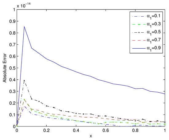
Figure 2. Absolute errors of Example 2 for QSOBWM with ${\alpha }_1=0.1,0.3,0.5,0.7,0.9$.

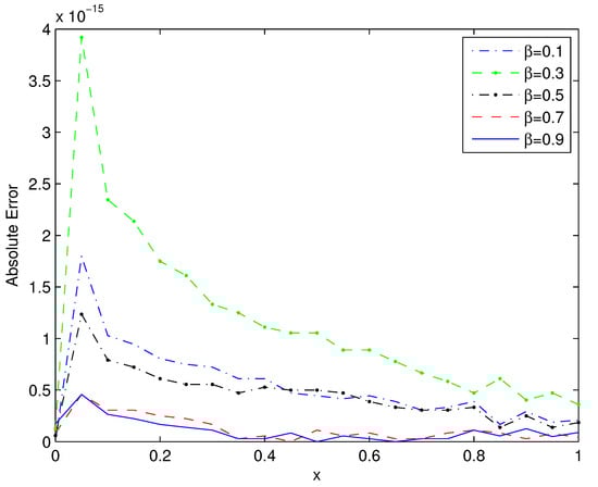
Figure 3. Absolute errors of Example 2 for QSOBWM with $\beta =0.1,0.3,0.5,0.7,0.9$.

In order to verify the performance of QSOBWM, as shown in Table 4, we calculated the $L_2$ error and $L_{\infty }$ error of the present scheme and the method in [14] for ${\alpha }_1=0.5,{\alpha }_2=0.8$, and $\beta =0.3$ with different grid sizes. The results demonstrated that the approximate results for the present scheme were closer to the analytical solutions than the method in [14].

Table 4. Comparison of the errors of QSOBWM and the method in [14] for Example 2.

Errors	Method of [14]			QSOBWM
	$\mathit{h}=\frac{1}{40}$	$\mathit{h}=\frac{1}{80}$	$\mathit{h}=\frac{1}{160}$	$\mathit{h}=\frac{1}{20}$	$\mathit{h}=\frac{1}{40}$
$\parallel u-\tilde{u}{\parallel }_{L_2}$	$2.3198\times {10}^{-3}$	$8.3037\times {10}^{-4}$	$9.9886\times {10}^{-6}$	$1.2270\times {10}^{-15}$	$5.7478\times {10}^{-16}$
$\parallel u-\tilde{u}{\parallel }_{L_{\infty }}$	$7.2983\times {10}^{-3}$	$2.7903\times {10}^{-3}$	$2.3399\times {10}^{-5}$	$3.4556\times {10}^{-15}$	$1.1102\times {10}^{-17}$

Some interesting phenomena are shown in Figure 1, Figure 2 and Figure 3. There may be two reasons: First, when $x=0$, the error is much closer to zero as the value at $x=0$ satisfies both the original equation and the initial value; however, the values with $x\in (0,1]$ only satisfy the original equation, which is more likely to have bigger errors. Second, it might be related to the reduced algebraic equations, which needs more exploration.

Example 3.

Consider the following fractional Duffing–Holmes model for a non-linear oscillator [31]:

$$D^{2}u\left(x\right)+0.5D^{\mu }u\left(x\right)-u\left(x\right)+u^3\left(x\right)=g\left(x\right),0<x<1$$

(54)

with the initial value:

$$u\left(0\right)=u^{\prime }\left(0\right)=0.$$

From [31], $u\left(x\right)=x^{\mu +2}sinx$ is the given exact solution.

We approximated the solution using QSOBWM with $m=4$ and different M ($M=3,4,5,6$). This problem was also solved by the spectral collocation method (SCM) in [31] with $\mu =0.5$ and $N=5,6,7,8,$ where N denotes the maximal degree of polynomials in the space formed by the basis of the method. In Table 5, we compare the $L_2$ errors and $L_{\infty }$ errors of the two methods mentioned above. The degree N of the polynomials in the present scheme was three. The $L_2$ and $L_{\infty }$ errors of the present scheme were much smaller than those of the SCM from Table 5. Moreover, the $L_2$ errors and $L_{\infty }$ errors of the present scheme decreased when M increased. Thus, the results were in accordance with the convergence analysis discussed in the previous section.

Table 5. Example 3: $L_2$ errors and $L_{\infty }$ errors with $\mu =0.5$ for spectral collocation method (SCM) and QSOBWM.

Methods	$\parallel \mathit{u}-\tilde{\mathit{u}}{\parallel }_{{\mathit{L}}_2}$	$\parallel \mathit{u}-\tilde{\mathit{u}}{\parallel }_{{\mathit{L}}_{\mathit{\infty }}}$
SCM
$N=5$	$8.237\times {10}^{-5}$	$2.204\times {10}^{-5}$
$N=6$	$2.291\times {10}^{-5}$	$8.859\times {10}^{-6}$
$N=7$	$1.467\times {10}^{-5}$	$4.763\times {10}^{-6}$
$N=8$	$6.885\times {10}^{-6}$	$2.714\times {10}^{-6}$
QSOBWM
$M=3$	$1.310\times {10}^{-5}$	$5.950\times {10}^{-5}$
$M=4$	$1.284\times {10}^{-6}$	$5.115\times {10}^{-7}$
$M=5$	$1.119\times {10}^{-7}$	$4.511\times {10}^{-8}$
$M=6$	$1.077\times {10}^{-8}$	$4.026\times {10}^{-9}$

Figure 4 depicts the analytical and numerical results of the present scheme with $M=3$ for $\mu =0.01,0.3,0.5,0.7,$ and $0.99$. The figure demonstrates that the numerical results tended to the analytical solution for different values of $\mu$.

Example 4.

Consider the following multi-term fractional non-linear boundary value problem [11,12]:

$$D^{2}u\left(x\right)+\mathsf{\Gamma }\left(\frac{4}{5}\right)\sqrt[5]{x^6}{D}^{\frac{6}{5}}u\left(x\right)+\frac{11}{9}\mathsf{\Gamma }\left(\frac{6}{5}\right)\sqrt[6]{x}{D}^{\frac{1}{6}}u\left(x\right)-{\left(Du\left(x\right)\right)}^2=2+\frac{1}{10}{x}^2,$$

(55)

with boundary conditions:

$$u\left(0\right)=1,u\left(1\right)=2.$$

The exact solution of this problem is $u\left(x\right)=x^2+1$.

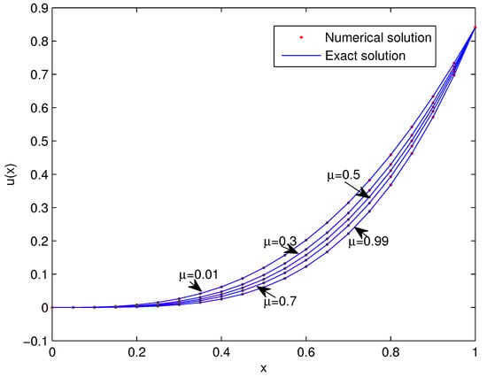
Figure 4. Analytical and approximate results of QSOBWM for $M=3$ with $\mu =0.01,0.3,0.5,0.7,$ and $0.99$ for Example 3.

The problem was resolved by the B-spline operational matrix method (BSOMM) [12] and the Bernstein operational matrix method (BOMM) [11], respectively. We also solved the example by applying the present scheme with $m=4$ and list the values of the $L_2$ and $L_{\infty }$ errors of the three methods in Table 6. The $L_2$ errors of the present scheme achieved ${10}^{-14}$ within 7.98 s. As shown in Table 6, the present scheme was the most accurate.

Table 6. The $L_2$ errors and $L_{\infty }$ errors of QSOBWM, B-spline operational matrix method (BSOMM) (in [12]), and Bernstein operational matrix method (BOMM) (in [11]) for Example 4.

$\mathit{Errors}$	BSOMM		BOMM		QSOBWM
	$\mathit{M}=\mathbf{5}$	$\mathit{M}=\mathbf{7}$	$\mathit{N}=\mathbf{16}$	$\mathit{N}=\mathbf{20}$	$\mathit{M}=\mathbf{3}$	$\mathit{M}=\mathbf{4}$
$\parallel u-\tilde{u}{\parallel }_{L_2}$	$1.2\times {10}^{-4}$	$7.6\times {10}^{-6}$	$2.3\times {10}^{-8}$	$7.9\times {10}^{-9}$	$7.315\times {10}^{-14}$	$1.335\times {10}^{-14}$
$\parallel u-\tilde{u}{\parallel }_{L_{\infty }}$	$3.3\times {10}^{-4}$	$2.1\times {10}^{-5}$	$5.5\times {10}^{-8}$	$1.9\times {10}^{-8}$	$1.112\times {10}^{-13}$	$2.043\times {10}^{-14}$

7. Conclusions

In this article, the quasilinearized semi-orthogonal B-spline wavelet method is proposed to approximate multi-term non-linear fractional order equations containing fractional integrals and derivatives. The proposed scheme significantly reduces the computational complexity of solving non-linear fractional order equations by using the semi-orthogonal B-spline wavelet collocation method. The solution procedure for approximating non-linear fractional equations is described. we also discuss the convergence properties of the present scheme. As the initial and boundary conditions are both considered during the process of function approximation, this method can be applied to solving both initial and boundary value problems of fractional order. Illustrative examples and comparison results were given to demonstrate the efficiency and accuracy of the proposed scheme.

References

- Bagley, R.L.; Torvik, P.J. A theoretical basis for the application of fractional calculus to viscoelasticity. J. Rheol. 1983, 27, 201–210. [Google Scholar] [CrossRef]
- El-Sayed, A.M.A.; Gaafar, F.M. Fractional calculus and some intermediate physical processes. Appl. Math. Comput. 2003, 144, 117–126. [Google Scholar] [CrossRef]
- Elwakil, A.S. Fractional-order circuits and systems: An emerging interdisciplinary research area. IEEE Circ. Syst. Mag. 2010, 10, 40–50. [Google Scholar] [CrossRef]
- Miljkovic, N.; Popovic, N.; Djordjevic, O.; Konstantinovic, L.; Sekara, T.B. ECG artifact cancellation in surface EMG signals by fractional order calculus application. Comput. Methods Programs Biomed. 2017, 140, 259–264. [Google Scholar] [CrossRef] [PubMed]
- Lai, Q.H.; Diao, Z.J.; Kong, L.L.; Adidharma, H.; Fan, M.H. Amine-impregnated silicic acid composite as an efficient adsorbent for CO2 capture. Appl. Energy 2018, 223, 293–301. [Google Scholar] [CrossRef]
- Machado, J.T.; Kiryakova, V.; Mainardi, F. Recent history of fractional calculus. Commun. Nonlinear Sci. 2011, 16, 1140–1153. [Google Scholar] [CrossRef]
- Doha, E.H.; Bhrawy, A.H.; Ezz-Eldien, S.S. A Chebyshev spectral method based on operational matrix for initial and boundary value problems of fractional order. Comput. Math. Appl. 2011, 62, 2364–2373. [Google Scholar] [CrossRef]
- Nemati, S.; Sedaghat, S.; Mohammadi, I. A fast numerical algorithm based on the second kind Chebyshev polynomials for fractional integro-differential equations with weakly singular kernels. J. Comput. Appl. Math. 2016, 308, 231–242. [Google Scholar] [CrossRef]
- Wang, Y.X.; Zhu, L.; Wang, Z. Fractional-order Euler functions for solving fractional integro-differential equations with weakly singular kernel. Adv. Differ. Equ. 2018, 2018, 254. [Google Scholar] [CrossRef]
- Zeid, S.S. Approximation methods for solving fractional equations. Chaos Solitons Fract. 2019, 125, 171–193. [Google Scholar] [CrossRef]
- Saadatmandi, A. Bernstein operational matrix of fractional derivatives and its applications. Appl. Math. Model. 2014, 38, 1365–1372. [Google Scholar] [CrossRef]
- Lakestani, M.; Dehghan, M.; Irandoust-Pakchin, S. The construction of operational matrix of fractional derivatives using B-spline functions. Commun. Nonlinear Sci. 2012, 17, 1149–1162. [Google Scholar] [CrossRef]
- Kojabad, E.A.; Rezapour, S. Approximate solutions of a sum-type fractional integro-differential equation by using Chebyshev and Legendre polynomials. Adv. Differ. Equ. 2017, 2017, 351. [Google Scholar]
- Zheng, Y.Y.; Zhao, Z.G.; Cui, Y.F. The discontinuous Galerkin finite element approximation of the multi-order fractional initial problems. Appl. Math. Comput. 2019, 348, 257–269. [Google Scholar] [CrossRef]
- Shiralashetti, S.C.; Deshi, A.B. An efficient Haar wavelet collocation method for the numerical solution of multi-term fractional differential equations. Nonlinear Dynam. 2016, 83, 293–303. [Google Scholar] [CrossRef]
- Rahimkhani, P.; Ordokhani, Y.; Lima, P.M. An improved composite collocation method for distributed-order fractional differential equations based on fractional Chelyshkov wavelets. Appl. Numer. Math. 2019, 145, 1–27. [Google Scholar] [CrossRef]
- Nevels, R.D.; Goswami, J.C. Semi-orthogonal versus orthogonal wavelet basis sets for solving integral equations. IEEE Trans. Antenn. Propag. 1997, 45, 1332–1339. [Google Scholar] [CrossRef]
- Maleknejad, K.; Nouri, K.; Sahlan, M.N. Convergence of approximate solution of nonlinear Fredholm-Hammerstein integral equations. Commun. Nonlinear Sci. 2010, 15, 1432–1443. [Google Scholar] [CrossRef]
- Aram, P.; Freestone, D.R.; Dewar, M.; Scerri, K.; Jirsa, V.; Grayden, D.B.; Kadirkamanathan, V. Spatiotemporal multi-resolution approximation of the Amari type neural field model. Neuroimage 2013, 66, 88–102. [Google Scholar] [CrossRef]
- Liu, C.; Zhang, X.M.; Wu, B.Y. Numerical solution of fractional differential equations by semiorthogonal B-spline wavelets. In Mathematical Methods in the Applied Sciences; Wiley Online Library: Hoboken, NJ, USA, 2019; pp. 1–14. [Google Scholar]
- Saeed, U.; Rehman, M.U. Haar wavelet-quasilinearization technique for fractional nonlinear differential equations. Appl. Math. Comput. 2013, 220, 630–648. [Google Scholar] [CrossRef]
- Liu, Z.H.; Wang, R. Quasilinearization method for fractional differential equations with delayed arguments. Appl. Math. Comput. 2014, 248, 301–308. [Google Scholar] [CrossRef]
- Hosseinnia, S.H.; Ranjbar, A.; Momani, S. Using an enhanced homotopy perturbation method in fractional differential equations via deforming the linear part. Comput. Math. Appl. 2008, 56, 3138–3149. [Google Scholar] [CrossRef]
- Baleanu, D.; Agheli, B.; Darzi, R. An optimal method for approximating the delay differential equations of noninteger order. Adv. Differ. Equ. 2018, 2018, 284. [Google Scholar] [CrossRef]
- Samko, S.G.; Kilbas, A.A.; Marichev, O.I. Fractional Integrals and Derivatives: Theory and Applications; Gordon and Breach Science Publishers: New York, NY, USA, 1993. [Google Scholar]
- Podlubny, I. Fractional Differential Equations; Academic Press: New York, NY, USA, 1999. [Google Scholar]
- Chui, C.K.; Quak, E. Wavelets on a bounded interval. In Numerical Methods in Approximation Theory; Braess, D., Schumaker, L.L., Eds.; Birkhäuser-Verlag, Basel: College Station, TX, USA, 1992; pp. 53–75. [Google Scholar]
- Li, X.X. Numerical solution of fractional differential equations using cubic B-spline wavelet collocation method. Commun. Nonlinear Sci. 2012, 17, 3934–3946. [Google Scholar] [CrossRef]
- Mandelzweig, V.B.; Tabakin, F. Quasilinearization approach to nonlinear problems in physics with application to nonlinear ODEs. Comput. Phys. Commun. 2001, 141, 268–281. [Google Scholar] [CrossRef]
- Volterra, V. Theory of Functionals and of Integral and Integro-Differential Equations; Dover: New York, NY, USA, 2005. [Google Scholar]
- Zaky, M.A.; Ameen, I.G. On the rate of convergence of spectral collocation methods for nonlinear multi-order fractional initial value problems. Comput. Appl. Math. 2019, 38, 144. [Google Scholar] [CrossRef]
© 2020 by the authors. Licensee MDPI, Basel, Switzerland. This article is an open access article distributed under the terms and conditions of the Creative Commons Attribution (CC BY) license (http://creativecommons.org/licenses/by/4.0/).