Abstract
We consider the problem of pricing American options using the generalized Black–Scholes model. The generalized Black–Scholes model is a modified form of the standard Black–Scholes model with the effect of interest and consumption rates. In general, because the American option problem does not have an exact closed-form solution, some type of approximation is required. A simple numerical method for pricing American put options under the generalized Black–Scholes model is presented. The proposed method corresponds to a free boundary (also called an optimal exercise boundary) problem for a partial differential equation. We use a transformed function that has Lipschitz character near the optimal exercise boundary to determine the optimal exercise boundary. Numerical results indicating the performance of the proposed method are examined. Several numerical results are also presented that illustrate a comparison between our proposed method and others.
Keywords:
American option pricing; generalized Black–Scholes partial differential equation; optimal exercise boundary; transformed function JEL Classification:
C60; G13
1. Introduction
Hedging and pricing are important issues in derivative securities. European and American options can be exercised only on the expiration date and at any time until the expiration date, respectively. For European options, closed-form solutions are derived from Black and Scholes [1]’s and Merton [2]’s celebrated papers. However, no analogous results exist for American options, because the early exercise possibility of American options leads to complications in analytical calculations. The option holder’s purchase of this early exercise right changes the problem into the so-called free boundary value problem. McKean [3] and Van Moerbeke [4] proved that the valuation of American options constitutes a free boundary problem and they studied the properties of the free boundary (generally it is called an optimal exercise boundary). Therefore, financial researchers have paid attention to developing approximation methods to price American options. For example, hybrid methods combine analytical and numerical approximations. Kim et al. [5] used numerical methods, and Bouchard et al. [6] used Monte Carlo simulations. More specifically, Chockalingam and Muthuraman [7] adopted an approximate moving boundary method. Additionally, to fix the boundary and solve the resulting nonlinear problem, front-fixing methods developed by Wu and Kwok [8] and Nielsen et al. [9] apply a nonlinear transformation.
However, unlike previous studies, Alghalith [10] recently introduced a closed formula for pricing American options and an exact upper bound for the price. This formula is the first to explicitly and directly link the difference between the prices of an American option and its European counterpart to the interest rate.
In this paper, the assumptions of the Black–Scholes [1] and Alghalith [10] models are adopted to develop a numerical method that uses the transformed function to value American put options. The Alghalith [10] model is called the generalized Black–Scholes model, which is a modified form of the standard Black–Scholes model, including the effect of interest and consumption rates. The main contribution of this paper is the development of a numerical method for finding the optimal exercise boundary of American put options under the generalized Black–Scholes model. Since the buyer of an option has the right to exercise it, and since when exercising the option, the buyer will choose an optimal exercise strategy to maximize profits, the writer of the option will suffer same amount of loss. In fact, the value of the option to the option writer comes from the compensation they receive. In this paper, utilizing the optimal exercise strategy means finding the optimal exercise boundary exactly. Therefore, the proposed method is of great significance. The proposed method is mathematically proven by determining this boundary using a transformed function. We exploit a transformed function that has the Lipschitz character to prevent the solution surface from degenerating near the optimal exercise boundary. By constructing a relation between the transformed function and the optimal exercise boundary, and using the properties of the transformed function, the optimal exercise boundary can be easily determined. After determining the optimal exercise boundary, we calculate the value of the American put options by applying finite difference method (FDM) and use the Crank–Nicolson method in time discretization. Typically, the optimal exercise boundary may not be located at grid points. Therefore, the interpolation method is used to determine the value of the American put option under the generalized Black–Scholes model. For calculating the optimal exercise boundary and pricing American put options, fast and accurate results are provide through our method. Additionally, several numerical results are presented to illustrate comparisons between the proposed method and others. Finally, the result of our method is compared with that of the closed formula of Alghalith [10] for pricing the American options.
This paper is further organized in the following manner. In Section 2, the generalized Black–Scholes model and the free boundary value problem for American put options have been introduced. Section 3 discusses the use of the transformed function to calculate the optimal exercise boundary as reasonable and presents the numerical method to value American put options under the generalized Black–Scholes model. Numerical examples, results, and a comparison with other models are presented in Section 4. Finally, Section 5 provides a summary of the paper.
2. Preliminaries
This section presents a mathematical problem for pricing an American put option under the generalized Black–Scholes model. The assumption of the models of Black–Scholes [1] and Alghalith [10] are adopted. Let denote the value of an underlying asset price as a function of the current time t. is assumed to follow the process:
where and are the constant interest rate and the volatility, respectively, and is a standard Brownian motion. Well-known in the literature is that the wealth process satisfies this equation (see [11]):
where is the risky portfolio process and is the consumption rate (defined as the amount of money consumed at time t). Consumption is possible by the option writer if the buyer/holder did not exercise at the optimal exercise time because, in this case, the writer gains extra money (in excess of the hedging need) that can be consumed and , where is the price of the American put option.
Therefore, given the assumptions of the Black–Scholes [1] model and following Alghalith [10], the modified Black–Scholes partial differential equation(PDE) is
where and refer to partial derivatives. Following the literature (see [11]), c in the previous PDE is replaced by its average ; this expression is substituted into (3) to obtain
where (see [10]).
The payoffs for an American put option at the underlying asset price with exercise price K and time T to expiration are
The valuation of an American put option is denoted as , and is the time to expiration for . As is well-known [12], a function exists that is commonly referred to as the optimal exercise boundary, such that the option is exercised for and
In this case, the region in which it is optimal to exercise, generally called the “exercise region” is defined as . Instead, for , the American option price satisfies the following generalized Black–Scholes equation:
where . In this case, the region in which it is optimal to hold, generally called the “continuation region” is defined as . Further, we assume that the optimal exercise boundary decreases continuously with .
Mckean’s analysis [3] implies that the value of an American put option and the exercise boundary jointly solve the free boundary problem consisting of (7) subject to the following boundary conditions:
and the initial condition
For more detailed information on Equations (7)–(11), please see Reference [13].
To find the optimal exercise boundary, we review a transformed function developed by Kim et al. [14] as follows:
This transformed function ensures that the solution surface in the exercise (continuation) region is a horizontal (inclined) plane. The transformed function forms a sufficiently large angle for which the horizontal line corresponds to the exercise region, rendering the borderline easily distinguishable (see Figure 1). The function also has a Lipschitz character with non-singularity and non-degeneracy near the optimal exercise boundary (i.e., the optimal exercise boundary is easily identified).
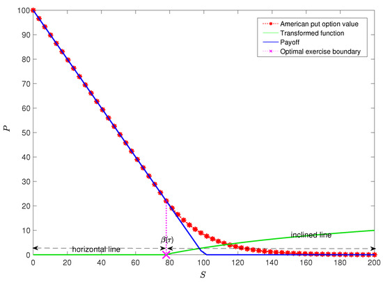
Figure 1.
Transformed function.
3. Numerical Method under the Generalized Black–Scholes Model
The transformed function from the PDE is derived to determine the optimal exercise boundary from the Taylor series. Following Theorem 1, an angle between the exercise region and the Q line is obtained such that for some constants and .
Theorem 1.
Let
Here, Q has a Lipschitz character with non-singularity and non-degeneracy near the optimal exercise boundary. Then,
where
Proof of Theorem 1.
From , the following relations near the optimal exercise boundary are obtained:
Plugging Equation (13) into Equation (7) leads to Q, which satisfies the following equation:
The following is obtained:
near the optimal exercise boundary(: as ). More precisely, we have
which leads to
For every , because , is obtained. Additionally,
and
Therefore,
Then, , where
and
□
For , Equation (7) becomes the standard Black–Scholes equation. This theorem derived the result for in Equation (7).
For discretization , a two-dimensional mesh in the first quadrant of the plane is introduced. This problem is solved by applying the FDM and dividing the time interval into N subintervals and the stock price interval into M subintervals A numerical scheme that allows for the grid values to be computed is defined. For this problem, is given, and the goal is to compute .
To find , the relationship between Q and is defined. To obtain , should be known. The optimal exercise boundary does not depend on a grid point because it is usually placed between grids. This means an FDM with a nonuniform mesh must be used. Therefore, and then is found. The generalized Black–Scholes Equation (7) may be approximated as the following difference equation:
The central difference is used for derivatives, and a cubic spline interpolation is applied to find and . Finally, the following is obtained:
Theorem 2.
We suppose thatis known, thensatisfies
where
where
Proof of Theorem 2.
Because , we have a second order Taylor expansion of Q:
To find , the partial derivative is calculated with respect to S in (7) to obtain
Given from Equation (13), is calculated. From Equation (10), this gives , where is the rate of change of with respect to time, which results in the following equation near the optimal exercise boundary ():
4. Numerical Results
This section provides numerical examples to illustrate the use of the proposed method to value American put options under the generalized Black–Scholes model. The numerical simulations are performed on a personal computer with an Intel Core i5 2.30 GHz and 8.00 GB RAM, and the software programs are written in MATLAB(R2019a). A FDM with Crank–Nicolson scheme is used for the proposed method.
Figure 2 plots the optimal exercise boundaries of American put options under the generalized Black–Scholes model with specified parameters. Option investors should have a significant interest in understanding the optimal exercise boundary of American options. A computational domain with 200 spatial steps and 1000 time steps is constructed. All else being fixed, Figure 2 indicates that the optimal exercise boundary of a put option shifts downward as r(and ) decreases. When the interest rate increases, exercising the option early for cash is more attractive because of a higher return from interest rates.
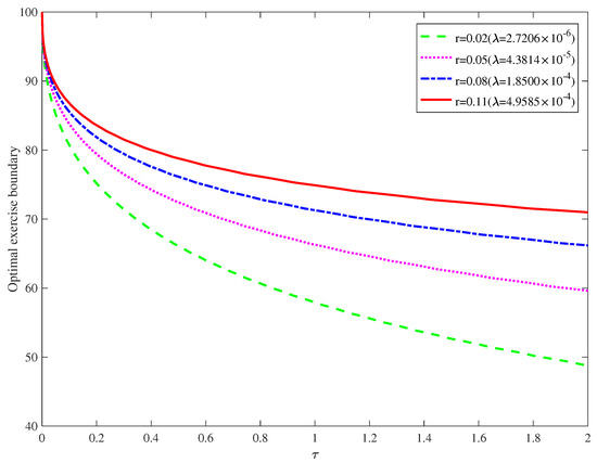
Figure 2.
Optimal exercise boundary for different r(and ). ().
Figure 3 illustrates the optimal exercise boundary for the expected consumption value and r with the parameter set and . For a specific variable, , that is, the optimal exercise boundary in the standard Black–Scholes model is compared with the optimal exercise boundary in the generalized model. The same parameters are used, which show that the optimal exercise boundary value is larger for the standard Black–Scholes model than the generalized Black–Scholes model.
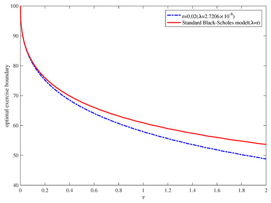
Figure 3.
Optimal exercise boundary for (and also ). ().
Figure 4 demonstrates the American put option values of , and 0.11 (, , , and ). Table 1 presents the American put option values obtained for specific parameters. Note that the discrete meshes of nodes is plotted in Figure 4 and Table 1. A higher expected consumption value of results in lower values of the American put option. As interest rates in the economy increase, the expected growth rate of a stock price tends to increase, whereas the present value of any future cash flows received by an option holder decreases. Both of these effects tend to decrease the value of a put option. Hence, put option prices decline as the risk-free interest rate increases.
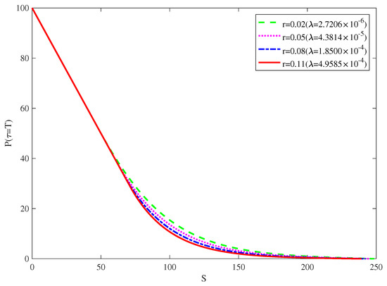
Figure 4.
American put option values for different values of r(and ). ().

Table 1.
American put option values.
Table 2 provides a comparison of American put option values calculated using various methods with . Benchmark results are obtained using the Binomial method with 10,000 time steps. In Table 2, the root mean squared error (RMSE) is calculated for using the proposed method. By doing so, the numerical convergence of the method is illustrated. The parameter values used to calculate the American put option values are , and , and discrete meshes of 125 × 25, 250 × 50, 500 × 100, 1000 × 200, 2000 × 400 and 4000 × 800 are checked. Computation errors are deduced to compare with the results [15] obtained through other numerical methods, including the front-fixing method (front-fixing) developed by Wu and Kwok [8], the finite difference implementation of the moving boundary method (MBM-FDM) developed by Muthuraman [16], and the simple numerical method (simple method) developed by B.J. Kim, Y.-K. Ma, and H.J. Choe [15]. Benchmark results are obtained using binomial method (binomial) developed by Cox et al. [17], and we consider these results to be the exact American put option values.
Table 2.
Comparison of value of American put options calculated by various methods.
The five different methods have similar American put option values. While the proposed method may not be the best options trading method, determining the optimal exercise boundary is an important problem associated with American options. The proposed method can be easily applied because only the equation has to be solved to determine the optimal exercise boundary. Therefore, the proposed method can be used to accurately calculate the optimal exercise boundary.
Finally, Table 3 presents the reference [10] value(closed-form formula) compared with the value of this paper’s model when and , and when and 2. We use the parameter values and to calculate the American put option value. In any case, the result of the proposed method can obtain a value close to that of reference [10] in a mesh. In addition, when the maturity is short, a result close to [10] is obtained. The larger the mesh size, the larger the difference between the proposed method and the result of [10]. Therefore, [10] can be used to approximate the value of an option when its maturity is short, and is calculated by a formula. However, for American options, determining the optimal exercise boundary is the most important issue. The proposed method can be used in any situation, including short or long maturity.
Table 3.
Comparison of value of American put options with closed-form formula.
5. Final Remarks
In this paper, a simple numerical method is presented to find the optimal exercise boundary in an American put option under the generalized Black–Scholes model. Most importantly, a Lipschitz curve is found that avoids the degeneracy and singularity of the solution line near the optimal exercise boundary because the solution line near the optimal exercise boundary needs to be carefully examined. Of course, the American option value can be easily calculated, as suggested by [10]. However, because the American option is a sensitive free boundary problem, pinpointing the free boundary is more important. It is employed to easily determine the optimal exercise boundary by solving a quintic equation in a time-recursive manner. The generalized Black–Scholes model is a modified form of the standard Black–Scholes model with the effect of interest and consumption rates. We present this effect and show several numerical results that illustrate a comparison to other methods. Therefore, in such a rapidly changing environment, the straightforward method of this paper is a very powerful tool for understanding financial markets.
Funding
The author is supported by the National Research Foundation of Korea (NRF) under Grant No. 2019R1G1A1099148.
Conflicts of Interest
The author declares no conflict of interest.
References
- Black, F.; Scholes, M. The pricing of Options and Corporate Liabilities. J. Political Econ. 1973, 81, 637–659. [Google Scholar] [CrossRef]
- Merton, R.C. Theory of rational option pricing. Bell J. Econ. Manag. Sci. 1973, 4, 141–183. [Google Scholar] [CrossRef]
- McKean, H.P., Jr. Appendix: A free boundary problem for the heat equation arising from a problem in mathematical economics. Ind. Manag. Rev. 1965, 6, 32–39. [Google Scholar]
- Van Moerbeke, P. On optimal stopping and free boundary problems. Arch. Ration. Mech. Anal. 1976, 60, 101–148. [Google Scholar] [CrossRef]
- Kim, I.J.; Jang, B.G.; Kim, K.T. A simple iterative method for the valuation of American options. Quant. Financ. 2013, 13, 885–895. [Google Scholar] [CrossRef]
- Bouchard, B.; Chau, K.W.; Manai, A.; Sid-Ali, A. Monte-Carlo methods for the pricing of American options: A semilinear BSDE point of view. ESAIM Proc. Surv. 2019, 65, 294–308x. [Google Scholar] [CrossRef]
- Chockalingam, A.; Muthuraman, K. An approximate moving boundary method for American option pricing. Eur. J. Oper. Res. 2015, 240, 431–438. [Google Scholar] [CrossRef]
- Wu, L.; Kwok, Y.K. A front-fixing finite difference method for the valuation of American options. J. Financ. Eng. 1997, 6, 83–97. [Google Scholar]
- Nielsen, B.F.; Skavhaug, O.; Tveito, A. Penalty and frontfixing methods for the numerical solution of American option problems. J. Comput. Financ. 2002, 5, 69–97. [Google Scholar] [CrossRef]
- Alghalith, M. Pricing the American options: A closed-form, simple formula. Phys. A Stat. Mech. Appl. 2019, 548, 123873. [Google Scholar] [CrossRef]
- Cvitanić, J.; Zapatero, F. Introduction to the Economics and Mathematics of Financial Markets; MIT Press: Cambridge, MA, USA, 2004. [Google Scholar]
- Wilmott, P.; Howison, S.; Dewynne, J. The Mathematics of Financial Derivatives; Cambridge University Press: Cambridge, UK, 1995. [Google Scholar]
- Carr, P.; Jarrow, R.; Myneni, R. Alternative characterizations of American put options. Math. Financ. 1992, 2, 87–106. [Google Scholar] [CrossRef]
- Kim, B.J.; Ahn, C.; Choe, H.J. Direct computation for American put option and free boundary using finite difference method. Jpn. J. Ind. Appl. Math. 2013, 30, 21–37. [Google Scholar] [CrossRef]
- Kim, B.J.; Ma, Y.K.; Choe, H.J. A Simple method for pricing an American put option. J. Appl. Math. 2013, 2013, 128025. [Google Scholar] [CrossRef]
- Muthuraman, K. A moving boundary approach to American option pricing. J. Econ. Dyn. Control 2008, 32, 3520–3537. [Google Scholar] [CrossRef]
- Cox, J.C.; Ross, S.A.; Rubinstein, M. Option pricing: A simplified approach. J. Financ. Econ. 1979, 7, 229–263. [Google Scholar] [CrossRef]


© 2020 by the author. Licensee MDPI, Basel, Switzerland. This article is an open access article distributed under the terms and conditions of the Creative Commons Attribution (CC BY) license (http://creativecommons.org/licenses/by/4.0/).