A Crank–Nicolson Finite Volume Element Method for Time Fractional Sobolev Equations on Triangular Grids

Abstract

In this paper, a finite volume element (FVE) method is proposed for the time fractional Sobolev equations with the Caputo time fractional derivative. Based on the $L1$-formula and the Crank–Nicolson scheme, a fully discrete Crank–Nicolson FVE scheme is established by using an interpolation operator $I_h^{*}$. The unconditional stability result and the optimal a priori error estimate in the $L^2(\Omega )$-norm for the Crank–Nicolson FVE scheme are obtained by using the direct recursive method. Finally, some numerical results are given to verify the time and space convergence accuracy, and to examine the feasibility and effectiveness for the proposed scheme.

1. Introduction

Fractional partial differential equations (FPDEs) have received extensive attentions by more and more scholars, and have been widely applied in many fields of science and engineering [1,2]. Many practical problems can be portrayed very well by the some FPDEs, such as fractional (reaction) diffusion equations [3,4,5,6,7,8,9,10,11,12], fractional Allen–Cahn equations [13,14,15], fractional Cable equations [16,17,18], and fractional mobile/immobile transport equations [19,20,21]. In the past few decades, a large number of numerical methods [22,23,24] have been proposed and used to solve the FPDEs, which have achieved excellent theoretical and numerical results. Recently, some scholars began to propose some numerical methods to solve fractional Sobolev equations. Liu et al. [25] constructed a modified reduced-order finite element scheme to solve the time fractional Sobolev equations by using the proper orthogonal decomposition technique [26,27], and obtained the stability and convergence results. Haq and Hussain [28] proposed a meshfree spectral method for the time fractional Sobolev equations by using radial basis functions and point interpolation method. Beshtokov [29] proposed a finite difference method to solve the time fractional Sobolev-type equations with memory effect.

In this paper, we study a Crank–Nicolson finite volume element method to solve the following time fractional Sobolev equations with the initial and boundary conditions

$$\begin{array}{c}\hfill \left\{\begin{array}{cc}{\displaystyle \frac{\partial u(\mathit{x},t)}{\partial t}}-{\kappa }_1{\displaystyle \frac{{\partial }^{\alpha }\Delta u(\mathit{x},t)}{\partial t^{\alpha }}}-{\kappa }_2\Delta u(\mathit{x},t)=f(\mathit{x},t),\hfill & (\mathit{x},t)\in \Omega \times J,\hfill \\ u(\mathit{x},t)=0,\hfill & (\mathit{x},t)\in \partial \Omega \times \overline{J},\hfill \\ u(\mathit{x},0)=u_0\left(\mathit{x}\right),\hfill & \mathit{x}\in \overline{\Omega },\hfill \end{array}\right.\end{array}$$

(1)

where $J=(0,T]$ with a positive constant T. Here, we assume that $\Omega \subset R^2$ is a bounded convex polygonal region with boundary $\partial \Omega$, the coefficients ${\kappa }_1$ and ${\kappa }_2$ are two positive constants. Moreover, we assume that the initial data $u_0\left(\mathit{x}\right)$ and source function $f(\mathit{x},t)$ are smooth enough. In (1), ${\partial }^{\alpha }/\partial t^{\alpha }$ is the Caputo time fractional derivative with order $\alpha$ $(0<\alpha <1)$ defined by

$$\begin{array}{c}\hfill {\displaystyle \frac{{\partial }^{\alpha }\varphi (\mathit{x},t)}{\partial t^{\alpha }}}={\displaystyle \frac{1}{\Gamma (1-\alpha )}}{\int }_0^t{\displaystyle \frac{\partial \varphi (\mathit{x},s)}{\partial s}}{\displaystyle \frac{ds}{{(t-s)}^{\alpha }}},\mathrm{for}\mathrm{a}\mathrm{given}\mathrm{function}\varphi (\mathit{x},t).\end{array}$$

(2)

In recent years, the finite volume element (FVE) methods [30,31,32,33,34] have been applied by more and more scholars to solve some FPDEs numerically. Sayevand and Arjang [35] proposed an FVE method for the sub-diffusion equation with the Caputo fractional derivative. Karaa et al. [36] adopted a piecewise linear discontinuous Galerkin method in time, and constructed an FVE scheme for the sub-diffusion equation with the Riemann-Liouville fractional derivative. Karaa and Pani [37] constructed two fully discrete FVE schemes to solve the time fractional sub-diffusion equation with smooth and nonsmooth initial datas, in which the Riemann–Liouville fractional derivative was approximated by using convolution quadrature generated by two different difference schemes. Badr et al. [38] proposed a B-spline FVE method for the time fractional advection-diffusion problem with the Caputo fractional derivative, and gave the stability analysis. Zhao et al. [39] designed an fully discrete FVE scheme to solve the nonlinear time fractional mobile/immobile transport equations based on the weighted and shifted Grünwald difference (WSGD) formula, and obtained the unconditional stability and optimal error estimates.

In this paper, the main aim was to establish a fully discrete FVE scheme to solve the time fractional Sobolev equation by using the Crank–Nicolson scheme. In spatial discretization, we use the classical FVE method, which can maintain the local conservation of some physical quantities, and this is very important in numerical computing. In temporal discretization, we apply the Crank–Nicolson scheme to discretize the equation at the time node $t_{n+1/2}$ on the whole, and combine the $L1$-formula [40,41] to discretize the Caputo time fractional derivative ${\partial }^{\alpha }\Delta u/\partial t^{\alpha }$, so that the time convergence accuracy is $O\left({\tau }^{2-\alpha }\right)$. In our theoretical analysis, we specially adopt the recursive analysis method, and obtain the unconditional stability result and the optimal a priori error estimate in the $L^2(\Omega )$-norm. Moreover, we provide some numerical results to verify the theoretical result, and to examine the feasibility and effectiveness of the fully discrete FVE scheme.

The remainder part of this paper is organized as follows. In Section 2, a Crank–Nicolson FVE scheme for the time fractional Sobolev Equation (1) is proposed. In Section 3, the unconditional stability analysis for the Crank–Nicolson FVE scheme is derived in detail. The a prioir error estimate is given in Section 4. Finally, in Section 5, some numerical results are given to illustrate the feasibility and effectiveness. Furthermore, throughout the article, we adopt the mark C to denote a generic positive constant, which is independent of the mesh parameters.

2. Crank–Nicolson Finite Volume Element Method

We first discretize the time (fractional) derivative. Let $0=t_0<t_1<\cdots <t_N=T$ be an equidistant grid for the time interval $[0,T]$ and $t_n=n\tau$, $n=0,1,\cdots ,N$, where the time step $\tau =T/N$ and N is a positive integer. For a given function $\phi$, we denote ${\phi }^n=\phi \left(t_n\right)$, ${\phi }^{n+\frac{1}{2}}=\frac{{\phi }^n+{\phi }^{n+1}}{2}$, and apply ${\tilde{\partial }}_t{\phi }^{n+\frac{1}{2}}=\frac{{\phi }^{n+1}-{\phi }^n}{\tau }$ to approximate $\frac{\partial \phi (\mathit{x},t)}{\partial t}$ at $t=t_{n+\frac{1}{2}}=\frac{t_{n+1}+t_n}{2}$, that is

$$\begin{array}{c}\hfill \frac{\partial \phi (\mathit{x},t)}{\partial t}{|}_{t_{n+\frac{1}{2}}}={\tilde{\partial }}_t{\phi }^{n+\frac{1}{2}}+E_{t,\phi }\left(t_{n+\frac{1}{2}}\right).\end{array}$$

(3)

where $E_{t,\phi }\left(t_{n+\frac{1}{2}}\right)$ is the truncation error.

For approximating the Caputo time fractional derivative $\frac{{\partial }^{\alpha }\phi (\mathit{x},t)}{\partial t^{\alpha }}$ at $t=t_{n+\frac{1}{2}}$, following References [40,41], we introduce the $L1$-formula as follows

$$\begin{array}{cc}\hfill {\displaystyle \frac{{\partial }^{\alpha }\phi (\mathit{x},t_n)}{\partial t^{\alpha }}}& =\frac{1}{\Gamma (1-\alpha )}{\int }_0^{t_n}\frac{\partial \phi (\mathit{x},s)}{\partial s}\frac{\mathrm{d}s}{{(t_n-s)}^{\alpha }}\hfill \\ \hfill & =\frac{{\tau }^{1-\alpha }}{\Gamma (2-\alpha )}\sum _{k=0}^{n-1}{b}_k\frac{\phi (\mathit{x},t_{n-k})-\phi (\mathit{x},t_{n-k-1})}{\tau }+R_t^n\left(\phi \right)\hfill \\ \hfill & =\frac{{\tau }^{1-\alpha }}{\Gamma (2-\alpha )}\sum _{k=0}^{n-1}{b}_k\frac{{\phi }^{n-k}-{\phi }^{n-k-1}}{\tau }+R_t^n\left(\phi \right)\hfill \end{array}$$

(4)

where $b_k={(k+1)}^{1-\alpha }-k^{1-\alpha }$, $R_t^n\left(\phi \right)$ is the truncation error. We denote

$$\begin{array}{c}\hfill D_{\tau }^{\alpha }{\phi }^n={\displaystyle \frac{{\tau }^{1-\alpha }}{\Gamma (2-\alpha )}}\sum _{k=0}^{n-1}{b}_k\frac{\phi (\mathit{x},t_{n-k})-\phi (\mathit{x},t_{n-k-1})}{\tau }\end{array}$$

(5)

and

$$\begin{array}{cc}\hfill {\tilde{D}}_{\tau }^{\alpha }{\phi }^{n+\frac{1}{2}}=& \frac{D_{\tau }^{\alpha }{\phi }^n+D_{\tau }^{\alpha }{\phi }^{n+1}}{2}\hfill \\ \hfill =& \frac{{\tau }^{1-\alpha }}{2\Gamma (2-\alpha )}\left[\sum _{k=0}^{n-1}{b}_k\frac{{\phi }^{n-k}-{\phi }^{n-k-1}}{\tau }+\sum _{k=0}^n{b}_k\frac{{\phi }^{n-k+1}-{\phi }^{n-k}}{\tau }\right]\hfill \\ \hfill =& \frac{{\tau }^{1-\alpha }}{\tau \Gamma (2-\alpha )}\sum _{k=0}^{n-1}{b}_k({\phi }^{n-k+\frac{1}{2}}-{\phi }^{n-k-\frac{1}{2}})+\frac{{\tau }^{1-\alpha }}{\tau \Gamma (2-\alpha )}{b}_n\frac{{\phi }^1-{\phi }^0}{2}.\hfill \end{array}$$

(6)

When $n=0$ in (6), we denote ${\sum }_{k=0}^{-1}=0$ and ${\tilde{D}}_{\tau }^{\alpha }{\phi }^{\frac{1}{2}}=\frac{{\tau }^{1-\alpha }}{\tau \Gamma (2-\alpha )}{b}_0\frac{{\phi }^1-{\phi }^0}{2}$. Then, we approximate the fractional derivative $\frac{{\partial }^{\alpha }\phi (\mathit{x},t)}{\partial t^{\alpha }}$ at $t=t_{n+\frac{1}{2}}$ by using ${\tilde{D}}_{\tau }^{\alpha }{\phi }^{n+\frac{1}{2}}$ as follows

$$\begin{array}{c}\hfill \frac{{\partial }^{\alpha }\phi (\mathit{x},t)}{\partial t^{\alpha }}{|}_{t_{n+\frac{1}{2}}}={\tilde{D}}_{\tau }^{\alpha }{\phi }^{n+\frac{1}{2}}+E_{\alpha ,\phi }\left(t_{n+\frac{1}{2}}\right).\end{array}$$

(7)

where $E_{\alpha ,\phi }\left(t_{n+\frac{1}{2}}\right)$ is the truncation error.

Now, we apply (3) and (7) to rewrite the original equation in (1) at $t=t_{n+\frac{1}{2}}$ as the following equivalent equation

$$\begin{array}{c}\hfill {\tilde{\partial }}_t{u}^{n+\frac{1}{2}}-{\kappa }_1{\tilde{D}}_{\tau }^{\alpha }\Delta u^{n+\frac{1}{2}}-{\kappa }_2\Delta u^{n+\frac{1}{2}}=f\left(t_{n+\frac{1}{2}}\right)+E_{\alpha }\left(t_{n+\frac{1}{2}}\right),\end{array}$$

(8)

where the truncation error $E_{\alpha }\left(t_{n+\frac{1}{2}}\right)$ is as follows:

$$\begin{array}{c}\hfill E_{\alpha }\left(t_{n+\frac{1}{2}}\right)=-E_{t,u}\left(t_{n+\frac{1}{2}}\right)+{\kappa }_1{E}_{\alpha ,\Delta u}\left(t_{n+\frac{1}{2}}\right)+{\kappa }_2(\Delta u\left(t_{n+\frac{1}{2}}\right)-\Delta u^{n+\frac{1}{2}}).\end{array}$$

(9)

Following References [23,41], and making use of Taylor’s expansion, we can obtain the estimate of the truncation error $E_{\alpha }\left(t_{n+\frac{1}{2}}\right)$, that is, if $u\in {\mathcal{C}}^2(\overline{J},H^2(\Omega ))$ and $u_{ttt}\in L^{\infty }(\overline{J},L^2(\Omega ))$, then there exist a positive constant C independent of h and $\tau$ such that $\parallel E_{\alpha }\left(t_{n+\frac{1}{2}}\right)\parallel \le C({\tau }^2+{\tau }^{2-\alpha })$.

Making use of (8), we can obtain the variational formulation at $t=t_{n+\frac{1}{2}}$ as follows

$$\begin{array}{c}\hfill ({\tilde{\partial }}_t{u}^{n+\frac{1}{2}},v)+{\kappa }_{1}a({\tilde{D}}_{\tau }^{\alpha }{u}^{n+\frac{1}{2}},v)+{\kappa }_{2}a(u^{n+\frac{1}{2}},v)=(f\left(t_{n+\frac{1}{2}}\right),v)+(E_{\alpha }\left(t_{n+\frac{1}{2}}\right),v),\forall v\in H_0^1(\Omega ).\end{array}$$

(10)

where $a(u,v)={\int }_{\Omega }\nabla u·\nabla v\mathrm{d}\mathit{x},\forall u,v\in H_0^1(\Omega )$.

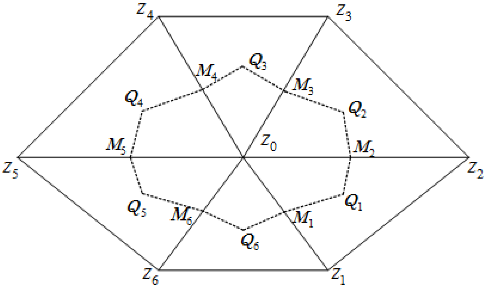
Now, as shown in Figure 1, let ${\mathcal{T}}_h=\left\{K\right\}$ be a quasi-uniform triangular partition of the domain $\Omega$ with $h=max\left\{h_K\right\}$, where $h_K$ is the diameter of the triangular element $K\in {\mathcal{T}}_h$. Then $\overline{\Omega }={\cup }_{K\in T_h}K$ and $Z_h$ denotes all vertices, that is

$$\begin{array}{c}\hfill Z_h=\{z:z\mathrm{is}\mathrm{a}\mathrm{vertex}\mathrm{of}\mathrm{triangular}\mathrm{element}K,K\in T_h\}.\end{array}$$

$Z_h^0\subset Z_h$ denotes the set of interior vertices in ${\mathcal{T}}_h$.

Next, based on the primal partition ${\mathcal{T}}_h$, we construct a dual partition ${\mathcal{T}}_h^{*}$. With $z_0\in Z_h^0$ as an interior node, let $z_j$ $(j=1,2,\cdots ,s)$ be its adjacent nodes (as shown in Figure 1, $s=6$). Let $M_j$ $(j=1,2,\cdots ,s)$ denote the midpoints of $\overline{z_0{z}_j}$ and let $Q_j$ $(j=1,2,\cdots ,s)$ be the barycenters of the triangle $▵z_0{z}_j{z}_{j+1}$ with $z_{n+1}=z_1$. We construct the control volume $K_{z_0}^{*}$ by joining successively $M_1,Q_1,\cdots ,M_s,Q_s,M_1$. With $Q_j,j=1,2,\cdots ,s$ as the nodes of control volume $K_{z_j}^{*}$, let $Z_h^{*}$ be the set of all dual nodes. Then, we construct the dual partition $T_h^{*}$ through the union of all control volumes $K_{z_j}^{*}$.

Then, we define the trial function space $V_h$ and test function space $V_h^{*}$ as follows:

$$\begin{array}{cc}\hfill & V_h=\{v\in H_0^1(\Omega ):v{|}_K\in P_1\left(K\right),\forall K\in {\mathcal{T}}_h\},\hfill \\ \hfill & V_h^{*}=\{v\in L^2{(\Omega ):v|}_{K_z^{*}}\in P_0\left(K_z^{*}\right),\forall K_z^{*}\in {\mathcal{T}}_h^{*},\mathrm{and}v{|}_{\partial \Omega }=0\}.\hfill \end{array}$$

With a node z, let ${\Phi }_z$ be the standard nodal linear basis function, and ${\Psi }_z$ be the characteristic function of the control volume $K_z^{*}$. It is obvious that $V_h=\mathrm{span}\{{\Phi }_z\left(\mathit{x}\right):z\in Z_h^0\}$ and $V_h^{*}=\mathrm{span}\{{\Psi }_z\left(\mathit{x}\right):z\in Z_h^0\}$, We define the piecewise linear interpolation operator $I_h:C(\Omega )\to V_h$ and the piecewise constant interpolation operator $I_h^{*}:C(\Omega )\to V_h^{*}$ as follows:

$$\begin{array}{c}\hfill I_{h}v\left(\mathit{x}\right)=\sum _{z\in Z_h^0}v\left(z\right){\Phi }_z\left(\mathit{x}\right),\mathrm{and}{I}_h^{*}v\left(\mathit{x}\right)=\sum _{z\in Z_h^0}v\left(z\right){\Psi }_z\left(\mathit{x}\right).\end{array}$$

From Reference [30], we can see that $I_h$ and $I_h^{*}$ have the following approximation property

$$\begin{array}{c}\hfill \parallel v-I_h{v\parallel }_j\le C{h}^{2-j}{\parallel v\parallel }_2,j=0,1,\forall v\in H^2(\Omega ),\end{array}$$

(11)

$$\begin{array}{c}\hfill \parallel v-I_h^{*}{v\parallel \le Ch\parallel v\parallel }_1,\forall v\in H^1(\Omega ).\end{array}$$

(12)

Now, integrating (8) over each control volume $K_z^{*}$, and applying the Green formula, we can get

$$\begin{array}{cc}\hfill & {\int }_{K_z^{*}}{\tilde{\partial }}_t{u}^{n+\frac{1}{2}}\mathrm{d}\mathit{x}-{\kappa }_1{\int }_{\partial K_z^{*}}\nabla {\tilde{D}}_{\tau }^{\alpha }{u}^{n+\frac{1}{2}}·\mathit{n}\mathrm{d}s-{\kappa }_2{\int }_{\partial K_z^{*}}\nabla u^{n+\frac{1}{2}}·\mathit{n}\mathrm{d}s\hfill \\ \hfill & ={\int }_{K_z^{*}}f\left(t_{n+\frac{1}{2}}\right)\mathrm{d}\mathit{x}+{\int }_{K_z^{*}}{E}_{\alpha }\left(t_{n+\frac{1}{2}}\right)\mathrm{d}\mathit{x},\forall z\in Z_h,\hfill \end{array}$$

(13)

where $\mathit{n}$ means the outer-normal direction on $\partial K_z^{*}$. Let $u_h\in V_h$ be the discrete solution of u, make use of the operator $I_h^{*}$ to rewrite (13) as the following variational formulation:

$$\begin{array}{cc}\hfill & ({\tilde{\partial }}_t{u}^{n+\frac{1}{2}},I_h^{*}{v}_h)+{\kappa }_{1}a({\tilde{D}}_{\tau }^{\alpha }{u}^{n+\frac{1}{2}},I_h^{*}{v}_h)+{\kappa }_{2}a(u^{n+\frac{1}{2}},I_h^{*}{v}_h)\hfill \\ \hfill & =(f\left(t_{n+\frac{1}{2}}\right),I_h^{*}{v}_h)+(E_{\alpha }\left(t_{n+\frac{1}{2}}\right),I_h^{*}{v}_h),\forall v_h\in V_h,\hfill \end{array}$$

(14)

where the bilinear form $a(·,·)$, following References [30,31], can be rewritten as follows:

$$\begin{array}{c}\hfill a(\overline{u},\overline{v})=\left\{\begin{array}{cc}-\sum _{z\in Z_h}\overline{v}\left(z\right){\int }_{\partial K_z^{*}}\nabla \overline{u}·\mathit{n}\mathrm{d}s,\hfill & \forall \overline{u}\in V_h,\overline{v}\in V_h^{*},\hfill \\ {\int }_{\Omega }\nabla \overline{u}·\nabla \overline{v}\mathrm{d}\mathit{x},\hfill & \forall \overline{u},\overline{v}\in H_0^1(\Omega ).\hfill \end{array}\right.\end{array}$$

(15)

Let $u_h^n$ be the discrete solution of u at $t=t_n$. We establish a fully discrete Crank–Nicolson FVE scheme to seek $u_h^n\in V_h,(n=1,\cdots ,N)$ such that

$$\begin{array}{cc}\hfill & ({\tilde{\partial }}_t{u}_h^{n+\frac{1}{2}},I_h^{*}{v}_h)+{\kappa }_{1}a({\tilde{D}}_{\tau }^{\alpha }{u}_h^{n+\frac{1}{2}},I_h^{*}{v}_h)+{\kappa }_{2}a(u_h^{n+\frac{1}{2}},I_h^{*}{v}_h)\hfill \\ \hfill & =(f\left(t_{n+\frac{1}{2}}\right),I_h^{*}{v}_h),\forall v_h\in V_h,0\le n\le N-1.\hfill \end{array}$$

(16)

And we can rewrite the Crank–Nicolson FVE scheme (16) as the following equivalent formulation:

Case $n=0$:

$$\begin{array}{cc}\hfill & (\frac{u_h^1-u_h^0}{\tau },I_h^{*}{v}_h)+{\kappa }_1\frac{{\tau }^{1-\alpha }}{\tau \Gamma (2-\alpha )}{b}_{0}a(\frac{u_h^1-u_h^0}{2},I_h^{*}{v}_h)+{\kappa }_{2}a(u_h^{\frac{1}{2}},I_h^{*}{v}_h)\hfill \\ \hfill & =(f\left(t_{\frac{1}{2}}\right),I_h^{*}{v}_h),\forall v_h\in V_h.\hfill \end{array}$$

(17)

Case $n\ge 1$:

$$\begin{array}{cc}\hfill & (\frac{u_h^{n+1}-u_h^n}{\tau },I_h^{*}{v}_h)+\frac{{\kappa }_1{\tau }^{1-\alpha }}{\tau \Gamma (2-\alpha )}\sum _{k=0}^{n-1}{b}_{k}a(u_h^{n-k+\frac{1}{2}}-u_h^{n-k-\frac{1}{2}},I_h^{*}{v}_h)\hfill \\ \hfill & +\frac{{\kappa }_1{\tau }^{1-\alpha }}{\tau \Gamma (2-\alpha )}{b}_{n}a(\frac{u_h^1-u_h^0}{2},I_h^{*}{v}_h)+{\kappa }_{2}a(u_h^{n+\frac{1}{2}},I_h^{*}{v}_h)\hfill \\ \hfill & =(f\left(t_{n+\frac{1}{2}}\right),I_h^{*}{v}_h),\forall v_h\in V_h.\hfill \end{array}$$

(18)

Remark 1.

In the construction of the dual partition ${\mathcal{T}}_h^{*}$, we can also choose $Q_j$ as the circumcenter of the triangular element, as shown in Figure 3.2.2 in Reference [30]. Based on this circumcenter dual partition, we can also construct the Crank–Nicolson FVE scheme, and obtain the same theoretical analysis.

Remark 2.

When the barycenter dual partition is selected, there is no essential difference between the structured and unstructured primal partition in the proposed Crank–Nicolson FVE scheme. However, when the circumcenter dual partition is selected and the space domain Ω is rectangular, based on the structured primal partition, the proposed scheme will become more simple, and is similar to the finite difference scheme.

Remark 3.

Making use of Lemmas 1 and 2 in Section 3, we can easily have that the coefficient matrices of linear equations generated by (17) and (18) are invertible. Then, there exists a unique discrete solution for the Crank–Nicolson FVE scheme (16).

3. Stability Analysis

In order to give the stability analysis, we first introduce some properties of the bilinear forms $(·,I_h^{*}·)$ and $a(·,I_h^{*}·)$.

Lemma 1.

[30] The following symmetry relation for the bilinear form $(·,I_h^{*}·)$ holds:

$$\begin{array}{c}\hfill (u_h,I_h^{*}{v}_h)=(v_h,I_h^{*}{u}_h),\forall u_h,v_h\in V_h.\end{array}$$

(19)

Moreover, there exist two positive constants ${\mu }_1$ and ${\mu }_2$ independent of h such that

$$\begin{array}{c}\hfill (u_h,I_h^{*}{u}_h)\ge {\mu }_1{\parallel u_h\parallel }^2,\forall u_h\in V_h,\end{array}$$

(20)

$$\begin{array}{c}\hfill (u_h,I_h^{*}{v}_h)\le {\mu }_2\parallel u_h\parallel \parallel v_h\parallel ,\forall u_h,v_h\in V_h.\end{array}$$

(21)

Lemma 2.

[30] The following symmetry relation for the bilinear form $a(·,I_h^{*}·)$ holds:

$$\begin{array}{c}\hfill a(u_h,I_h^{*}{v}_h)=a(v_h,I_h^{*}{u}_h),\forall u_h,v_h\in V_h.\end{array}$$

(22)

Moreover, there exist two positive constants ${\mu }_3$ and ${\mu }_4$ independent of h such that

$$\begin{array}{c}\hfill a(u_h,I_h^{*}{u}_h)\ge {\mu }_3{\parallel u_h\parallel }_1^2,\forall u_h\in V_h,\end{array}$$

(23)

$$\begin{array}{c}\hfill a(u_h,I_h^{*}{v}_h)\le {\mu }_4\parallel u_h{\parallel }_1{\parallel v_h\parallel }_1,\forall u_h,v_h\in V_h.\end{array}$$

(24)

Next, we give the unconditional stability result for the Crank–Nicolson FVE scheme (16).

Theorem 1.

Let ${\left\{u_h^n\right\}}_{n=1}^N$ be the solutions of the Crank–Nicolson FVE scheme (16), then there exists a positive constant C independent of h and τ such that

$$\begin{array}{c}\hfill \parallel u_h^n\parallel \le C(\parallel u_h^0{\parallel }_1+\underset{t\in [0,T]}{sup}\parallel f\left(t\right)\parallel )\end{array}$$

Proof. 

For the case of $n=0$, choosing $v_h=2u_h^{\frac{1}{2}}=u_h^1+u_h^0$ in (17), we obtain

$$\begin{array}{cc}\hfill & (u_h^1-u_h^0,I_h^{*}(u_h^1+u_h^0))+\frac{2{\kappa }_1{\tau }^{1-\alpha }}{\Gamma (2-\alpha )}{b}_{0}a(u_h^{\frac{1}{2}},I_h^{*}{u}_h^{\frac{1}{2}})+2{\kappa }_2\tau a(u_h^{\frac{1}{2}},I_h^{*}{u}_h^{\frac{1}{2}})\hfill \\ \hfill & =\frac{2{\kappa }_1{\tau }^{1-\alpha }}{\Gamma (2-\alpha )}{b}_{0}a(u_h^0,I_h^{*}{u}_h^{\frac{1}{2}})+2\tau (f\left(t_{\frac{1}{2}}\right),I_h^{*}{u}_h^{\frac{1}{2}}).\hfill \end{array}$$

(25)

Applying Lemma 2, we have

$$\begin{array}{c}\hfill 2a(u_h^0,I_h^{*}{u}_h^{\frac{1}{2}})\le a(u_h^0,I_h^{*}{u}_h^0)+a(u_h^{\frac{1}{2}},I_h^{*}{u}_h^{\frac{1}{2}}).\end{array}$$

(26)

Then, making use of (26) in (25), we obtain

$$\begin{array}{cc}\hfill & (u_h^1,I_h^{*}{u}_h^1)+\frac{{\kappa }_1{\tau }^{1-\alpha }}{\Gamma (2-\alpha )}{b}_{0}a(u_h^{\frac{1}{2}},I_h^{*}{u}_h^{\frac{1}{2}})+2{\kappa }_2\tau a(u_h^{\frac{1}{2}},I_h^{*}{u}_h^{\frac{1}{2}})\hfill \\ \hfill & \le (u_h^0,I_h^{*}{u}_h^0)+\frac{{\kappa }_1{\tau }^{1-\alpha }}{\Gamma (2-\alpha )}{b}_{0}a(u_h^0,I_h^{*}{u}_h^0)+C\tau {\parallel f\left(t_{\frac{1}{2}}\right)\parallel }^2+{\kappa }_2\tau a(u_h^{\frac{1}{2}},I_h^{*}{u}_h^{\frac{1}{2}}).\hfill \end{array}$$

(27)

Applying Lemmas 1 and 2, we obtain

$$\begin{array}{cc}\hfill & (u_h^1,I_h^{*}{u}_h^1)+\frac{{\kappa }_1{\tau }^{1-\alpha }}{\Gamma (2-\alpha )}{b}_{0}a(u_h^{\frac{1}{2}},I_h^{*}{u}_h^{\frac{1}{2}})+{\kappa }_2\tau a(u_h^{\frac{1}{2}},I_h^{*}{u}_h^{\frac{1}{2}})\hfill \\ \hfill & \le {\mu }_2\parallel u_h^0{\parallel }^2+\frac{{\kappa }_1{\tau }^{1-\alpha }}{\Gamma (2-\alpha )}{b}_0{\mu }_4\parallel u_h^0{\parallel }_1^2+C\tau {\parallel f\left(t_{\frac{1}{2}}\right)\parallel }^2.\hfill \end{array}$$

(28)

For the case of $n\ge 1$, choosing $v_h=2u_h^{n+\frac{1}{2}}=u_h^{n+1}+u_h^n$ in (18), we get

$$\begin{array}{cc}\hfill & ((u_h^{n+1}-u_h^n),I_h^{*}(u_h^{n+1}+u_h^n))+\frac{2{\kappa }_1{\tau }^{1-\alpha }}{\Gamma (2-\alpha )}\sum _{k=0}^{n-1}{b}_{k}a(u_h^{n-k+\frac{1}{2}}-u_h^{n-k-\frac{1}{2}},I_h^{*}{u}_h^{n+\frac{1}{2}})\hfill \\ \hfill & +\frac{{\kappa }_1{\tau }^{1-\alpha }}{\Gamma (2-\alpha )}{b}_{n}a(u_h^1-u_h^0,I_h^{*}{u}_h^{n+\frac{1}{2}})+2{\kappa }_2\tau a(u_h^{n+\frac{1}{2}},I_h^{*}{u}_h^{n+\frac{1}{2}})\hfill \\ \hfill & =2\tau (f\left(t_{n+\frac{1}{2}}\right),I_h^{*}{u}_h^{n+\frac{1}{2}}).\hfill \end{array}$$

(29)

Noting that

$$\begin{array}{cc}\hfill & \frac{2{\kappa }_1{\tau }^{1-\alpha }}{\Gamma (2-\alpha )}\sum _{k=0}^{n-1}{b}_{k}a(u_h^{n-k+\frac{1}{2}}-u_h^{n-k-\frac{1}{2}},I_h^{*}{u}_h^{n+\frac{1}{2}})+\frac{{\kappa }_1{\tau }^{1-\alpha }}{\Gamma (2-\alpha )}{b}_{n}a(u_h^1-u_h^0,I_h^{*}{u}_h^{n+\frac{1}{2}})\hfill \\ \hfill & =\frac{2{\kappa }_1{\tau }^{1-\alpha }}{\Gamma (2-\alpha )}\sum _{k=0}^n{b}_{k}a(u_h^{n-k+\frac{1}{2}},I_h^{*}{u}_h^{n+\frac{1}{2}})-\frac{2{\kappa }_1{\tau }^{1-\alpha }}{\Gamma (2-\alpha )}\sum _{k=0}^{n-1}{b}_{k}a(u_h^{n-k-\frac{1}{2}},I_h^{*}{u}_h^{n+\frac{1}{2}})\hfill \\ \hfill & -\frac{2{\kappa }_1{\tau }^{1-\alpha }}{\Gamma (2-\alpha )}{b}_{n}a(u_h^0,I_h^{*}{u}_h^{n+\frac{1}{2}})\hfill \\ \hfill & =\frac{2{\kappa }_1{\tau }^{1-\alpha }}{\Gamma (2-\alpha )}{b}_{0}a(u_h^{n+\frac{1}{2}},I_h^{*}{u}_h^{n+\frac{1}{2}})-\frac{2{\kappa }_1{\tau }^{1-\alpha }}{\Gamma (2-\alpha )}\sum _{k=0}^{n-1}(b_k-b_{k+1})a(u_h^{n-k-\frac{1}{2}},I_h^{*}{u}_h^{n+\frac{1}{2}})\hfill \\ \hfill & -\frac{2{\kappa }_1{\tau }^{1-\alpha }}{\Gamma (2-\alpha )}{b}_{n}a(u_h^0,I_h^{*}{u}_h^{n+\frac{1}{2}}),\hfill \end{array}$$

(30)

and substituting (30) into (29), we obtain

$$\begin{array}{cc}\hfill & ((u_h^{n+1}-u_h^n),I_h^{*}(u_h^{n+1}+u_h^n))+\frac{2{\kappa }_1{\tau }^{1-\alpha }}{\Gamma (2-\alpha )}{b}_{0}a(u_h^{n+\frac{1}{2}},I_h^{*}{u}_h^{n+\frac{1}{2}})+2{\kappa }_2\tau a(u_h^{n+\frac{1}{2}},I_h^{*}{u}_h^{n+\frac{1}{2}})\hfill \\ \hfill & =\frac{2{\kappa }_1{\tau }^{1-\alpha }}{\Gamma (2-\alpha )}\sum _{k=0}^{n-1}(b_k-b_{k+1})a(u_h^{n-k-\frac{1}{2}},I_h^{*}{u}_h^{n+\frac{1}{2}})+\frac{2{\kappa }_1{\tau }^{1-\alpha }}{\Gamma (2-\alpha )}{b}_{n}a(u_h^0,I_h^{*}{u}_h^{n+\frac{1}{2}})\hfill \\ \hfill & +2\tau (f\left(t_{n+\frac{1}{2}}\right),I_h^{*}{u}_h^{n+\frac{1}{2}}).\hfill \end{array}$$

(31)

Applying Lemma 2, we have

$$\begin{array}{cc}\hfill 2a(u_h^{n-k-\frac{1}{2}},I_h^{*}{u}_h^{n+\frac{1}{2}})& \le a(u_h^{n-k-\frac{1}{2}},I_h^{*}{u}_h^{n-k-\frac{1}{2}})+a(u_h^{n+\frac{1}{2}},I_h^{*}{u}_h^{n+\frac{1}{2}}),\hfill \end{array}$$

(32)

and

$$\begin{array}{cc}\hfill 2a(u_h^0,I_h^{*}{u}_h^{n+\frac{1}{2}})& \le a(u_h^0,I_h^{*}{u}_h^0)+a(u_h^{n+\frac{1}{2}},I_h^{*}{u}_h^{n+\frac{1}{2}}).\hfill \end{array}$$

(33)

Noting that $b_k-b_{k+1}=-{(k+2)}^{1-\alpha }+2k^{1-\alpha }-{(k-1)}^{1-\alpha }>0$, and substituting (32) and (33) into (31), we have

$$\begin{array}{cc}\hfill & (u_h^{n+1},I_h^{*}{u}_h^{n+1})+\frac{{\kappa }_1{\tau }^{1-\alpha }}{\Gamma (2-\alpha )}\sum _{k=0}^n{b}_{k}a(u_h^{n-k+\frac{1}{2}},I_h^{*}{u}_h^{n-k+\frac{1}{2}})+2{\kappa }_2\tau a(u_h^{n+\frac{1}{2}},I_h^{*}{u}_h^{n+\frac{1}{2}})\hfill \\ \hfill & \le (u_h^n,I_h^{*}{u}_h^n)+\frac{{\kappa }_1{\tau }^{1-\alpha }}{\Gamma (2-\alpha )}\sum _{k=0}^{n-1}{b}_{k}a(u_h^{n-k-\frac{1}{2}},I_h^{*}{u}_h^{n-k-\frac{1}{2}})\hfill \\ \hfill & +\frac{{\kappa }_1{\tau }^{1-\alpha }}{\Gamma (2-\alpha )}{b}_{n}a(u_h^0,I_h^{*}{u}_h^0)+2\tau (f\left(t_{n+\frac{1}{2}}\right),I_h^{*}{u}_h^{n+\frac{1}{2}}).\hfill \end{array}$$

(34)

Apply Lemma 2 and the Young inequality to obtain

$$\begin{array}{cc}\hfill & (u_h^{n+1},I_h^{*}{u}_h^{n+1})+\frac{{\kappa }_1{\tau }^{1-\alpha }}{\Gamma (2-\alpha )}\sum _{k=0}^n{b}_{k}a(u_h^{n-k+\frac{1}{2}},I_h^{*}{u}_h^{n-k+\frac{1}{2}})+{\kappa }_2{\mu }_3\tau {\parallel u_h^{n+\frac{1}{2}}\parallel }_1^2\hfill \\ \hfill & \le (u_h^n,I_h^{*}{u}_h^n)+\frac{{\kappa }_1{\tau }^{1-\alpha }}{\Gamma (2-\alpha )}\sum _{k=0}^{n-1}{b}_{k}a(u_h^{n-k-\frac{1}{2}},I_h^{*}{u}_h^{n-k-\frac{1}{2}})+{\kappa }_2{\mu }_3\tau {\parallel u_h^{n-\frac{1}{2}}\parallel }_1^2\hfill \\ \hfill & +\frac{{\kappa }_1{\tau }^{1-\alpha }}{\Gamma (2-\alpha )}{b}_n{\mu }_4\parallel u_h^0{\parallel }_1^2+C\tau {\parallel f\left(t_{n+\frac{1}{2}}\right)\parallel }^2.\hfill \end{array}$$

(35)

Now, let ${\Lambda }^n=(u_h^n,I_h^{*}{u}_h^n)+\frac{{\kappa }_1{\tau }^{1-\alpha }}{\Gamma (2-\alpha )}{\sum }_{k=0}^{n-1}{b}_{k}a(u_h^{n-k-\frac{1}{2}},I_h^{*}{u}_h^{n-k-\frac{1}{2}})+{\kappa }_2{\mu }_3\tau {\parallel u_h^{n-\frac{1}{2}}\parallel }_1^2$. We can rewrite (35) as follows:

$$\begin{array}{c}\hfill {\Lambda }^{n+1}\le {\Lambda }^n+\frac{{\kappa }_1{\tau }^{1-\alpha }}{\Gamma (2-\alpha )}{b}_n{\mu }_4\parallel u_h^0{\parallel }_1^2+C\tau {\parallel f\left(t_{n+\frac{1}{2}}\right)\parallel }^2\end{array}$$

(36)

By using the direct recursive method in (36), we have

$$\begin{array}{c}\hfill {\Lambda }^{n+1}\le {\Lambda }^1+\frac{{\kappa }_1{\tau }^{1-\alpha }}{\Gamma (2-\alpha )}\left(\sum _{k=1}^n{b}_k\right){\mu }_4\parallel u_h^0{\parallel }_1^2+Cn\tau \underset{t\in [0,T]}{sup}{\parallel f\left(t\right)\parallel }^2.\end{array}$$

(37)

Making use of (28), we estimate ${\Lambda }^1$ as follows:

$$\begin{array}{c}\hfill {\Lambda }^1\le {\mu }_2\parallel u_h^0{\parallel }^2+\frac{{\kappa }_1{\tau }^{1-\alpha }}{\Gamma (2-\alpha )}{b}_0{\mu }_4\parallel u_h^0{\parallel }_1^2+C\tau {\parallel f\left(t_{\frac{1}{2}}\right)\parallel }^2.\end{array}$$

(38)

Substituting (38) into (37), we have

$$\begin{array}{cc}\hfill {\Lambda }^{n+1}& \le {\mu }_2\parallel u_h^0{\parallel }^2+\frac{{\kappa }_1{\tau }^{1-\alpha }}{\Gamma (2-\alpha )}\left(\sum _{k=0}^n{b}_k\right){\mu }_4\parallel u_h^0{\parallel }_1^2+C(n+1)\tau \underset{t\in [0,T]}{sup}{\parallel f\left(t\right)\parallel }^2\hfill \\ \hfill & ={\mu }_2\parallel u_h^0{\parallel }^2+\frac{{\kappa }_1{\tau }^{1-\alpha }}{\Gamma (2-\alpha )}{(n+1)}^{1-\alpha }{\mu }_4\parallel u_h^0{\parallel }_1^2+C(n+1)\tau \underset{t\in [0,T]}{sup}{\parallel f\left(t\right)\parallel }^2\hfill \\ \hfill & \le {\mu }_2\parallel u_h^0{\parallel }^2+\frac{{\kappa }_1{\mu }_4{T}^{1-\alpha }}{\Gamma (2-\alpha )}\parallel u_h^0{\parallel }_1^2+CT\underset{t\in [0,T]}{sup}{\parallel f\left(t\right)\parallel }^2.\hfill \end{array}$$

(39)

Thus, apply the definition of ${\Lambda }^n$ and Lemma 1 to complete the proof. □

4. Convergence Analysis

In order to obtain the error estimates for the Crank–Nicolson FVE scheme (16), we need to introduce a projection operator $P_h:$ $H_0^1(\Omega )\cap H^2(\Omega )\to V_h$, which is defined by the following formulation:

$$\begin{array}{c}\hfill a(u-P_{h}u,I_h^{*}{v}_h)=0,\forall v_h\in V_h.\end{array}$$

(40)

Following Reference [30], we give the following estimates for the projection operator $P_h$.

Lemma 3.

There exists a positive constant C independent of h and τ such that

$$\begin{array}{c}\hfill \parallel u-P_h{u\parallel }_1\le Ch{\left|u\right|}_2,\forall u\in H_0^1(\Omega )\cap H^2(\Omega ),\end{array}$$

(41)

$$\begin{array}{c}\hfill \parallel u-P_{h}u\parallel \le C{h}^2{\parallel u\parallel }_{3,p},\forall u\in H_0^1(\Omega )\cap W^{3,p}(\Omega ),p>1.\end{array}$$

(42)

Next, we give the optimal a priori error estimate for the Crank–Nicolson FVE scheme (16).

Theorem 2.

Let $u\left(t_n\right)$ and $u_h^n$ be the solutions of system (14) and the Crank–Nicolson FVE scheme (16), respectively, $u_h^0=P_h{u}_0$, $u\in {\mathcal{C}}^2(\overline{J},H_0^1(\Omega )\cap W^{3,p}(\Omega )),p>1$, and $u_{ttt}\in L^{\infty }(\overline{J},L^2(\Omega ))$, then there exists a positive constant C independent of h and τ such that

$$\begin{array}{c}\hfill \underset{1\le n\le N}{max}\parallel u\left(t_n\right)-u_h^n\parallel \le C({\tau }^{2-\alpha }+h^2).\end{array}$$

Proof. 

We split the error as follows:

$$\begin{array}{c}\hfill u\left(t_n\right)-u_h^n=u\left(t_n\right)-P_{h}u\left(t_n\right)+P_{h}u\left(t_n\right)-u_h^n={\eta }^n+{\xi }^n.\end{array}$$

(43)

According to Lemma 3, it is only necessary to estimate ${\xi }^n$. Making using of our definitions, we can get the error equation of ${\xi }^n$. For the case of $n=0$, we have

$$\begin{array}{cc}\hfill & ({\xi }^1-{\xi }^0,I_h^{*}{v}_h)+\frac{{\kappa }_1{\tau }^{1-\alpha }}{\Gamma (2-\alpha )}\frac{b_0}{2}a({\xi }^1-{\xi }^0,I_h^{*}{v}_h)+{\kappa }_2\tau a({\xi }^{\frac{1}{2}},I_h^{*}{v}_h)\hfill \\ \hfill & =-({\eta }^1-{\eta }^0,I_h^{*}{v}_h)+\tau (E_{\alpha }\left(t_{\frac{1}{2}}\right),I_h^{*}{v}_h),\forall v_h\in V_h.\hfill \end{array}$$

(44)

For the case of $n\ge 1$, we have

$$\begin{array}{cc}\hfill & ({\xi }^{n+1}-{\xi }^n,I_h^{*}{v}_h)+\frac{{\kappa }_1{\tau }^{1-\alpha }}{\Gamma (2-\alpha )}\sum _{k=0}^{n-1}{b}_{k}a({\xi }^{n-k+\frac{1}{2}}-{\xi }^{n-k-\frac{1}{2}},I_h^{*}{v}_h)\hfill \\ \hfill & +\frac{{\kappa }_1{\tau }^{1-\alpha }}{\Gamma (2-\alpha )}\frac{b_n}{2}a({\xi }^1-{\xi }^0,I_h^{*}{v}_h)+{\kappa }_2\tau a({\xi }^{n+\frac{1}{2}},I_h^{*}{v}_h)\hfill \\ \hfill & =-({\eta }^{n+1}-{\eta }^n,I_h^{*}{v}_h)+\tau (E_{\alpha }\left(t_{n+\frac{1}{2}}\right),I_h^{*}{v}_h),\forall v_h\in V_h.\hfill \end{array}$$

(45)

Next, choosing $v_h={\xi }^1=2{\xi }^{\frac{1}{2}}$ in (44), and noting that ${\xi }^0=0$, we obtain

$$\begin{array}{cc}\hfill & ({\xi }^1,I_h^{*}{\xi }^1)+\frac{2{\kappa }_1{\tau }^{1-\alpha }}{\Gamma (2-\alpha )}{b}_{0}a({\xi }^{\frac{1}{2}},I_h^{*}{\xi }^{\frac{1}{2}})+2{\kappa }_2\tau a({\xi }^{\frac{1}{2}},I_h^{*}{\xi }^{\frac{1}{2}})\hfill \\ \hfill & =-2\tau ({\partial }_t{\eta }^{\frac{1}{2}},I_h^{*}{\xi }^{\frac{1}{2}})+2\tau (E_{\alpha }\left(t_{\frac{1}{2}}\right),I_h^{*}{\xi }^{\frac{1}{2}}),\hfill \end{array}$$

(46)

Apply Lemma 1 and the Young inequality to obtain

$$\begin{array}{cc}\hfill & ({\xi }^1,I_h^{*}{\xi }^1)+\frac{2{\kappa }_1{\tau }^{1-\alpha }}{\Gamma (2-\alpha )}{b}_{0}a({\xi }^{\frac{1}{2}},I_h^{*}{\xi }^{\frac{1}{2}})+2{\kappa }_2\tau a({\xi }^{\frac{1}{2}},I_h^{*}{\xi }^{\frac{1}{2}})\hfill \\ \hfill & \le C\tau (\parallel {\partial }_t{\eta }^{\frac{1}{2}}{\parallel }^2+\parallel E_{\alpha }\left(t_{\frac{1}{2}}\right){\parallel }^2)+{\kappa }_2\tau a({\xi }^{\frac{1}{2}},I_h^{*}{\xi }^{\frac{1}{2}}).\hfill \end{array}$$

(47)

Noting that

$$\begin{array}{c}\hfill \parallel {\partial }_t{\eta }^{\frac{1}{2}}{\parallel }^2=\parallel \frac{1}{\tau }{\int }_{t_0}^{t_1}{\eta }_t{\mathrm{d}t\parallel }^2\le C{h}^4{\parallel u_t\parallel }_{L^{\infty }\left(W^{3,p}\right)}^2,p>1,\end{array}$$

(48)

and making use of the truncation error of $E_{\alpha }\left(t_{n+\frac{1}{2}}\right)$, we have

$$\begin{array}{cc}\hfill & ({\xi }^1,I_h^{*}{\xi }^1)+\frac{2{\kappa }_1{\tau }^{1-\alpha }}{\Gamma (2-\alpha )}{b}_{0}a({\xi }^{\frac{1}{2}},I_h^{*}{\xi }^{\frac{1}{2}})+{\kappa }_2\tau a({\xi }^{\frac{1}{2}},I_h^{*}{\xi }^{\frac{1}{2}})\hfill \\ \hfill & \le C\tau ({({\tau }^2+{\tau }^{2-\alpha })}^2+h^4).\hfill \end{array}$$

(49)

Now, choosing $v_h=2{\xi }^{n+\frac{1}{2}}={\xi }^n+{\xi }^{n+1}$ in (45), we get

$$\begin{array}{cc}\hfill & ({\xi }^{n+1}-{\xi }^n,I_h^{*}({\xi }^n+{\xi }^{n+1}))+\frac{2{\kappa }_1{\tau }^{1-\alpha }}{\Gamma (2-\alpha )}\sum _{k=0}^{n-1}{b}_{k}a({\xi }^{n-k+\frac{1}{2}}-{\xi }^{n-k-\frac{1}{2}},I_h^{*}{\xi }^{n+\frac{1}{2}})\hfill \\ \hfill & +\frac{2{\kappa }_1{\tau }^{1-\alpha }}{\Gamma (2-\alpha )}{b}_{n}a({\xi }^{\frac{1}{2}},I_h^{*}{\xi }^{n+\frac{1}{2}})+2{\kappa }_2\tau a({\xi }^{n+\frac{1}{2}},I_h^{*}{\xi }^{n+\frac{1}{2}})\hfill \\ \hfill & =-2({\eta }^{n+1}-{\eta }^n,I_h^{*}{\xi }^{n+\frac{1}{2}})+2\tau (E_{\alpha }\left(t_{n+\frac{1}{2}}\right),I_h^{*}{\xi }^{n+\frac{1}{2}}).\hfill \end{array}$$

(50)

Noting that ${\xi }^0=0$, we have

$$\begin{array}{cc}\hfill & \frac{2{\kappa }_1{\tau }^{1-\alpha }}{\Gamma (2-\alpha )}\sum _{k=0}^{n-1}{b}_{k}a({\xi }^{n-k+\frac{1}{2}}-{\xi }^{n-k-\frac{1}{2}},I_h^{*}{\xi }^{n+\frac{1}{2}})+\frac{2{\kappa }_1{\tau }^{1-\alpha }}{\Gamma (2-\alpha )}{b}_{n}a({\xi }^{\frac{1}{2}},I_h^{*}{\xi }^{n+\frac{1}{2}})\hfill \\ \hfill & =\frac{2{\kappa }_1{\tau }^{1-\alpha }}{\Gamma (2-\alpha )}{b}_{0}a({\xi }^{n+\frac{1}{2}},I_h^{*}{\xi }^{n+\frac{1}{2}})+\frac{2{\kappa }_1{\tau }^{1-\alpha }}{\Gamma (2-\alpha )}\sum _{k=1}^n{b}_{k}a({\xi }^{n-k+\frac{1}{2}},I_h^{*}{\xi }^{n+\frac{1}{2}})\hfill \\ \hfill & -\frac{2{\kappa }_1{\tau }^{1-\alpha }}{\Gamma (2-\alpha )}\sum _{k=0}^{n-1}{b}_{k}a({\xi }^{n-k-\frac{1}{2}},I_h^{*}{\xi }^{n+\frac{1}{2}})\hfill \\ \hfill & =\frac{2{\kappa }_1{\tau }^{1-\alpha }}{\Gamma (2-\alpha )}{b}_{0}a({\xi }^{n+\frac{1}{2}},I_h^{*}{\xi }^{n+\frac{1}{2}})-\frac{2{\kappa }_1{\tau }^{1-\alpha }}{\Gamma (2-\alpha )}\sum _{k=0}^{n-1}(b_k-b_{k+1})a({\xi }^{n-k-\frac{1}{2}},I_h^{*}{\xi }^{n+\frac{1}{2}}).\hfill \end{array}$$

(51)

Substituting (51) into (50), we obtain

$$\begin{array}{cc}\hfill & ({\xi }^{n+1}-{\xi }^n,I_h^{*}({\xi }^n+{\xi }^{n+1}))+\frac{2{\kappa }_1{\tau }^{1-\alpha }}{\Gamma (2-\alpha )}{b}_{0}a({\xi }^{n+\frac{1}{2}},I_h^{*}{\xi }^{n+\frac{1}{2}})+2{\kappa }_2\tau a({\xi }^{n+\frac{1}{2}},I_h^{*}{\xi }^{n+\frac{1}{2}})\hfill \\ \hfill & =\frac{2{\kappa }_1{\tau }^{1-\alpha }}{\Gamma (2-\alpha )}\sum _{k=0}^{n-1}(b_k-b_{k+1})a({\xi }^{n-k-\frac{1}{2}},I_h^{*}{\xi }^{n+\frac{1}{2}})-2\tau ({\partial }_t{\eta }^{n+\frac{1}{2}},I_h^{*}{\xi }^{n+\frac{1}{2}})\hfill \\ \hfill & +2\tau (E_{\alpha }\left(t_{n+\frac{1}{2}}\right),I_h^{*}{\xi }^{n+\frac{1}{2}}).\hfill \end{array}$$

(52)

Noting that $b_k-b_{k+1}>0$ and $2a({\xi }^{n-k-\frac{1}{2}},I_h^{*}{\xi }^{n+\frac{1}{2}})\le a({\xi }^{n-k-\frac{1}{2}},I_h^{*}{\xi }^{n-k-\frac{1}{2}})+a({\xi }^{n+\frac{1}{2}},I_h^{*}{\xi }^{n+\frac{1}{2}})$, we have

$$\begin{array}{cc}\hfill & \frac{2{\kappa }_1{\tau }^{1-\alpha }}{\Gamma (2-\alpha )}\sum _{k=0}^{n-1}(b_k-b_{k+1})a({\xi }^{n-k-\frac{1}{2}},I_h^{*}{\xi }^{n+\frac{1}{2}})\hfill \\ \hfill & \le \frac{{\kappa }_1{\tau }^{1-\alpha }}{\Gamma (2-\alpha )}\sum _{k=0}^{n-1}(b_k-b_{k+1})a({\xi }^{n-k-\frac{1}{2}},I_h^{*}{\xi }^{n-k-\frac{1}{2}})\hfill \\ \hfill & +\frac{{\kappa }_1{\tau }^{1-\alpha }}{\Gamma (2-\alpha )}(b_0-b_n)a({\xi }^{n+\frac{1}{2}},I_h^{*}{\xi }^{n+\frac{1}{2}}).\hfill \end{array}$$

(53)

Substituting (53) into (52), we can get

$$\begin{array}{cc}\hfill & ({\xi }^{n+1},I_h^{*}{\xi }^{n+1})+\frac{{\kappa }_1{\tau }^{1-\alpha }}{\Gamma (2-\alpha )}\sum _{k=0}^n{b}_{k}a({\xi }^{n-k+\frac{1}{2}},I_h^{*}{\xi }^{n-k+\frac{1}{2}})\hfill \\ \hfill & +2{\kappa }_2\tau a({\xi }^{n+\frac{1}{2}},I_h^{*}{\xi }^{n+\frac{1}{2}})+\frac{{\kappa }_1{\tau }^{1-\alpha }}{\Gamma (2-\alpha )}{b}_{n}a({\xi }^{n+\frac{1}{2}},I_h^{*}{\xi }^{n+\frac{1}{2}})\hfill \\ \hfill & \le ({\xi }^n,I_h^{*}{\xi }^n)+\frac{{\kappa }_1{\tau }^{1-\alpha }}{\Gamma (2-\alpha )}\sum _{k=0}^{n-1}{b}_{k}a({\xi }^{n-k-\frac{1}{2}},I_h^{*}{\xi }^{n-k-\frac{1}{2}})\hfill \\ \hfill & -2\tau ({\partial }_t{\eta }^{n+\frac{1}{2}},I_h^{*}{\xi }^{n+\frac{1}{2}})+2\tau (E_{\alpha }\left(t_{n+\frac{1}{2}}\right),I_h^{*}{\xi }^{n+\frac{1}{2}}).\hfill \end{array}$$

(54)

Applying the Cauchy–Schwarz inequality and Young inequality in (54), we derive

$$\begin{array}{cc}\hfill & ({\xi }^{n+1},I_h^{*}{\xi }^{n+1})+\frac{{\kappa }_1{\tau }^{1-\alpha }}{\Gamma (2-\alpha )}\sum _{k=0}^n{b}_{k}a({\xi }^{n-k+\frac{1}{2}},I_h^{*}{\xi }^{n-k+\frac{1}{2}})\hfill \\ \hfill & +{\kappa }_2{\mu }_3\tau {\parallel {\xi }^{n+\frac{1}{2}}\parallel }_1^2+\frac{{\kappa }_1{\tau }^{1-\alpha }}{\Gamma (2-\alpha )}{b}_{n}a({\xi }^{n+\frac{1}{2}},I_h^{*}{\xi }^{n+\frac{1}{2}})\hfill \\ \hfill & \le ({\xi }^n,I_h^{*}{\xi }^n)+\frac{{\kappa }_1{\tau }^{1-\alpha }}{\Gamma (2-\alpha )}\sum _{k=0}^{n-1}{b}_{k}a({\xi }^{n-k-\frac{1}{2}},I_h^{*}{\xi }^{n-k-\frac{1}{2}})\hfill \\ \hfill & +C\tau (\parallel {\partial }_t{\eta }^{n+\frac{1}{2}}{\parallel }^2+\parallel E_{\alpha }\left(t_{n+\frac{1}{2}}\right){\parallel }^2).\hfill \end{array}$$

(55)

Noting that

$$\begin{array}{c}\hfill \parallel {\partial }_t{\eta }^{n+\frac{1}{2}}{\parallel }^2=\parallel \frac{1}{\tau }{\int }_{t_n}^{t_{n+1}}{\rho }_t{\mathrm{d}t\parallel }^2\le C{h}^4{\parallel u_t\parallel }_{L^{\infty }\left(W^{3,p}\right)}^2,p>1,\end{array}$$

(56)

and substituting (56) into (55), we have

$$\begin{array}{cc}\hfill & ({\xi }^{n+1},I_h^{*}{\xi }^{n+1})+\frac{{\kappa }_1{\tau }^{1-\alpha }}{\Gamma (2-\alpha )}\sum _{k=0}^n{b}_{k}a({\xi }^{n-k+\frac{1}{2}},I_h^{*}{\xi }^{n-k+\frac{1}{2}})\hfill \\ \hfill & +{\kappa }_2{\mu }_3\tau {\parallel {\xi }^{n+\frac{1}{2}}\parallel }_1^2+\frac{{\kappa }_1{\tau }^{1-\alpha }}{\Gamma (2-\alpha )}{b}_{n}a({\xi }^{n+\frac{1}{2}},I_h^{*}{\xi }^{n+\frac{1}{2}})\hfill \\ \hfill & \le ({\xi }^n,I_h^{*}{\xi }^n)+\frac{{\kappa }_1{\tau }^{1-\alpha }}{\Gamma (2-\alpha )}\sum _{k=0}^{n-1}{b}_{k}a({\xi }^{n-k-\frac{1}{2}},I_h^{*}{\xi }^{n-k-\frac{1}{2}})\hfill \\ \hfill & +{\kappa }_2{\mu }_3\tau {\parallel {\xi }^{n-\frac{1}{2}}\parallel }_1^2+C\tau ({({\tau }^2+{\tau }^{2-\alpha })}^2+h^4).\hfill \end{array}$$

(57)

Thus, we define ${\Lambda }_h^n$ as follows:

$$\begin{array}{c}\hfill {\Lambda }_h^n=({\xi }^n,I_h^{*}{\xi }^n)+\frac{{\kappa }_1{\tau }^{1-\alpha }}{\Gamma (2-\alpha )}\sum _{k=0}^{n-1}{b}_{k}a({\xi }^{n-k-\frac{1}{2}},I_h^{*}{\xi }^{n-k-\frac{1}{2}})+{\kappa }_2{\mu }_3\tau {\parallel {\xi }^{n-\frac{1}{2}}\parallel }_1^2.\end{array}$$

(58)

Then, making use of (58) and the direct recursive method in (57), we derive

$$\begin{array}{c}\hfill {\Lambda }_h^{n+1}\le {\Lambda }_h^1+Cn\tau ({({\tau }^2+{\tau }^{2-\alpha })}^2+h^4).\end{array}$$

(59)

With the help of (49), we get

$$\begin{array}{cc}\hfill {\Lambda }_h^1& =({\xi }^1,I_h^{*}{\xi }^1)+\frac{{\kappa }_1{\tau }^{1-\alpha }}{\Gamma (2-\alpha )}{b}_{0}a({\xi }^{\frac{1}{2}},I_h^{*}{\xi }^{\frac{1}{2}})+{\kappa }_2{\mu }_3\tau {\parallel {\xi }^{\frac{1}{2}}\parallel }_1^2\hfill \\ \hfill & \le C\tau ({({\tau }^2+{\tau }^{2-\alpha })}^2+h^4).\hfill \end{array}$$

(60)

Substituting (60) into (59), we obtain

$$\begin{array}{c}\hfill {\Lambda }_h^{n+1}\le C(n+1)\tau ({({\tau }^2+{\tau }^{2-\alpha })}^2+h^4)\le CT({({\tau }^2+{\tau }^{2-\alpha })}^2+h^4).\end{array}$$

(61)

Finally, apply the triangle inequality, Lemmas 1 and 3 to complete the proof. □

5. Numerical Examples

In this section, we will give some numerical results to examine the feasibility and effectiveness of the proposed Crank–Nicolson FVE scheme.

Example 1.

We consider the following time fractional Sobolev equation:

$$\begin{array}{c}\hfill \left\{\begin{array}{cc}{\displaystyle \frac{\partial u(\mathit{x},t)}{\partial t}}-{\kappa }_1{\displaystyle \frac{{\partial }^{\alpha }\Delta u(\mathit{x},t)}{\partial t^{\alpha }}}-{\kappa }_2\Delta u(\mathit{x},t)=f(\mathit{x},t),\hfill & (\mathit{x},t)\in \Omega \times J,\hfill \\ u(\mathit{x},t)=0,\hfill & (\mathit{x},t)\in \partial \Omega \times \overline{J},\hfill \\ u(\mathit{x},0)=0,\hfill & \mathit{x}\in \overline{\Omega },\hfill \end{array}\right.\end{array}$$

(62)

where ${\kappa }_1={\kappa }_2=1$, $\Omega =(0,1)\times (0,1)$ and $J=(0,1]$. We choose the source function $f(\mathit{x},t)$ as follows:

$$\begin{array}{cc}\hfill f(\mathit{x},t)=& -(\frac{2t^{2-\alpha }}{\Gamma (3-\alpha )}+t^2)((12x_1^2-12x_1+2){(x_2^2-x_2)}^2+(12x_2^2-12x_2+2){(x_1^2-x_1)}^2)\hfill \\ \hfill & +2t{(x_1^2-x_1)}^2{(x_2^2-x_2)}^2,\forall \mathit{x}=(x_1,x_2)\in \overline{\Omega }.\hfill \end{array}$$

Thus, we can obtain the corresponding exact solution

$$u(\mathit{x},t)=t^2{(x_1^2-x_1)}^2{(x_2^2-x_2)}^2,\forall \mathit{x}=(x_1,x_2)\in \overline{\Omega }.$$

In the actual numerical calculation, in order to reduce the influence of numerical integration on the calculation accuracy as much as possible, we use the composite fifth-order Gauss quadrature formula in triangular domain to calculate some definite integral of space variable, including the calculation of the error $\parallel u\left(t_n\right)-u_h^n\parallel$. In

Table 1. Error $\underset{n}{max}\parallel u\left(t_n\right)-u_h^n\parallel$ with $h=\frac{\sqrt{2}}{160}$ for Example 1.

$\mathit{\alpha }$	${\mathit{\tau }}_1=1/10$	${\mathit{\tau }}_2=1/20$	${\mathit{\tau }}_3=1/40$	Rate ($\frac{{\mathit{\tau }}_1}{{\mathit{\tau }}_2}$)	Rate ($\frac{{\mathit{\tau }}_2}{{\mathit{\tau }}_3}$)
0.1	5.20327276 $\times {10}^{-6}$	1.02981026 $\times {10}^{-6}$	2.57061784 $\times {10}^{-7}$	2.33704079	2.00219149
0.3	4.22066107 $\times {10}^{-6}$	8.81382205 $\times {10}^{-7}$	2.57191087 $\times {10}^{-7}$	2.25962931	1.77692712
0.5	8.41173598 $\times {10}^{-6}$	3.42482403 $\times {10}^{-6}$	1.34374442 $\times {10}^{-6}$	1.29637371	1.34977110
0.7	2.59370022 $\times {10}^{-5}$	1.11771185 $\times {10}^{-5}$	4.73089107 $\times {10}^{-6}$	1.21446343	1.24036446
0.9	6.23406687 $\times {10}^{-5}$	3.00618054 $\times {10}^{-5}$	1.42948701 $\times {10}^{-5}$	1.05224198	1.07243414

, for the fixed space step $h=\sqrt{2}/160$, we choose different fractional parameters $\alpha =0.1,0.3,0.5,0.7,0.9$ and time step $\tau =1/10,1/20,1/40$, and get the corresponding error results. From these results, it is easy to see that the time convergence rates in $L^2(\Omega )$-norm are close to $2-\alpha$ on the whole, which is a little higher when $\alpha =0.1,0.3$ and a little lower when $\alpha =0.5,0.7,0.9$. In

Table 2. Error $\underset{n}{max}\parallel u\left(t_n\right)-u_h^n\parallel$ with $\tau =\frac{1}{1000}$ for Example 1.

$\mathit{\alpha }$	${\mathit{h}}_1=\sqrt{2}/10$	${\mathit{h}}_2=\sqrt{2}/20$	${\mathit{h}}_3=\sqrt{2}/40$	Rate ($\frac{{\mathit{h}}_1}{{\mathit{h}}_2}$)	Rate ($\frac{{\mathit{h}}_2}{{\mathit{h}}_3}$)
0.1	4.65199982 $\times {10}^{-5}$	1.16219022 $\times {10}^{-5}$	2.88479822 $\times {10}^{-6}$	2.00100482	2.01030390
0.3	4.65269409 $\times {10}^{-5}$	1.16237896 $\times {10}^{-5}$	2.88519293 $\times {10}^{-6}$	2.00098584	2.01034080
0.5	4.65340047 $\times {10}^{-5}$	1.16252589 $\times {10}^{-5}$	2.88503002 $\times {10}^{-6}$	2.00102250	2.01060461
0.7	4.65396329 $\times {10}^{-5}$	1.16239089 $\times {10}^{-5}$	2.88231022 $\times {10}^{-6}$	2.00136453	2.01179778
0.9	4.65349753 $\times {10}^{-5}$	1.16120359 $\times {10}^{-5}$	2.88933056 $\times {10}^{-6}$	2.00269450	2.00681377

, we select the same fractional parameters $\alpha$ and different meshes with $h=\sqrt{2}/10,\sqrt{2}/20,\sqrt{2}/40$ and time step $\tau =1/1000$, and get the space convergence rates, which are close to 2. These numerical results are consistent with the theoretical analysis.

Furthermore, we give the error results at different time points $t=0,0.1,0.2,\cdots ,1$. In

Table 3. Errors in $L^2$-norm with $\tau =\frac{1}{1000}$ and $\alpha =0.1$ for Example 1.

t	${\mathit{h}}_1=\sqrt{2}/10$	${\mathit{h}}_2=\sqrt{2}/20$	${\mathit{h}}_3=\sqrt{2}/40$
0	0	0	0
0.1	4.54085533 $\times {10}^{-7}$	1.13055892 $\times {10}^{-7}$	2.80440769 $\times {10}^{-8}$
0.2	1.83951354 $\times {10}^{-6}$	4.58810496 $\times {10}^{-7}$	1.13833634 $\times {10}^{-7}$
0.3	4.15796044 $\times {10}^{-6}$	1.03775203 $\times {10}^{-6}$	2.57514691 $\times {10}^{-7}$
0.4	7.40962070 $\times {10}^{-6}$	1.84993413 $\times {10}^{-6}$	4.59099721 $\times {10}^{-7}$
0.5	1.15945775 $\times {10}^{-5}$	2.89538007 $\times {10}^{-6}$	7.18594459 $\times {10}^{-7}$
0.6	1.67128776 $\times {10}^{-5}$	4.17410301 $\times {10}^{-6}$	1.03600221 $\times {10}^{-6}$
0.7	2.27645513 $\times {10}^{-5}$	5.68611145 $\times {10}^{-6}$	1.41132512 $\times {10}^{-6}$
0.8	2.97496194 $\times {10}^{-5}$	7.43141136 $\times {10}^{-6}$	1.84456472 $\times {10}^{-6}$
0.9	3.76680978 $\times {10}^{-5}$	9.41000714 $\times {10}^{-6}$	2.33572213 $\times {10}^{-6}$
1	4.65199982 $\times {10}^{-5}$	1.16219022 $\times {10}^{-5}$	2.88479822 $\times {10}^{-6}$

and

Table 4. Errors in $L^2$-norm with $\tau =\frac{1}{1000}$ and $\alpha =0.9$ for Example 1.

t	${\mathit{h}}_1=\sqrt{2}/10$	${\mathit{h}}_2=\sqrt{2}/20$	${\mathit{h}}_3=\sqrt{2}/40$
0	0	0	0
0.1	4.67366765 $\times {10}^{-7}$	1.36272751 $\times {10}^{-7}$	8.28616406 $\times {10}^{-8}$
0.2	1.85776832 $\times {10}^{-6}$	4.76415112 $\times {10}^{-7}$	1.76100707 $\times {10}^{-7}$
0.3	4.18008648 $\times {10}^{-6}$	1.05061482 $\times {10}^{-6}$	3.12845166 $\times {10}^{-7}$
0.4	7.43425411 $\times {10}^{-6}$	1.85885698 $\times {10}^{-6}$	5.04807743 $\times {10}^{-7}$
0.5	1.16203815 $\times {10}^{-5}$	2.90081331 $\times {10}^{-6}$	7.55111948 $\times {10}^{-7}$
0.6	1.67386056 $\times {10}^{-5}$	4.17630073 $\times {10}^{-6}$	1.06436272 $\times {10}^{-6}$
0.7	2.27890600 $\times {10}^{-5}$	5.68521651 $\times {10}^{-6}$	1.43254838 $\times {10}^{-6}$
0.8	2.97718676 $\times {10}^{-5}$	7.42750006 $\times {10}^{-6}$	1.85953088 $\times {10}^{-6}$
0.9	3.76871396 $\times {10}^{-5}$	9.40311426 $\times {10}^{-6}$	2.34516617 $\times {10}^{-6}$
1	4.65349753 $\times {10}^{-5}$	1.16120359 $\times {10}^{-5}$	2.88933056 $\times {10}^{-6}$

, we take the fractional parameter $\alpha =0.1,0.9$, respectively, fix the time step $\tau =1/1000$, and list the error results in $L^2(\Omega )$-norm at each time point with different space step $h=\sqrt{2}/10,\sqrt{2}/20,\sqrt{2}/40$. From these error results, it is easy to see that the errors in $L^2(\Omega )$-norm are gradually increasing as time goes on. For the fractional parameter $\alpha =0.3,0.5,0.7$, we also calculate corresponding error results, which are similar to the numerical behaviors in the cases $\alpha =0.1,0.9$, so we will not repeat them.

Example 2.

We consider the time domain $\overline{J}$, space domain $\overline{\Omega }$, initial function $u(\mathit{x},0)$, coefficients ${\kappa }_1$ and ${\kappa }_2$ as in Example 1. In this example, we choose the source function $f(\mathit{x},t)$ as follows:

$$\begin{array}{c}\hfill f(\mathit{x},t)=(\frac{16{\pi }^2{t}^{2-\alpha }}{\Gamma (3-\alpha )}+2t+8{\pi }^2{t}^2)sin\left(2\pi x_1\right)sin\left(2\pi x_2\right),\forall \mathit{x}=(x_1,x_2)\in \overline{\Omega }.\end{array}$$

Then, the exact solution in this example is as follows:

$$\begin{array}{c}\hfill u(\mathit{x},t)=t^{2}sin\left(2\pi x_1\right)sin\left(2\pi x_2\right),\forall \mathit{x}=(x_1,x_2)\in \overline{\Omega }.\end{array}$$

In this example, we also choose some different fractional parameters $\alpha$ and mesh sizes to carry out numerical experiments, and obtain the corresponding error results in

Table 5. Error $\underset{n}{max}\parallel u\left(t_n\right)-u_h^n\parallel$ with $h=\frac{\sqrt{2}}{200}$ for Example 2.

$\mathit{\alpha }$	${\mathit{\tau }}_1=1/10$	${\mathit{\tau }}_2=1/20$	${\mathit{\tau }}_3=1/40$	Rate ($\frac{{\mathit{\tau }}_1}{{\mathit{\tau }}_2}$)	Rate ($\frac{{\mathit{\tau }}_2}{{\mathit{\tau }}_3}$)
0.1	2.08952762 $\times {10}^{-3}$	4.77638943 $\times {10}^{-4}$	1.39136979 $\times {10}^{-4}$	2.12918446	1.77941456
0.3	1.60318473 $\times {10}^{-3}$	3.69943393 $\times {10}^{-4}$	8.29822287 $\times {10}^{-5}$	2.11556424	2.15643022
0.5	2.98469059 $\times {10}^{-3}$	1.04676765 $\times {10}^{-3}$	3.60713628 $\times {10}^{-4}$	1.51164014	1.53701540
0.7	8.53434832 $\times {10}^{-3}$	3.55479543 $\times {10}^{-3}$	1.44650799 $\times {10}^{-3}$	1.26351446	1.29719225
0.9	2.00612557 $\times {10}^{-2}$	9.61389587 $\times {10}^{-3}$	4.52481714 $\times {10}^{-3}$	1.06121883	1.08726169

,

Table 6. Error $\underset{n}{max}\parallel u\left(t_n\right)-u_h^n\parallel$ with $\tau =\frac{1}{1000}$ for Example 2.

$\mathit{\alpha }$	${\mathit{h}}_1=\sqrt{2}/10$	${\mathit{h}}_2=\sqrt{2}/20$	${\mathit{h}}_3=\sqrt{2}/40$	Rate ($\frac{{\mathit{h}}_1}{{\mathit{h}}_2}$)	Rate ($\frac{{\mathit{h}}_2}{{\mathit{h}}_3}$)
0.1	3.69180625 $\times {10}^{-2}$	9.22972343 $\times {10}^{-3}$	2.30769441 $\times {10}^{-3}$	1.99996752	1.99983522
0.3	3.69279675 $\times {10}^{-2}$	9.23231060 $\times {10}^{-3}$	2.30802615 $\times {10}^{-3}$	1.99995019	2.00003219
0.5	3.69366429 $\times {10}^{-2}$	9.23289238 $\times {10}^{-3}$	2.30612681 $\times {10}^{-3}$	2.00019817	2.00131083
0.7	3.69351278 $\times {10}^{-2}$	9.22110708 $\times {10}^{-3}$	2.29129165 $\times {10}^{-3}$	2.00198170	2.00877887
0.9	3.68727284 $\times {10}^{-2}$	9.14096226 $\times {10}^{-3}$	2.20723412 $\times {10}^{-3}$	2.01213622	2.05010638

,

Table 7. Errors in $L^2$-norm with $\tau =\frac{1}{1000}$ and $\alpha =0.3$ for Example 2.

t	${\mathit{h}}_1=\sqrt{2}/10$	${\mathit{h}}_2=\sqrt{2}/20$	${\mathit{h}}_3=\sqrt{2}/40$
0	0	0	0
0.1	3.57899460 $\times {10}^{-4}$	8.88305384 $\times {10}^{-5}$	2.20158062 $\times {10}^{-5}$
0.2	1.45389680 $\times {10}^{-3}$	3.62286791 $\times {10}^{-4}$	9.03092040 $\times {10}^{-5}$
0.3	3.29088862 $\times {10}^{-3}$	8.21127392 $\times {10}^{-4}$	2.04979011 $\times {10}^{-4}$
0.4	5.86953811 $\times {10}^{-3}$	1.46553766 $\times {10}^{-3}$	3.66062883 $\times {10}^{-4}$
0.5	9.19016713 $\times {10}^{-3}$	2.29560911 $\times {10}^{-3}$	5.73581247 $\times {10}^{-4}$
0.6	1.32529676 $\times {10}^{-2}$	3.31139677 $\times {10}^{-3}$	8.27546884 $\times {10}^{-4}$
0.7	1.80580672 $\times {10}^{-2}$	4.51293742 $\times {10}^{-3}$	1.12796854 $\times {10}^{-3}$
0.8	2.36055573 $\times {10}^{-2}$	5.90025745 $\times {10}^{-3}$	1.47485259 $\times {10}^{-3}$
0.9	2.98955063 $\times {10}^{-2}$	7.47337669 $\times {10}^{-3}$	1.86820386 $\times {10}^{-3}$
1	3.69279675 $\times {10}^{-2}$	9.23231060 $\times {10}^{-3}$	2.30802615 $\times {10}^{-3}$

and

Table 8. Errors in $L^2$-norm with $\tau =\frac{1}{1000}$ and $\alpha =0.7$ for Example 2.

t	${\mathit{h}}_1=\sqrt{2}/10$	${\mathit{h}}_2=\sqrt{2}/20$	${\mathit{h}}_3=\sqrt{2}/40$
0	0	0	0
0.1	3.61014906 $\times {10}^{-4}$	8.58706353 $\times {10}^{-5}$	1.76978533 $\times {10}^{-5}$
0.2	1.46157886 $\times {10}^{-3}$	3.58485010 $\times {10}^{-4}$	8.32355629 $\times {10}^{-5}$
0.3	3.30201558 $\times {10}^{-3}$	8.16749701 $\times {10}^{-4}$	1.96024362 $\times {10}^{-4}$
0.4	5.88290174 $\times {10}^{-3}$	1.46056227 $\times {10}^{-3}$	3.55607040 $\times {10}^{-4}$
0.5	9.20465269 $\times {10}^{-3}$	2.28993007 $\times {10}^{-3}$	5.61842577 $\times {10}^{-4}$
0.6	1.32675775 $\times {10}^{-2}$	3.30488115 $\times {10}^{-3}$	8.14665368 $\times {10}^{-4}$
0.7	1.80719149 $\times {10}^{-2}$	4.50544650 $\times {10}^{-3}$	1.11403952 $\times {10}^{-3}$
0.8	2.36178542 $\times {10}^{-2}$	5.89165545 $\times {10}^{-3}$	1.45994356 $\times {10}^{-3}$
0.9	2.99055494 $\times {10}^{-2}$	7.46353446 $\times {10}^{-3}$	1.85236390 $\times {10}^{-3}$
1	3.69351278 $\times {10}^{-2}$	9.22110708 $\times {10}^{-3}$	2.29129165 $\times {10}^{-3}$

. In Table 5, we fix the space step $h=\sqrt{2}/200$, take different time steps and fractional parameters as in Example 1, obtain the corresponding error results, and the time convergence rates in $L^2(\Omega )$-norm are close to $2-\alpha$ on the whole, which is a little higher when $\alpha =0.3,0.5$ and a little lower when $\alpha =0.1,0.7,0.9$. In Table 6, we take the mesh sizes and fractional parameters as in Example 1, and find that the space convergence rates in $L^2(\Omega )$-norm are also close to 2, which is consistent with the theoretical analysis. In Table 7 and Table 8, we give the error results at different points $t=0,0.1,0.2,\cdots ,1$ with fractional parameters $\alpha =0.3,0.7$, which have the same error behaviors as Example 1. Based on the above error results and analysis, we can easily see that the constructed Crank–Nicolson FVE scheme for the time fractional Sobolev equations is feasible and effective.

Remark 4.

Based on the $L1$-formula, we can also construct a backward Euler FVE scheme, which is to find $u_h^n\in V_h,(n=1,\cdots ,N)$ such that

$$\begin{array}{c}\hfill (\frac{u_h^n-u_h^{n-1}}{\tau },I_h^{*}{v}_h)+{\kappa }_{1}a(D_{\tau }^{\alpha }{u}_h^n,I_h^{*}{v}_h)+{\kappa }_{2}a(u_h^n,I_h^{*}{v}_h)=(f\left(t_n\right),I_h^{*}{v}_h),\forall v_h\in V_h,1\le n\le N.\end{array}$$

(63)

Next, we compare the numerical results of the Crank–Nicolson FVE scheme (16) and backward Euler FVE scheme (63), and also consider Examples 1 and 2. In

Table 9. Error $\underset{n}{max}\parallel u\left(t_n\right)-u_h^n\parallel$ with $h=\frac{\sqrt{2}}{160}$ for the backward Euler FVE scheme in Example 1.

$\mathit{\alpha }$	${\mathit{\tau }}_1=1/10$	${\mathit{\tau }}_2=1/20$	${\mathit{\tau }}_3=1/40$	Rate ($\frac{{\mathit{\tau }}_1}{{\mathit{\tau }}_2}$)	Rate ($\frac{{\mathit{\tau }}_2}{{\mathit{\tau }}_3}$)
0.1	4.89259073 $\times {10}^{-6}$	2.28132795 $\times {10}^{-6}$	1.10342558 $\times {10}^{-6}$	1.10072475	1.04788452
0.3	8.44198342 $\times {10}^{-6}$	3.49014670 $\times {10}^{-6}$	1.51077144 $\times {10}^{-6}$	1.27429432	1.20800226
0.5	1.63854810 $\times {10}^{-5}$	6.58051443 $\times {10}^{-6}$	2.68692009 $\times {10}^{-6}$	1.31614575	1.29224695
0.7	3.36410308 $\times {10}^{-5}$	1.43570910 $\times {10}^{-5}$	6.10545495 $\times {10}^{-6}$	1.22845845	1.23359275
0.9	6.95832415 $\times {10}^{-5}$	3.31415799 $\times {10}^{-5}$	1.56644677 $\times {10}^{-5}$	1.07009751	1.08114664

, we select the same mesh sizes as in Table 1 of Example 1, and obtain the error results, in which the time convergence rates of the backward Euler FVE scheme are significantly lower than $2-\alpha$ when $\alpha =0.1,0.3$. As can be seen from Table 5 and

Table 10. Error $\underset{n}{max}\parallel u\left(t_n\right)-u_h^n\parallel$ with $h=\frac{\sqrt{2}}{200}$ for the backward Euler FVE scheme in Example 2.

$\mathit{\alpha }$	${\mathit{\tau }}_1=1/10$	${\mathit{\tau }}_2=1/20$	${\mathit{\tau }}_3=1/40$	Rate ($\frac{{\mathit{\tau }}_1}{{\mathit{\tau }}_2}$)	Rate ($\frac{{\mathit{\tau }}_2}{{\mathit{\tau }}_3}$)
0.1	5.40471505 $\times {10}^{-4}$	2.11683146 $\times {10}^{-4}$	8.95650270 $\times {10}^{-5}$	1.35231215	1.24089900
0.3	1.62587390 $\times {10}^{-3}$	5.42398641 $\times {10}^{-4}$	1.81461692 $\times {10}^{-4}$	1.58378990	1.57968854
0.5	4.13041682 $\times {10}^{-3}$	1.51028369 $\times {10}^{-3}$	5.26672591 $\times {10}^{-4}$	1.45146781	1.51984128
0.7	9.63669684 $\times {10}^{-3}$	3.98707287 $\times {10}^{-3}$	1.61348083 $\times {10}^{-3}$	1.27320875	1.30515354
0.9	2.11808827 $\times {10}^{-2}$	1.00185756 $\times {10}^{-2}$	4.68181892 $\times {10}^{-3}$	1.08008530	1.09753637

, there are similar error behaviors in the calculation of the two schemes in Example 2. It can be seen from the comparison results that the Crank–Nicolson FVE scheme is better than the backward FVE scheme.

6. Conclusions

In this paper, we study the FVE methods based on the Crank–Nicolson scheme and $L1$-formula to solve the time fractional Sobolev equations with the Caputo fractional derivative. We derive the unconditional stability result which is only dependent on the source term function $f(\mathit{x},t)$ and the initial data $u_0\left(\mathit{x}\right)$. We also obtain the optimal a priori error estimates in $L^2(\Omega )$-norm by using the properties of the operator $I_h^{*}$ and the direct recursive method. Moreover, we give two numerical examples with some error results to examine the accuracy and efficiency of the proposed Crank–Nicolson FVE scheme. In this paper, we consider the Dirichlet boundary condition. In the future, we will try to use the FVE method to solve more fractional models with different boundary conditions.