Stable and Unstable Pattern Recognition Using D² and SVM: A Multivariate Approach

Abstract

Control charts are used to visually identify the signals that define the behavior of industrial processes in univariate cases. However, whenever the statistical quality of more than one critical variable needs to be monitored simultaneously, the procedure becomes much more complicated. This paper presents a methodology on multivariate pattern recognition using the Mahalanobis distance $(D^2)$ and the Support Vector Machine (SVM) technique to recognise two multivariate patterns. The relevance of the study lies in the monitoring of the variables while considering the correlation between them and the effects of interchangeably using a stable multivariate case against an unstable pattern that results in recognition rates up to $91.6\%$.

1. Introduction

To this day, industrial processes have been pushed towards the mass employment of machinery, devices, personal, and work operations, among others; these objects of production increase the sheer complexity of monitoring tasks and of stability analyses. Control Charts (CC) are used in processes of monitoring and stability analysis. CC allows the visual identification of signals in behaviour-defining processes, which are, at times, determinant to product quality. However, most processes use CC in a univariate approach, which always brings forth several disadvantages such as the inherent need to satisfy statistical conditions: normality and independence. Secondly, CC do not help us analyse the correlation between variables. Moreover, the use of CC becomes rather complex for the analysis of more than one variable in a univariate approach, and in the same way, they depend on human judgment. Due to the disadvantages of the use of CC, multivariate control techniques have been developed such as Hotelling statistics [1,2], MEWMA statistic [1], MCUSUM calculation [1], and Mahalanobis Distance [3], among others. Emerging methods such as Recurrence Density are suited to determine the periodicity in the repetitiveness of time series. Using this method, the data series (patterns) could be characterised to identify the extent to which a time series repeats the same sequence. It is observed that with this approach it will not be essential to assume normality in the data and it will make it possible to identify foreign structures to the behaviour of the data [4].

Multivariate control techniques, in general, allow us to analyse process-related variables. Likewise, these techniques make it easy to make out the relationship between those variables and, also, provide graphs of variable behaviour. However, multivariate techniques have proven to carry inherent drawbacks that, ultimately, limit their flawless application within the industry. Among those drawbacks, there is the complexity of the calculations, the fact that they only seem to detect out-of-control signals, that they do not indicate the reason behind failure, and, lastly, that they do not provide adequate tools to determine the underlying issues that rise to the out-of-control signals. In addition, the operator needs to have the knowledge of multivariate statistical control to understand and interpret results [1,5]. Statistical process control techniques are tools limited to automate industries with a large number of elements to monitor [5,6]. Univariate control charts have been studied since 1929 and were developed by Dr. Walter A. Shewhart. These graphs are a horizontal diagram that displays the points (measurements) on a timeline and assumes that if the data generating process maintains a state in statistical control, then the points will have a visible random pattern; this random pattern is related to the normal distribution shape. In addition, these graphs display three lines parallel to each other and to the horizontal axis of the graph: limit lines and center line. The limit lines called upper and lower control limits are obtained at a distance of $\pm 3\sigma$ from the mean when the process remains stable and the central line corresponds to the mean value. The pattern that demonstrates stability in the process is the natural one and, when its stability is broken due to the presence of some disturbance in the process, the stable state of the process is lost indicating instability or loss of control in the process. The patterns associated with stability and instability are strongly related to two types of statistical variability. This article considers two types of variability: special variation and natural variation, which correspond to unstable and stable cases, respectively. These variations can be discerned in the distribution of measurements corresponding to a certain variable with respect to a unit (time, sample number, space, data series). The distribution or shape of the measurements are identified as special patterns and natural patterns [7]. The basic patterns for variable-behaviour identification and retrieval of potential causes are specified in the Western Electric Manual [8]. The basic patterns have been defined as Increasing Trend (IT), Decreasing Trend (DT), Downward Shift (DS), Upward Shift (US), Mixed (M), Cycle (Cy), Systematic (S) and Normal (N).

The graphic representations for the basic patterns observed in the measurements are shown in Figure 1.

The above patterns are defined as follows:

• Normal Pattern: This pattern is characterised by its display of observations close to the mean value without exceeding control limits. Furthermore, it is considered normal behaviour for the process or a behaviour to bear an absence of disturbances.
• Cycle Pattern: The cyclic behaviour in the process mean value is displayed as a sequence of data series with high value interspersed with low value data. The causes of such behaviour are prone to associate (in the case of machines) with a sequence of movements or positions.
• Shift Pattern: It is defined as a sudden or abrupt change in the mean value. These patterns are associated with a change of material, a new operator, a change in the configuration of the machinery, etc.
• Trend Pattern: These can be defined as continuous displacements in negative or positive trajectory, in addition to a prolonged series of data without a change of direction. This type of pattern can be associated with tooling wear, gradual improvement in the operator technique, poor maintenance, etc.

Considering the conjunction of univariate variables in a single variable leads to the need of simultaneously studying two or more variables at the same time. This fact is the basis of the multivariate statistical control that, in addition to what is written, is designed to detect the two states of the process (stable/not stable or in-control/out-of-control) when: (a) the variables are correlated with each other, and (b) the product quality should be evaluated as a unit and not as separate variables.

1.1. Related Work

Several investigative efforts [6,9,10,11,12,13,14,15,16,17,18] have driven scientists to propose the use of Artificial Neural Networks (ANNs) in pattern recognition of CC to diagnose the variable’s behaviour. ANNs have been applied to the analysis, detection, recognition and classification of sets of sample data in patterns of natural variation and special variation. By recognising the pattern type, it is possible to learn if a variable or process lies within statistical control. Furthermore, ANNs present benefits such as the analysis of large chunks of data, the non-existent need to satisfy statistical conditions such as normality, and great noise tolerance; and lastly, they are able to work in real time (as stated in [5,6,19]).

Several authors have been interested in this field of research, especially within the broader area of Artificial Intelligence, which encompasses the main findings. A large group of researchers has been working on ANNs. Sohaimi et al. presented in their work a method to monitor and diagnose the mean and/or variance of a bivariate process using pattern recognition through a multi-layer perceptron network for simulated data in a modular neural network scheme that identifies nine categories of patterns of bivariate SPC charts [12]. Zhou et al. proposed to analyse the patterns observed in the control charts in a multiclass approach. They develop a model composed of a genetic algorithm and Support Vector Machine (SVM) using a hybrid kernel function (Gaussian function and a polynomial function) [13]. Similarly, Guan and Cheng formulated a modification of the multiclass SVM. The proposed structure, a combination of “one against all” and “one against one” classifiers was generated to analyse simulated multivariate data with the Montecarlo method [14]. Addeh et al. proposed an analysis of out-of-control signals through pattern recognition for continuous monitoring, where the method of association of rules for the extraction of characteristics was included. For the classification stage, an RBF ANN was used with a learning algorithm focused on the bee algorithm. The proposed method was tested on a data set containing 1600 samples (200 samples from each pattern) [15]. Zheng and Yu integrated a hybrid system consisting of two different CNN topologies and a SVM classifier. The feature extracted by two CNNs was combined to train the SVM classifier. The experimental analysis showed that the proposed hybrid system had better performance than each technique separately [16]. CNN has evolved successfully in many areas thanks to increased computing power and new Graphics Processing Units (GPUs) and specialised, reconfigurable hardware. Although these techniques have to address many other issues inherited by the BP algorithm, they certainly have a solid foundation for SPC, as some authors have recently shown. Miao and Yang suggested in their work, the extraction of characteristics in graphical control patterns and their analysis by deep learning with a CNN in data simulated by the Montecarlo method [17]. A comprehensive study by Yu et al. using the Stacked Denoising Autoencoder (SDAE) learned discriminatory characteristics of process signals. The experimental results illustrated a cross-validation between the main techniques like Backpropagation Network (BPN), SVM, K-nearest neighbor, Decision Trees (DTs), and Learning Vector Quantisation (LVQ), ranking at the top as a good solution SDAE, BPN and SVM [18].

An area of opportunity is found in the studies regarding the pattern recognition and the problem of detecting mixed (concurrent) patterns where, at least, two patterns coexist and are prone to be associated with different causes. The distance calculation of Mahalanobis $D^2$ has been used as a characteristic extraction technique. The $D^2$ has been considered an appropriate technique for this investigation for its distinctive characteristics. Among these characteristics is the use of data covariance and the scaling of differing variables, which is useful to the detection of outliers. In addition, $D^2$ analyses the data variability and its p-dimensionality.

1.2. Original Contribution

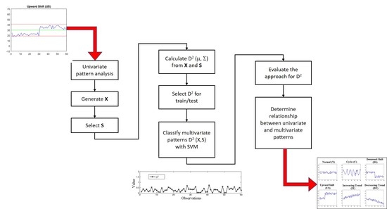
The purpose of this research is to recognise multivariate patterns in multivariate variables which is significant to SPC because the existence of an out-of-control condition locates the faults presented by the variables. The method proposes observation of multivariate patterns during the measurement of multivariate variables. When a pattern is identified, it is proposed to associate the multivariate pattern with the variations and their causes reflected in the univariate variables that formed that multivariate variable. A previous analysis on system or process behaviour must be carried out with regard for the establishment of relationships between multivariate patterns and underlying causes.

Considering the above, the method consists of the following steps:

• Generate different types of multivariate variables.
• Select a multivariate variable in control or close to normality (C).
• Determine $D^2$ between C and multivariate variables X.
• Evaluate if $D^2$ exhibits multivariate variation classes using SVM.
• Determine the combination of variation classes.
• Recognise each type of multivariate pattern in $D^2$.
• Determine the variable’s location and the causes that originated them.

The method considers the generation of multivariate variables using the “Synthetic Control Chart Time Series” public database which is composed by variation-class carrying vectors (special patterns and natural patterns). Following this methodology, it is expected to find out about the existence of an association between the multivariate patterns observed in the $D^2$ and the patterns present in the univariate variables that formed each $D^2$. Two approaches are proposed for the calculation of $D^2$ with the aim of obtaining quantitative measurements of similarity between observations of multivariate variables and the centroid of other multivariate variables. The methodology is depicted in Figure 2.

1.3. Database Generation of Multivariate Variables

The “Synthetic Control Chart Time Series” database employed for our experiments was generated using control charts generated by the process described in Alcock RJ & Manolopoulos in [7]. In the database, there are 100 pattern samples for each corresponding pattern type such as Increasing Trend (IT), Decreasing Trend (DT), Downward Shift (DS), Upward Shift (US), Cycle (Cy) and Normal (N). Thus, there are 600 samples corresponding to synthetically generated control charts.

The proposed method considers p-variables of a random process $\mathbf{X}=[X_1,X_2,\dots ,X_p]$ defined as a multivariate variable. In this form, $\mathbf{X}$ is defined as a multivariate variable formed by p univariate variables. In this paper, we present the approach with $p=2$ univariate variables so that the composition of each multivariate variable is $\mathbf{X}=[X_1,X_2]$.

Table 1. Types of multivariate variables generated with 2 variables in $\mathbf{X}=[X_1,X_2]$. Increasing Trend (IT), Decreasing Trend (DT), Downward Shift (DS), Upward Shift (US), Cycle (Cy) and Normal (N).

X	${\mathit{X}}_1$	${\mathit{X}}_2$
$X_1$	N	Cy
$X_2$	N	IT
$X_3$	N	DT
$X_4$	N	US
$X_5$	N	DS
$X_6$	N	N
$X_7$	Cy	Cy
$X_8$	Cy	IT
$X_9$	Cy	DT
$X_{10}$	Cy	US
$X_{11}$	Cy	DS
$X_{12}$	Cy	N
$X_{13}$	IT	Cy
$X_{14}$	IT	IT
$X_{15}$	IT	DT
$X_{16}$	IT	US
$X_{17}$	IT	DS
$X_{18}$	IT	N
$X_{19}$	DT	Cy
$X_{20}$	DT	IT
$X_{21}$	DT	DT
$X_{22}$	DT	US
$X_{23}$	DT	DS
$X_{24}$	DT	N
$X_{25}$	US	Cy
$X_{26}$	US	IT
$X_{27}$	US	DT
$X_{28}$	US	US
$X_{29}$	US	DS
$X_{30}$	US	N
$X_{31}$	DS	Cy
$X_{32}$	DS	IT
$X_{33}$	DS	DT
$X_{34}$	DS	US
$X_{35}$	DS	DS
$X_{36}$	DS	N

shows the configuration of these multivariate classes. To determine the quantity of multivariate variable types, the permutation formula applied is: $n^r=(6^2)=36$; where n = types of patterns to choose from and r = number of elements that forms the permutation. The procedure consisted in choosing 100 samples containing a type of pattern for $X_1$ and another 100 samples for $X_2$ and combining them to form a type of multivariate variable as shown in Figure 3. Based on the above, 10,000 multivariate variable samples were generated for each of the 36 classes of multivariate variables $\mathbf{X}$ shown in Table 1, making a total of 360,000 sample patterns as population study.

1.4. The Mahalanobis Distance Calculation ($D^2$)

The use of Mahalanobis distance $D^2$ is proposed to determine the existence and representation of multivariate patterns in different multivariate classes. $D^2$ allows us to analyse the behaviour of multivariate variables providing a similarity measurement between observations comparing their centroids. As exposed in Section 1.2, the method requires the calculation of $D^2$ from a variable with stable behaviour, which, in this bivariate case, is the pattern represented by ${\mathbf{X}}_{\mathbf{6}}$ that includes natural patterns in its elements $[X_1,X_2]$. ${\mathbf{X}}_{\mathbf{6}}$ is then labelled as $\mathbf{C}$ to pinpoint its stable behaviour. Then, $D^2$ is calculated from $\mathbf{X}$ and $\mathbf{C}$.

Calculation of the Mahalanobis Distance $D^2$ with Respect to $\mathbf{X}$ and $\mathbf{C}$.

$D^2$ is computed from Equation (1) as follows:

$$D^2(\mathbf{X},\mathbf{C})={(\mathbf{X}-\overline{\mathbf{C}})}^T{\mathbf{S}}_{\mathbf{C}}^{-\mathbf{1}}(\mathbf{X}-\overline{\mathbf{C}})$$

(1)

where $\overline{\mathbf{C}}$ and ${\mathbf{S}}_{\mathbf{C}}$ are the mean and covariance from $\mathbf{C}$, respectively.

As an example, consider ${\mathbf{X}}_{\mathbf{7}}$, which is constituted by two univariate variables with cyclic patterns ${\mathbf{X}}_{\mathbf{7}}=[X_1,X_2]=[Cy,Cy]$. The Mahalanobis distance is then calculated between the observations of the multivariate variable $\mathbf{X}({\mathbf{X}}_{\mathbf{7}})$ and $(\overline{\mathbf{C}},{\mathbf{S}}_{\mathbf{C}})$ of the multivariate variable $\mathbf{C}({\mathbf{X}}_{\mathbf{6}})$. These values $D^2$ are shown in Figure 4.

The next step is to calculate the Mahalanobis distance $D^2$ between $\mathbf{C}$ and ($\overline{\mathbf{C}},{\mathbf{S}}_{\mathbf{C}}$) from each of the 360,000 patterns previously generated. $D^2$ is determined by Equation (2)

$$D^2(\mathbf{C},\mathbf{X})={(\mathbf{C}-\overline{\mathbf{X}})}^T{\mathbf{S}}_{\mathbf{X}}^{-\mathbf{1}}(\mathbf{C}-\overline{\mathbf{X}})$$

(2)

where $\overline{\mathbf{X}}$ and ${\mathbf{S}}_{\mathbf{X}}$ are the mean and covariance calculated from the multivariate variable $\mathbf{X}$. Similarly, a multivariate variable $\mathbf{X}$ is generated with the composition ${\mathbf{X}}_{\mathbf{7}}$ = $[X_1,X_2]$ = [Cy, Cy]. For the variable $\mathbf{C}$, a multivariate variable generated with the composition $\mathbf{X}\mathbf{6}=[X_1,X_2]$ = [N, N] was selected. Figure 5 shows the Mahalanobis distance calculation between the observations of $\mathbf{C}$ and $(\overline{\mathbf{X}}$, ${\mathbf{S}}_{\mathbf{X}})$ of $\mathbf{X}$.

It is desirable to find a characteristic behaviour for each class of $D^2$ related to the multivariate variable class it forms. In this way, the behaviour of the process could be determined by the information given by the $D^2$ calculation. The generated $D^2$ patterns were examined in both approaches, and no distinctive forms of multivariate patterns were found in comparison with the basic patterns in “Synthetic Control Chart Time Series” that originated them. SVM was proposed in order to determine if the multivariate pattern was identifiable, which is explained in the Section 1.5.

1.5. Multivariate Pattern Recognition

The Support Vector Machine (SVM) is used for multivariate pattern recognition using $D^2$. The principle of SVM is to find a hyperplane that solves the problem of classifying a data set. The classification is produced by the separation of data belonging to different classes through a hyperplane and maximising the margin between classes in such a way that the data belonging to the same class is located on the same side of the hyperplane [20].

In the case of linear classification, we have a training group of size n composed of the data vector $x_i\in R^n,i=1,\dots ,l$ in two classes labeled $y\in {\{+1,-1\}}^l$. The classification function is expressed by the Equation (3)

$$f(x)={\Sigma }_{i=1}^l{w}_i{x}_i+b$$

(3)

where vector $w\in {\mathbb{R}}^n$ defines the hyperplane slope and the parameter $b\in {\mathbb{R}}^n$ determines the optimal hyperplane. By means of the decision function $y=sign(w·x+b)$, it is expected to correctly classify both training and test data. However, most real problems do not have a normal distribution that can not be linearly separable. Given this case, the data from the input space (belonging to two different classes) must be mapped to the characteristics space of a larger dimension in such a way that the data be linearly separable through a hyperplane and the margin between the classes is maximized, with the process then reversed to the original dimension.

The data transformation was obtained through a kernel function which allows data separation. To find the best solution regarding the separation by the hyperplane, the following optimisation is proposed:

$$\underset{w,b,\xi }{min}\frac{1}{2}{w}^{T}w+C_k{\Sigma }_{i=1}^l{\xi }_i$$

(4)

subject to

$$\begin{array}{c}\hfill y_i(w^T·x_i+b)\ge 1-{\xi }_i,\\ \hfill {\xi }_i\ge 0,i=1,\dots ,l\end{array}$$

(5)

${\xi }_i>0$ is the error margin between the point i and the separation limits. Parameter $C_k$ can be interpreted as a tuneable parameter, where a higher value $C_k$ corresponds to establishing a greater importance to the task of correctly classifying the training data. A lower $C_k$ value implies a hyperplane with greater flexibility that attempts to minimise the margin of error for each sample. For the tuning of parameters ($C_k,a$) in the training process, the Mesh Search and Validation strategies were proposed. $C_k=32$ and $a=0.17$ were used.

Different kernel functions were tested such as polynomial, Radial Basis Function (RBF), and, finally, the sigmoid as indicated in the

Table 2. Support Vector Machine (SVM) Kernel functions and parameters.

Kernel	Function	Parameter
Polynomial	$k(x_i,y_j)=a{(x_i,y_j+r)}^d$	$C_k=32;a=0.17;r=0;d=3$
RBF	$k(x_i,y_j)=exp(-a\parallel X_i-X_j{\parallel }^2)$	$C_k=32;a=0.17$
Sigmoid	$k(x_i,y_j)=tanh(a{x}_i^T{y}_j+r)$	$C_k=32;a=0.17;r=0$

.

Simulation results during experiments using Equations (1) and (2) showed that the best kernel function was the sigmoid $k(x_i,y_j)=tanh(a{x}_i^T{y}_j+r)$, where $a>0$ is a scale parameter of input data and r is a displacement parameter controlling the mapping threshold [21]. These results are presented in Section 2.

Although SVM was designed to deal with binary classification problems, there are strategies that allow extension to the multiclass problem. One way to solve this problem is to consider it a series of binary classification problems. For the present work, it was decided to use the “one against all” strategy, where K SVM classifiers are built to differentiate each class from the others. In such a way that the ith classifier is trained with patterns of class i and value 1, the rest of the patterns’ classes are trained with a value of $-1$.

Distances $D^2$ were calculated to integrate the training and the test base. The 360,000 $D^2$ were divided into 36 classes corresponding to the classes of the multivariate variables with which they were calculated, i.e., 10,000. The training and test bases were analysed with SVM. In the training stage, SVM used the training database and a labelled vector to learn and recognise each multivariate pattern corresponding to each $D^2$ class. The outputs produced in the training stage by the SVM can be interpreted as the correct or incorrect learning of each $D^2$.

For the test stage, the $D^2$ of the test base is analysed using SVM with an unknown input. It is expected the SVM to be able to recognise it through the knowledge acquired in the training stage. In the test stage, by effectively recognising the types of multivariate patterns in the $D^2$, it is possible to define the exact pattern $(\mathbf{C},\mathbf{X})$ the distances were obtained from (similar to the way Table 1 was obtained). In addition, the patterns in $X_1$ and $X_2$ that make up each of the multivariate variables $\mathbf{X}$ with which the distances were calculated can be known. Also, by knowing the patterns in $X_1$ and $X_2$ it can be defined whether these variables are in-control or out-of-control. Similarly, it is possible to relate and infer what type of pattern each vector of the multivariate variable contains and associate it with its type of failure according to the Western Electric Manual [8]. In Section 2, the experimental results are presented.

2. Experimental Results

With the training and testing data bases for SVM and the $D^2$, a set of three experiments were performed with different variables. The parameters shown in

Table 3. Experimental parameters for SVM and $D^2$.

	${\mathit{D}}^2$ Calculated from C	${\mathit{D}}^2$ Calculated from X
SVM $(C_k,a)$	$C_k=32;a=0.17$	$C_k=32$; $a=0.17$
	$\overline{\mathbf{C}}=\left[\begin{array}{cc}30.1183& 29.4810\end{array}\right]$
$D^2$ ($\overline{\mathbf{C}}$; ${\mathbf{S}}_{\mathbf{C}}$)	${\mathbf{S}}_{\mathbf{C}}^{-\mathbf{1}}=\left[\begin{array}{cc}0.0795& 0.0021\\ 0.0021& 0.0739\end{array}\right]$	$\overline{\mathbf{C}}$, ${\mathbf{S}}_{\mathbf{C}}^{-\mathbf{1}}$ are calculated for each $\mathbf{X}$
	Calculated from $\mathbf{C}$

were used in the experiments.

2.1. Multivariate Pattern Recognition in Mahalanobis Distances Calculated with Statistical of Multivariate Variable $\mathbf{C}$

This experiment was made with the intention of determining the efficiency of multivariate pattern recognition in the 360,000 $D^2$ values obtained with Equation (1).

Table 4. $D^2$ Recognition with SVM and $\mathbf{C}$.

Multivariate Pattern Recognition (C)
No	Training Set	Testing Set	Ratio (Training/Testing)	Recognition (%)
1	144	72	2	8.33
2	36,000	72,000	0.5	36.56
3	108,000	252,000	0.43	35.93

shows the results. As it can be observed, in the three cases, the recognition percentage is low despite the size of the testing set.

2.2. Multivariate Pattern Recognition in Mahalanobis Distances Calculated with Statistical of Multivariate Variable $\mathbf{X}$

In the same way as in the previous approach, three experiments were performed with different variables in the training and testing databases for the SVM. In this case, the 360,000 $D^2$ values were obtained using Equation (2).

Table 5. $D^2$ Recognition with SVM and $\mathbf{X}$.

Multivariate Pattern Recognition (X)
No	Training Set	Testing Set	Ratio (Training/Testing)	Recognition (%)
1	144	72	2	91.66
2	36,000	72,000	0.5	83.8
3	108,000	252,000	0.43	70.92

shows the results; the recognition percentage increased in these three experiments when calculating the $D^2$ with the proposed approach.

As it can be observed from Table 5, the recognition is higher with a high training/testing ratio as it was expected. The following step according to our approach would be to determine the corresponding $X_1$ and $X_2$ patterns that make up the multivariate variable. Consequently, by knowing the $X_1$ and $X_2$ patterns, one can define which control action to take according to the X pattern type.

3. Conclusions

In this paper, a method to recognise univariate patterns in multivariate patterns using the Mahalanobis distance has been shown. The method determines the association of multivariate patterns with univariate variables. During experiments, multivariate patterns formed by Mahalanobis distances were calculated with different multivariate variables. When visually inspecting the types of multivariate patterns as observed in the 36 classes of $D^2$, no distinctive forms were found for each type of multivariate pattern compared to the characteristic forms presented by the univariate patterns of the “Synthetic Control Chart Time Series”. This was our main motivation for interchangeably analysing $\mathbf{C}$, and $\mathbf{X}$ cases and their differences using the Mahalanobis distance through SVM recognition.

A first set of experiments (stable case with $\mathbf{C}$) was presented, the computing of distances $D^2$ and the rest of multivariate pattern recognition was made using SVM obtaining a recognition rate as low as $8.33\%$. A second set of experiments (unstable case) was envisioned and the outcome was far better than in the first experiment; in this second approach, a recognition of $91.67\%$ was obtained with a training/testing ratio of 2.

The relevance of this research lies upon the calculation of the $D^2$ between a multivariate variable (with natural patterns) and the statistical values ($\overline{C}$, $S_C$, $S_X$) of each of the generated multivariate variables. This modification saw an increase to the difference between each of the types or classes of multivariate patterns compared to other works that use Hotelling, MEWMA [22], PCA, combination of variables and scatter plot [23]. Our own results showed that using $T^2$ with the synthetic data base resulted in efficiencies as low as 27.99%.

An important observation is that our proposal considered the calculation of covariance matrices by sub-data sets since these were obtained directly from the application of Equation (2). For each equation the parameters $\overline{\mathbf{X}}$ and ${\mathbf{S}}_{\mathbf{X}}$ adjust to the changing values contained in the different combinations of X patterns and fixed periods were considered for the covariance matrix. However, an envisaged recognition of multivariate patterns using the periods of the covariance matrix in order to observe the changes in this matrix period by period would certainly reinforce our method.

By recognising each class or type of distance of Mahalanobis correctly, it is possible to make out the composition ($\mathbf{C},\mathbf{X}$) of each distance of Mahalanobis. In addition, there is the potential ability to infer the composition ($X_1$ and $X_2$) of each multivariate variable $\mathbf{X}$. Finally, by knowing the univariate patterns, it will be possible to infer errors that triggered them. If the number of variables increase, then the approach can also be used to find differentiable multivariate patterns for each type of classes, which is an ongoing research work.