Positive Solutions of the Fractional SDEs with Non-Lipschitz Diffusion Coefficient

Abstract

We study a class of fractional stochastic differential equations (FSDEs) with coefficients that may not satisfy the linear growth condition and non-Lipschitz diffusion coefficient. Using the Lamperti transform, we obtain conditions for positivity of solutions of such equations. We show that the trajectories of the fractional CKLS model with $\beta >1$ are not necessarily positive. We obtain the almost sure convergence rate of the backward Euler approximation scheme for solutions of the considered SDEs. We also obtain a strongly consistent and asymptotically normal estimator of the Hurst index $H>1/2$ for positive solutions of FSDEs.

1. Introduction

The models defined by stochastic differential equations (SDEs)

$$X_t=x_0+{\int }_0^{t}g\left(X_s\right)ds+ {\int }_0^t{X}_s^{\beta }d{B}_s,\hspace{1em}\hspace{1em}\beta ⩾1/2,\hspace{1em}\beta \ne 1,$$

(1)

where B is a standard Brownian motion, g is a continuous function on $(0,\infty )$, $x_0>0$ is nonrandom initial value, and $\sigma >0$ is a constant, include several well-known models such as Chan–Karolyi–Longstaff–Sanders (CKLS), Cox–Ingersoll–Ross (CIR), Ait–Sahalia (AS), Cox–Ingersoll–Ross variable-rate (CIR VR), and others used in many financial applications [1,2,3,4,5,6]. The positivity is a desirable property for many financial models, such as option pricing, stochastic volatility, and interest rate models. Thus, it is important to find conditions under which the solutions to Equation (1) are positive. Preservation of positivity is a desirable modelling property, and in many cases the non-negativity of numerical approximations is needed for the scheme to be well defined. Therefore, many numerical methods have been developed to preserve the positivity of the approximate solution in the case of the positive true solution.

For an SDE to have a unique global solution (i.e., with no explosion in a finite time) for any given initial value, the coefficients of the equation are in general required to satisfy the linear growth and local Lipschitz conditions. These conditions are not satisfied in the models mentioned. The existence of positive solutions of SDEs corresponding to these models and implicit numerical schemes preserving the positivity were studied in [1,2,3,4,5,6].

An important research area in financial mathematics is the long memory phenomenon in financial data. Hence, since fractional Brownian motion (fBm) $B^H$ introduces a memory element, there is much attention in recent years to models with fBm. Consider the FSDEs

$$X_t=x_0+{\int }_0^{t}g\left(X_s\right)ds+\sigma {\int }_0^t{X}_s^{\beta }d{B}_s^H,\hspace{1em}\hspace{1em}\beta ⩾1/2,\hspace{1em}\beta \ne 1,$$

(2)

with $H\in (1/2,1)$. The stochastic integral in Equation (2) is a pathwise Riemann–Stieltjes integral, but SDE (2) cannot be treated directly since the functions $k\left(x\right)=x^{\beta }$, $\beta ⩾1/2$, $\beta \ne 1$, do not satisfy the usual Lipschitz conditions.

For fractional CIR, CKLS, and AS models, the existence of a unique positive solution of Equation (2) was obtained in [7,8,9,10,11,12,13,14]. The proof can be provided in several ways. One approach is based on the consideration of the conditions under which the equation

$$Y_t=y_0+{\int }_0^{t}h(s,Y_s)ds+B_t^H,\hspace{1em}\hspace{1em}H\in (1/2,1),$$

(3)

admits a unique positive solution, where $h(t,x)$ is a locally Lipschitz function with respect to the space variable $x\in (0,\infty )$. This approach was used in [7,8,9,11,14], where the inverse Lamperti transform was used to obtain conditions under which Equation (1) admits a unique positive solution for fractional CIR, CKLS, and AS models. Unfortunately, we cannot apply the proof of positivity of the solution of (3) given in [14] (e.g., it is not applicable to the AS model).

Marie [10] used the rough-path approach to find the existence of a unique positive solution of the fractional CKLS model.

A simulation of the fractional CIR process was given in [11] by using the Euler approximation. In [8,14] an almost sure strongly convergent approximation of the considered SDE solution is constructed using the backward Euler scheme, which is positivity preserving.

In this paper, we consider the SDE

$$Y_t=y_0+(\beta -1){\int }_0^{t}h\left(Y_s\right)ds-(\beta -1)\sigma B_t^H,\hspace{1em}\hspace{1em}\beta >1,$$

(4)

where $y_0$ is a constant. This type of equation is obtained after the Lamperti transformation of the FSDE (2). The purpose of the paper is finding sufficiently simple conditions when the solution of (4) for $\beta >1$ and $H\in (1/2,1)$ is positive. Moreover, using the backward Euler scheme, which preserves the positivity for (4), we obtain an almost sure convergence rate for X. Since the problem of the statistical estimation of the long-memory parameter H is of great importance, we construct an estimate of the Hurst index $H\in (1/2,1)$ in the same way as for the diffusion coefficient satisfying the usual Lipschitz conditions (see [15,16]). This can be done since the solution of Equation (2) is positive. More results on parameter estimations for the FSDEs can be found in the book [17].

The paper is organized as follows. In Section 2, we present the main results of the paper. In Section 3, we prove the main auxiliary result on the existence and uniqueness of a positive solution for SDE (4). Section 4 contains proofs of the main theorems. In Section 5, we consider fractional CKLS and AS models as examples. Finally, in Appendix A, we recall the Love–Young inequality, the chain rule for Hölder-continuous functions, and some results for fBm.

2. Main Results

We are interested in conditions under which the SDE

$$X_t=x_0+{\int }_0^t{X}_s^{\beta }f\left(X_s^{1-\beta }\right)ds+\sigma {\int }_0^t{X}_s^{\beta }d{B}_s^H,\hspace{1em}\hspace{1em}\beta >1, H\in (1/2,1),$$

(5)

has a unique positive solution. The stochastic integral in Equation (5) is a pathwise Riemann–Stieltjes integral.

To state our main results, we assume that the following conditions on the function f in (5) are satisfied:

$\left({\mathbf{C}}_1\right)$f is a locally Lipschitz on $(0,+\infty )$;

$\left({\mathbf{C}}_2\right)$ There exist constants $a>0$ and $\alpha ⩾0$ such that

$$\widehat{f}\left(x\right):=-f\left(x\right)⩾\frac{a}{x^{1+\alpha }}$$

for all sufficiently small $x\in (0,\infty )$;

$\left({\mathbf{C}}_3\right)$ The function $\widehat{f}\left(x\right)$ satisfies the one-sided Lipschitz condition, that is, there exists a constant $K\in \mathbb{R}$ such that

$$(x-y)(\widehat{f}\left(x\right)-\widehat{f}\left(y\right))⩽K{(x-y)}^2$$

for all $x,y\in (0,+\infty )$.

Theorem 1. 

If a function f satisfies conditions $\left({\mathbf{C}}_1\right)$–$\left({\mathbf{C}}_3\right)$, then Equation (5) is well defined and has a unique positive solution $X\in {\mathcal{C}}^{\gamma }\left([0,T]\right)$ of order $\gamma \in (\frac{1}{2},H)$ for $H\in (\frac{1}{2},1)$, where ${\mathcal{C}}^{\gamma }\left([0,T]\right)$ denotes the space of Hölder-continuous functions of order $\gamma >0$ on $[0,T]$.

Consider the SDE

$$Y_t=y_0+(\beta -1){\int }_0^t\widehat{f}\left(Y_s\right)ds-(\beta -1)\sigma B_t^H,\hspace{1em}{y}_0=x_0^{1-\beta },\hspace{1em}\hspace{1em}t⩾0,\hspace{1em}H\in (\frac{1}{2},1).$$

(6)

A strong approximation of the SDE that has locally Lipschitz drift for $H\in (\frac{1}{2},1)$ is constructed by applying the backward Euler scheme in [14] (see also [1] for $H=\frac{1}{2}$). By using the backward Euler scheme, which preserves positivity for (6), we obtain an almost sure convergence rate for X.

A sequence of uniform partitions of the interval $[0,T]$ we denote by $\pi =\{t_k^n=\frac{k}{n}T,1⩽k⩽n\}$ and let and $h=t_k^n-t_{k-1}^n$, $1⩽k⩽n$. We introduce the backward Euler approximation scheme for Y

$$Y_{n,k+1}=Y_{n,k}+(\beta -1)\widehat{f}\left(Y_{n,k+1}\right)h-\sigma (\beta -1)\left(B_{t_{k+1}^n}^H-B_{t_k^n}^H\right),\hspace{1em}{Y}_{n,0}=y_0,\hspace{1em}0⩽k⩽n-1.$$

(7)

The following assumption is needed for the positivity of the backward Euler approximation scheme to be preserved:

$\left({\mathbf{C}}_4\right)$ Let $\widehat{F}\left(x\right)=x-(\beta -1)\widehat{f}\left(x\right)h$ on $(0,\infty )$, where the function $\widehat{f}\left(x\right)$ satisfies condition $\left({\mathbf{C}}_3\right)$. There exists $h_0>0$ such that ${\lim }_{x\to +\infty }\widehat{F}\left(x\right)=+\infty$ and ${\lim }_{x\to 0^{+}}\widehat{F}\left(x\right)=-\infty$ for $0<h<h_0$.

Remark 1. 

Please note that under condition $\left({\mathbf{C}}_3\right),$ the function $\widehat{F}\left(x\right)$ is strictly monotone on $(0,\infty )$ for small h. This follows from $\left({\mathbf{C}}_3\right)$ and the inequality

$$(x-y)(\widehat{F}\left(x\right)-\widehat{F}\left(y\right))={(x-y)}^2-(\beta -1)(x-y)(\widehat{f}\left(x\right)-\widehat{f}\left(y\right))h⩾(1-K^{+}(\beta -1)h){(x-y)}^2>0,$$

where $K^{+}=\max \{0,K\}$. Thus, from the condition $\left({\mathbf{C}}_4\right)$ it follows that for each $b\in \mathbb{R}$, the equation $F\left(x\right)=b$ has a unique positive solution for $0<h<h_0$. As a result, we see that the positivity is preserved by the backward Euler approximation scheme.

For the simplicity of notation, we introduce the symbol $O_{\omega }$. Let $\left(Z_n\right)$ be a sequence of r.v.s, let $\varsigma$ be an a.s. nonnegative r.v., and let $\left(a_n\right)\subset (0,\infty )$ be a vanishing sequence. Then $Z_n=O_{\omega }\left(a_n\right)$ means that $|Z_n|\le \varsigma ·a_n$ for all n. In particular, $Z_n=O_{\omega }\left(1\right)$ means that the sequence $\left(Z_n\right)$ is a.s. bounded.

Theorem 2. 

Suppose that the function f in (5) is continuously differentiable on $(0,+\infty )$ and satisfies condition $\left({\mathbf{C}}_2\right)$ and that there exists a constant $K\in \mathbb{R}$ such that the derivative is bounded above by K, that is, $f^{\prime }\left(x\right)⩽K$. If the sequence of uniform partitions π of the interval $[0,T]$ is such that $h<h_0$, then for all $T>0$ and $H\in (\frac{1}{2},1)$,

$$\underset{0⩽t⩽T}{\sup }|Y_t-Y_t^n|=O_{\omega }\left(n^{-H}\sqrt{\ln n}\right),$$

(8)

where

$$Y_t^n=Y_{n,k}+\frac{t-t_k^n}{h}\left(Y_{n,k+1}-Y_{n,k}\right),\hspace{1em}\hspace{1em}t\in (t_k^n,t_{k+1}^n], k=0,\dots ,n-1,\hspace{1em}{Y}_{n,0}^n=y_0.$$

Moreover,

$$\underset{0⩽t⩽T}{\sup }\left|X_t-{\left(Y_t^n\right)}^{-1/(\beta -1)}\right|=\left\{\begin{array}{cc}{O}_{\omega }\left(n^{-H}\sqrt{\ln n}\right)\hfill & for\beta \in (1,2],\hfill \\ O_{\omega }\left({\left(n^{-H}\sqrt{\ln n}\right)}^{1/(\beta -1)}\right)\hspace{1em}\hfill & for\beta >2,\hfill \end{array}\right.$$

(9)

where X is the solution of Equation (5).

For positive solutions of Equation (5), we construct a strongly consistent and asymptotically normal estimator of the Hurst parameter H from discrete observations of a single sample path.

For a real-valued process $X=\{X_t,t\in [0,T]\}$, we define the second order increments along uniform partitions as

$${\mathrm{\Delta }}_{n,k}^{\left(2\right)}X=X_{t_{k+1}^n}-2X_{t_k^n}+X_{t_{k-1}^n},\hspace{1em}1⩽k⩽n-1.$$

Theorem 3. 

Let X be a unique positive solution of SDE (5) with $H\in (\frac{1}{2},1)$. Then

$${\widehat{H}}_n=H+O_{\omega }\left({\left(\frac{\ln n}{n}\right)}^{1/2}\right)$$

and

$$2\ln 2\sqrt{n}({\widehat{H}}_n-H)\stackrel{d}{\to }\mathcal{N}(0,{\sigma }_H^2)$$

with known variance ${\sigma }_H^2$ defined in Appendix, where

$${\widehat{H}}_n=\frac{1}{2}-\frac{1}{2\ln 2}\ln \left(\frac{{\tilde{V}}_{2n,T}^{\left(2\right)X}}{{\tilde{V}}_{n,T}^{\left(2\right)X}}\right),\hspace{1em}\hspace{1em}{\tilde{V}}_{n,T}^{\left(2\right)X}={\displaystyle \sum _{k=1}^{n-1}}{\left(\frac{{\mathrm{\Delta }}_{n,k}^{\left(2\right)}X}{X_{t_k^n}^{\beta }}\right)}^2.$$

3. Auxiliary Results

As mentioned in Introduction, we are interested in conditions under which the SDE (6) has a unique positive solution.

Proposition 1. 

Suppose that a function f satisfies conditions $\left({\mathbf{C}}_1\right)$–$\left({\mathbf{C}}_3\right)$. If $y_0>0$, $k_1>0$, and $k_2\in \mathbb{R}$, then there exists a unique positive solution of Equation (6) such that $Y\in {\mathcal{C}}^{\gamma }\left([0,T]\right)$, $T>0$, where $\gamma \in (\frac{1}{2},H)$ and $H\in (\frac{1}{2},1)$.

We easily to see that the same proof as in Proposition 1 [8] remains valid for Proposition 1.

Applying Proposition 1 to the fractional AS model and Heston-3/2 volatility model, we obtain that the trajectories of these models are positive (see Section 5). Our proof scheme gives no answer about the behavior of the trajectories of the CKLS model

$$X_t=x_0+{\int }_0^t(a_1-a_2{X}_s)ds+\sigma {\int }_0^t{X}_s^{\beta }d{B}_s^H,\hspace{1em}\hspace{1em}\beta >1,\hspace{1em}H\in (\frac{1}{2},1),$$

(10)

with the initial value $x_0>0$ and deterministic constants $a_1>0$, $a_2\in \mathbb{R}$, and $\sigma >0$.

Now we will explain why we cannot give an answer about the behavior of the trajectories of the CKLS model. Consider the SDE

$$Y_t=y_0+(\beta -1){\int }_0^t(a_2{Y}_s-a_1{Y}_s^{\beta /(\beta -1)})ds-(\beta -1)\sigma B_t^H,\hspace{1em}\hspace{1em}H\in (\frac{1}{2},1).$$

(11)

Suppose that the solution of the SDE (11) is positive. Then by applying the chain rule (see Appendix A.2) and the inverse Lamperti transform $X_t=Y_t^{-1/(\beta -1)}$ we can prove that X is a positive solution of (10).

Unfortunately, it is easy to see that the function $\widehat{f}\left(x\right)=a_{2}x-a_1{x}^{\beta /(\beta -1)}$ does not satisfy condition $\left({\mathbf{C}}_2\right)$. So, we cannot apply Proposition 1 and say anything about the positivity of the solution of (11).

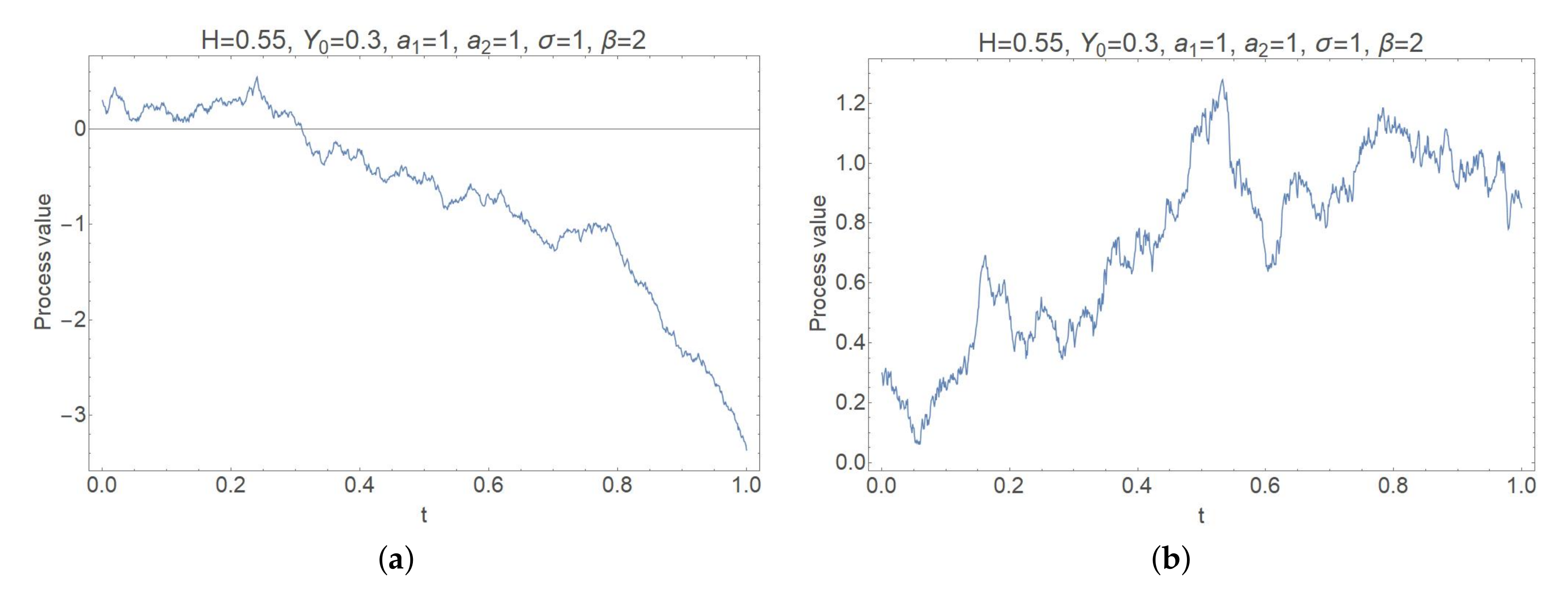
Computer modelling using Wolfram Mathematica shows that the trajectories of the process Y may have negative values for $y_0>0$ (see Figure 1).

Figure 1. Trajectory of Y: (a) with negative values. (b) with positive values.

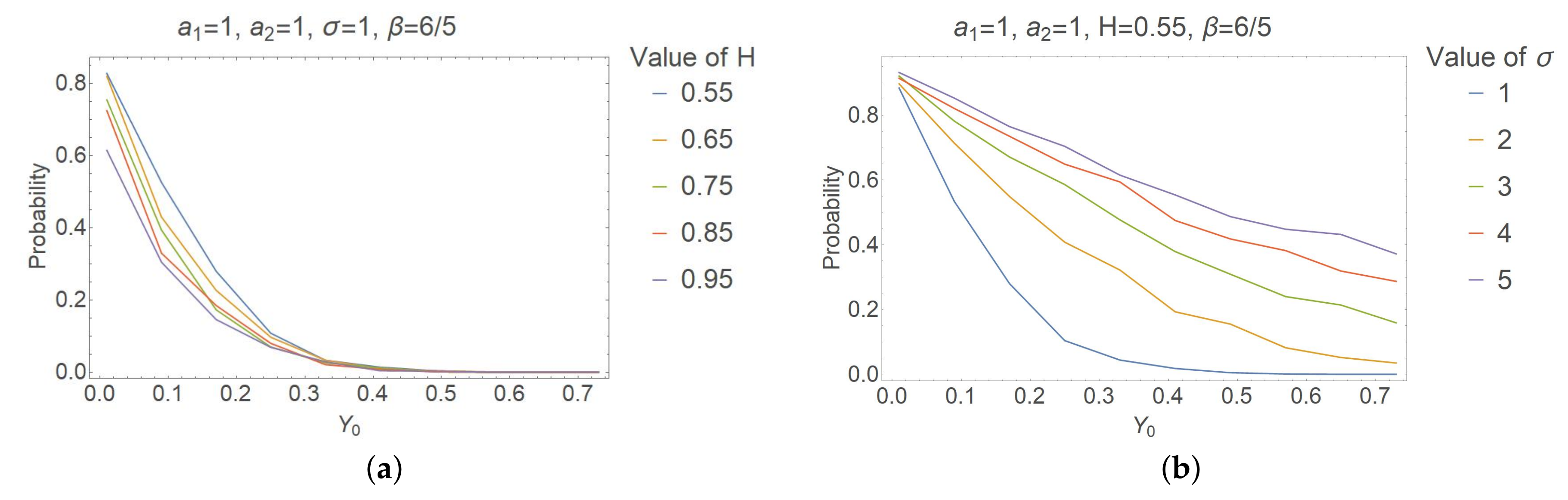
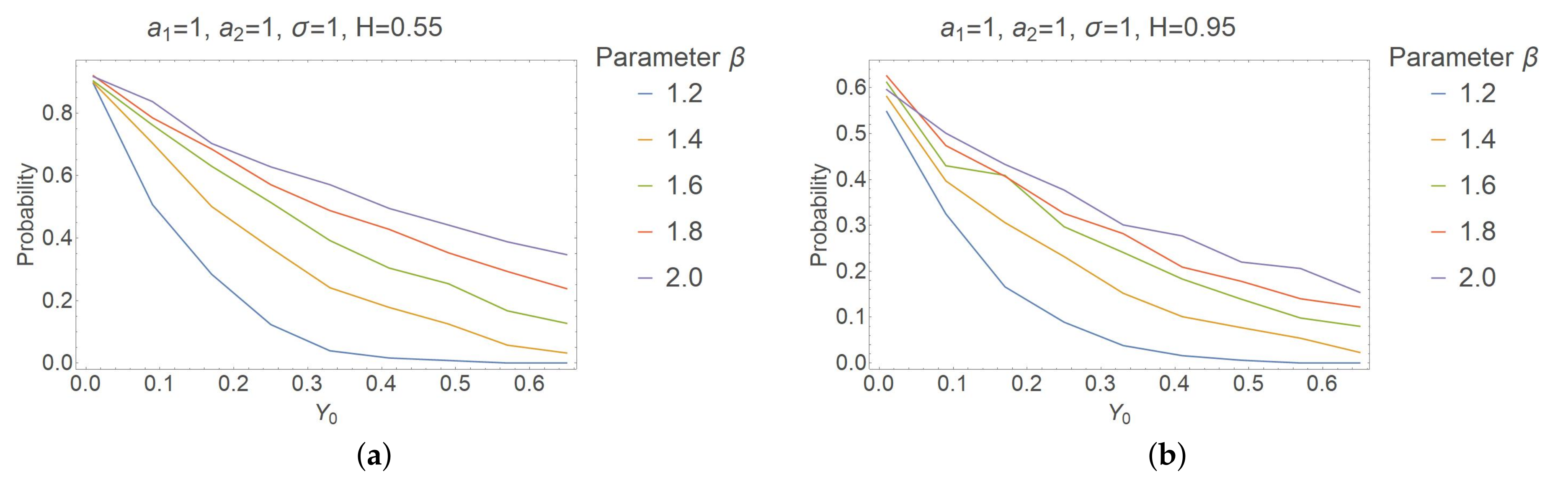
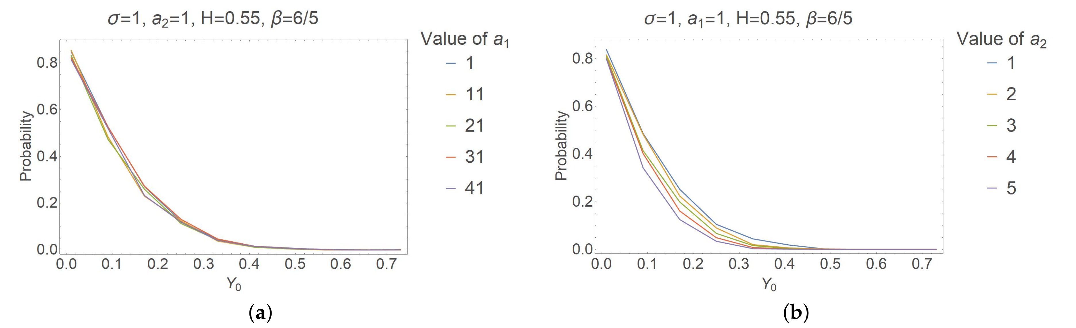
To investigate the probability of reaching the negative values by the process Y when $t\in [0,1]$, we simulate the “exact” solution by using the backward Euler approximation scheme for step size $h={10}^{-3}$ and repeat this process ${10}^3$ times counting the trajectories with negative values. We observe that the solution has a higher probability to reach the negative values for small initial values $Y_0$ and that for large enough values of $Y_0$, this probability tends to zero. Additionally, the probability increases for greater values of the parameters $\sigma ,\beta$ (see Figure 2b and Figure 3) and decreases for greater values of the parameters $H,a_2$ (see Figure 2a and Figure 4b). The influence of $a_1$ on the probability (see Figure 4a) is not noticeable in comparison with other parameters.

Figure 2. Probability that the trajectories have negative values: (a) Dependence of probability on $Y_0$ for different H. (b) Dependence of probability on $Y_0$ for different $\sigma$.

Figure 3. Probability that the trajectories have negative values: (a) Dependence of probability on $\beta$ when $H=0.55$. (b) Dependence of probability on $\beta$ when $H=0.95$.

Figure 4. Probability that the trajectories have negative values: (a) Dependence of probability on $a_1$. (b) Dependence of probability on $a_2$.

Thus, we can only state that Equation (10) has a solution $X_t=Y_t^{-1/(\beta -1)}$ until the moment at which Y becomes zero. On the other hand, we do know that the CKLS model driven by a standard Brownian motion (see [6]) with $\beta >1$ and the fractional CKLS model with $1/2⩽\beta <1$ (see [8]) have positive solutions.

4. Proofs

The main tool for proving Theorem 1 is Proposition 1.

Proof of Theorem 1. 

Set $X_t=Y_t^{-1/(\beta -1)}$ and $x_0=y_0^{-1/(\beta -1)}$, where Y is a solution of Equation (6). Since the process Y is positive and continuous, for $s,t\in [0,T]$, we get

$$\begin{array}{cc}\hfill |Y_t^{-\beta /(\beta -1)}-Y_s^{-\beta /(\beta -1)}|& =\frac{|Y_t^{\beta /(\beta -1)}-Y_s^{\beta /(\beta -1)}|}{Y_t^{\beta /(\beta -1)}{Y}_s^{\beta /(\beta -1)}}\hfill \\ & ⩽\frac{1}{{\inf }_{0⩽t⩽T}{Y}_t^{2\beta /(\beta -1)}}\frac{\beta }{\beta -1}\underset{0⩽t⩽T}{\sup }{Y}_t^{1/(\beta -1)}·\left|Y_t-Y_s\right|.\hfill \end{array}$$

(12)

Thus, $X_s^{\beta }$ is a Hölder-continuous process up to the order $\gamma \in (\frac{1}{2},H)$ on $[0,T]$. The process $X_t=Y_t^{-1/(\beta -1)}$ is the solution of Equation (5). Indeed, by chain rule we obtain

$$\begin{array}{cc}\hfill X_t& =Y_t^{-1/(\beta -1)}=Y_0^{-1/(\beta -1)}-\frac{1}{\beta -1}{\int }_0^t{Y}_s^{-\beta /(\beta -1)}d{Y}_s\hfill \\ & =y_0^{-1/(\beta -1)}-\frac{\beta -1}{\beta -1}{\int }_0^t{Y}_s^{-\beta /(\beta -1)}\widehat{f}\left(Y_s\right)ds+\frac{\sigma (\beta -1)}{\beta -1}{\int }_0^t{Y}_s^{-\beta /(\beta -1)}d{B}_s^H\hfill \\ & =x_0+{\int }_0^{t}g\left(X_s\right)ds+\sigma {\int }_0^t{X}_s^{\beta }d{B}_s^H.\hfill \end{array}$$

□

Proof of Theorem 2. 

We repeat the outlines of the proof of Theorem 3 in [8]. Please note that under the conditions of the theorem, conditions $\left({\mathbf{C}}_1\right)$–$\left({\mathbf{C}}_3\right)$ are satisfied. Thus, there exists a unique positive solution of SDE (6).

By the definition of $Y^n$, for any $t\in (t_k^n,t_{k+1}^n]$, we have

$$\begin{array}{cc}\hfill Y_t-Y_t^n=& Y_t-\frac{t-t_k^n}{h}{Y}_{n,k+1}-\frac{t_{k+1}^n-t}{h}{Y}_{n,k}\hfill \\ \hfill =& \frac{t_k^n-t}{h}(\beta -1)\left[{\int }_t^{t_{k+1}^n}\widehat{f}\left(Y_s\right)ds-\sigma \left(B_{t_{k+1}^n}^H-B_t^H\right)\right]\hfill \\ \hfill \hspace{1em}& +\frac{t_{k+1}^n-t}{h}(\beta -1)\left[{\int }_{t_k^n}^t\widehat{f}\left(Y_s\right)ds-\sigma \left(B_t^H-B_{t_k^n}^H\right)\right]\hfill \\ \hfill \hspace{1em}& +\frac{t-t_k^n}{h}\left(Y_{t_{k+1}^n}-Y_{n,k+1}\right)+\frac{t_{k+1}^n-t}{h}\left(Y_{t_k^n}-Y_k\right).\hfill \end{array}$$

Since the process Y is positive and continuous, from (A5) it follows that

$$\begin{array}{cc}\hfill |Y_t-Y_s|& ⩽(\beta -1){\int }_s^t\left|\widehat{f}\left(Y_u\right)\right|du+(\beta -1)\sigma |B_t^H-B_s^H|\hfill \\ & ⩽(\beta -1)(t-s)\underset{0⩽u⩽T}{\sup }|\widehat{f}\left(Y_u\right)|+(\beta -1)K_{\omega }{\left|t-s\right|}^H\sqrt{\left|\ln \left|t-s\right|\right|}\hfill \\ & =O_{\omega }\left({\left|t-s\right|}^H\sqrt{\left|\ln \left|t-s\right|\right|}\right),\hfill \end{array}$$

and the asymptotic behavior of the first two terms is $O_{\omega }\left(n^{-H}\sqrt{\ln n}\right)$. Thus, it remains to obtain the asymptotics of the last two terms.

Please note that

$$\begin{array}{cc}\hfill Y_{t_{k+1}^n}-Y_{n,k+1}=& Y_{t_k^n}-Y_{n,k}+(\beta -1){\int }_{t_k^n}^{t_{k+1}^n}\left[\widehat{f}\left(Y_s\right)-\widehat{f}\left(Y_{n,k+1}\right)\right]ds\hfill \\ \hfill \hspace{1em}& +(\beta -1)\sigma {\zeta }_{k+1}(Y_{t_{k+1}^n}-Y_{n,k+1})h,\hfill \end{array}$$

where ${\zeta }_{k+1}={\widehat{f}}^{\prime }(Y_{t_{k+1}^n}+\theta (Y_{n,k+1}-Y_{t_{k+1}^n}))$, $\theta \in (0,1)$. Then

$$\begin{array}{cc}\hfill Y_{t_{k+1}^n}-Y_{n,k+1}=& \frac{1}{1-(\beta -1){\zeta }_{k+1}h}\left[Y_{t_k^n}-Y_{n,k}+(\beta -1){\int }_{t_k^n}^{t_{k+1}^n}\left[\widehat{f}\left(Y_s\right)-\widehat{f}(Y_{t_{k+1}^n})\right]ds\right]\hfill \\ \hfill =& {\displaystyle \sum _{i=1}^{k+1}}{I}_i{\displaystyle \prod _{j=i}^{k+1}}{\left(1-{\zeta }_j(\beta -1)h\right)}^{-1},\hfill \end{array}$$

(13)

where

$$I_i=(\beta -1){\int }_{t_{i-1}^n}^{t_i^n}\left[\widehat{f}(Y_s)-\widehat{f}\left(Y_{t_i^n}\right)\right]ds.$$

Please note that $1-{\zeta }_i(\beta -1)h⩾1-(\beta -1)K^{+}h>0$ for $h<{\left((\beta -1)K^{+}\right)}^{-1}$ since $f^{\prime }\left(x\right)⩽K$, where $K^{+}=\max \{0,K\}$. Applying the inequality $\ln \frac{1}{1-x}⩽\frac{x}{1-x}$, $x<1$, we get

$$\begin{array}{cc}\hfill \prod _{j=i}^{k+1}{\left(1-{\zeta }_j(\beta -1)h\right)}^{-1}& {⩽(1-(\beta -1)K^{+}h)}^{-(k+1-i)}⩽e^{n\ln \frac{1}{1-(\beta -1)K^{+}h}}\hfill \\ & ⩽e^{n\frac{(\beta -1)K^{+}h}{1-(\beta -1)K^{+}h}}⩽e^{\frac{(\beta -1)K^{+}T}{1-(\beta -1)K^{+}h}}.\hfill \end{array}$$

Furthermore,

$$\left|{\int }_{t_{k-1}^n}^{t_k^n}\left[\widehat{f}\left(Y_s\right)-\widehat{f}\left(Y_{t_k^n}\right)\right]ds\right|⩽T{n}^{-1}\underset{0⩽t⩽T}{\max }|{\widehat{f}}^{\prime }\left(Y_t\right)|\underset{t_{k-1}^n⩽t⩽t_k^n}{\max }|Y_t-Y_{t_k^n}|=O_{\omega }\left(n^H\sqrt{\ln n}\right).$$

This finishes the proof of (8).

It remains to prove (9). We will use the well-known inequalities

$$\begin{array}{c}|x^p-y^p{|⩽|x-y|}^p,\hspace{1em}\hspace{1em}0<p<1,\hfill \\ |x^p-y^p{|<p|x-y\left|\right(\max \left\{\right|x|,|y\left|\right\})}^{p-1},\hspace{1em}\hspace{1em}p>1.\hfill \end{array}$$

Since $X_t=Y_t^{-1/(\beta -1)}$, we have

$${\sup }_{0⩽t⩽T}|X_t-{\left(Y_t^n\right)}^{-1/(\beta -1)}|={\sup }_{0⩽t⩽T}|Y_t^{-1/(\beta -1)}-{\left(Y_t^n\right)}^{-1/(\beta -1)}|={\sup }_{0⩽t⩽T}\frac{|Y_t^{1/(\beta -1)}-{\left(Y_t^n\right)}^{1/(\beta -1)}|}{Y_t^{1/(\beta -1)}{\left(Y_t^n\right)}^{1/(\beta -1)}}.$$

Please note that

$$\begin{array}{c}\hfill \underset{0⩽t⩽T}{\inf }{Y}_t^n⩾\underset{0⩽⩽n}{min}{Y}_{n,k}>0.\end{array}$$

Thus

$${\sup }_{0⩽t⩽T}|X_t-{\left({\widehat{Y}}_t^n\right)}^{-1/(\beta -1)}|⩽\left\{\begin{array}{cc}{\sup }_{0⩽t⩽T}\frac{|Y_t-\left({\widehat{Y}}_t^n\right){|}^{1/(\beta -1)}}{Y_t^{1/(\beta -1)}{\left({\widehat{Y}}_t^n\right)}^{1/(\beta -1)}}\hfill & \mathrm{if}\beta >2,\hfill \\ {\sup }_{0⩽t⩽T}\frac{|Y_t-{\widehat{Y}}_t^n|}{Y_t{\widehat{Y}}_t^n}\hfill & \mathrm{if}\beta =2,\hfill \\ \frac{1}{\beta -1}{\sup }_{0⩽t⩽T}\frac{|Y_t-{\widehat{Y}}_t^n|}{Y_t^{1/(\beta -1)}{\left({\widehat{Y}}_t^n\right)}^{1/(\beta -1)}}\hfill & \\ \times {\left(\max \left\{{\sup }_{0⩽t⩽T}|Y_t|,{\sup }_{0⩽t⩽T}\left|{\widehat{Y}}_t^n\right|\right\}\right)}^{\frac{2-\beta }{\beta -1}}\hspace{1em}\hfill & \mathrm{if}1<\beta <2.\hfill \end{array}\right.$$

From (8) and the finiteness of ${\sup }_{0\le t\le T}\left|Y_t\right|$ we have

$$\underset{0\le t\le T}{\sup }|{\widehat{Y}}_t^n|\le \underset{0\le t\le T}{\sup }|{\widehat{Y}}_t^n-Y_t|+\underset{0\le t\le T}{\sup }|Y_t|\le O_{\omega }\left(n^{-H}\sqrt{\ln n}\right)+\underset{0\le t\le T}{\sup }|Y_t|=O_{\omega }\left(1\right).$$

This finishes the proof of (9). □

Proof of Theorem 3.

Repeats the proof of Theorem 2 in [8]. It is based on the following lemma. □

Lemma 1. 

Assume that the conditions of Theorem 1 are satisfied and $\beta >1$. Then

$${\mathrm{\Delta }}_{n,i}^{\left(2\right)}X=\sigma X^{\beta }\left(t_i^n\right){\mathrm{\Delta }}_{n,i}^{\left(2\right)}{B}^H+O_{\omega }\left(n^{-2\gamma }\right),$$

where $\gamma \in (1/2,H)$.

Proof. 

Let $g\left(x\right)=x^{\beta }f\left(x^{1-\beta }\right)$. Then can we write the second-order increments of the process X as follows:

$$\begin{array}{cc}\hfill {\mathrm{\Delta }}_{n,k}^{\left(2\right)}X=& \left({\int }_{t_k^n}^{t_{k+1}^n}\left[g\left(X_s\right)-g\left(X_{t_k^n}\right)\right]ds-{\int }_{t_{k-1}^n}^{t_k^n}\left[g\left(X_s\right)-g\left(X_{t_k^n}\right)\right]ds\right)\hfill \\ & +\sigma \left({\int }_{t_k^n}^{t_{k+1}^n}\left[X_s^{\beta }-X_{t_k^n}^{\beta }\right]d{B}_s^H-{\int }_{t_{k-1}^n}^{t_k^n}\left[X_s^{\beta }-X_{t_k^n}^{\beta }\right]d{B}_s^H\right)\hfill \\ & +\sigma X_{t_k^n}^{\beta }{\mathrm{\Delta }}_{n,i}^{\left(2\right)}{B}^H.\hfill \end{array}$$

Applying inequality (12), condition $\left({\mathbf{C}}_1\right)$, and the fact that $Y\in {\mathcal{C}}^{\gamma }\left([0,T]\right)$, $\gamma \in (\frac{1}{2},H)$, we obtain

$$\begin{array}{cc}\hfill |g\left(X_t\right)-g\left(X_s\right)|& =|Y_t^{-\beta /(\beta -1)}f\left(Y_t\right)-Y_s^{-\beta /(\beta -1)}f\left(Y_s\right)|\hfill \\ & ⩽|f\left(Y_t\right)|·|Y_t^{-\beta /(\beta -1)}-Y_s^{-\beta /(\beta -1)}|+Y_s^{-\beta /(\beta -1)}\left|f\left(Y_t\right)-f\left(Y_s\right)\right|\hfill \\ & ⩽\underset{0⩽t⩽T}{\sup }|f\left(Y_t\right)|·\frac{1}{{\inf }_{0⩽t⩽T}{Y}_t^{2\beta /(\beta -1)}}\frac{\beta }{\beta -1}\underset{0⩽t⩽T}{\sup }{Y}_t^{1/(\beta -1)}·\left|Y_t-Y_s\right|\hfill \\ & \hspace{1em}+\underset{0⩽t⩽T}{\sup }{Y}_t^{-\beta /(\beta -1)}\underset{0⩽t⩽T}{\sup }|f^{\prime }\left(Y_t\right)|·|Y_t-Y_s|=O_{\omega }\left(n^{-\gamma }\right).\hfill \end{array}$$

Thus

$${\int }_{t_k^n}^{t_{k+1}^n}|g\left(X_s\right)-g\left(X_{t_k^n}\right)|ds=O_{\omega }\left(n^{-1-\gamma }\right)\hspace{1em}\mathrm{and}\hspace{1em}{\int }_{t_{i-1}^n}^{t_i^n}|g\left(X_s\right)-g\left(X_{t_k^n}\right)|ds=O_{\omega }\left(n^{-1-\gamma }\right).$$

Moreover, by the Love–Young inequality (see Appendix A.1), (12), and the Hölder continuity of $B^H$ we get

$$\left|{\int }_{t_{i-1}^n}^{t_i^n}\left[X_s^{\beta }-X_{t_i^n}^{\beta }\right]B_s^H\right|⩽C_{\gamma ,\gamma }\frac{1}{{\inf }_{0⩽t⩽T}{Y}_t^{2\beta /(\beta -1)}}\frac{\beta }{\beta -1}\underset{0⩽t⩽T}{\sup }{Y}_t^{1/(\beta -1)}{K}_{Y,T}{G}_{\gamma ,T}{n}^{-2\gamma },$$

where $K_{Y,T}={\sup }_{\begin{array}{c}s,t\in [0,T]\\ s\ne t\end{array}}\frac{|Y_t-Y_s|}{{\left|s-t\right|}^{\gamma }}<\infty$ a.s. Thus, the lemma is proved. □

5. Examples

Example 1. 

Ait–Sahalia model. The Ait–Sahalia-type SDE has the form

$$X_t=x_0+{\int }_0^t(a_1{X}_s^{-1}-a_2+a_3{X}_s-a_4{X}_s^r)ds+\sigma {\int }_0^t{X}_s^{\beta }d{B}_s^H$$

(14)

with the initial value $x_0>0$ and $r>2\beta -1$, where $H\in (\frac{1}{2},1)$, $\beta >1$, and deterministic constants $a_1,a_2,a_3,a_4>0$ and $\sigma >0$.

By using the Lamperti transformation $Y_t=X_t^{-(\beta -1)}$ we get

$$Y_t=y_0-(\beta -1){\int }_0^{t}f\left(Y_s\right)ds-\sigma (\beta -1)B_t^H=y_0+(\beta -1){\int }_0^t\widehat{f}\left(Y_s\right)ds-(\beta -1)\sigma B_t^H,$$

where $\widehat{f}\left(x\right)=-f\left(x\right)$ and

$$f\left(x\right)=a_1{x}^{\frac{\beta +1}{\beta -1}}-a_2{x}^{\frac{\beta }{\beta -1}}+a_{3}x-a_4{x}^{-\frac{r-\beta }{\beta -1}}.$$

The function f is continuously differentiable on $(0,+\infty )$. Condition $\left({\mathbf{C}}_2\right)$ is satisfied since

$$\widehat{f}\left(x\right)-\frac{a_4}{2}{x}^{-\frac{r-\beta }{\beta -1}}=\frac{a_4}{2}{x}^{-\frac{r-\beta }{\beta -1}}-a_1{x}^{\frac{\beta +1}{\beta -1}}+a_2{x}^{\frac{\beta }{\beta -1}}-a_{3}x\to \infty \hspace{1em}asx\to +0$$

with $a=a_4/2$, $\alpha =\frac{r-\beta }{\beta -1}-1>0$.

Now we verify condition $\left({\mathbf{C}}_3\right)$. Please note that

$$\begin{array}{cc}\hfill {\widehat{f}}^{\prime }\left(x\right)=& -a_1\frac{\beta +1}{\beta -1}{x}^{\frac{2}{\beta -1}}+a_2\frac{\beta }{\beta -1}{x}^{\frac{1}{\beta -1}}-a_3-a_4\frac{r-\beta }{\beta -1}{x}^{-\frac{r-1}{\beta -1}}\hfill \\ \hfill =& -x^{-\frac{r-1}{\beta -1}}\left(a_4\frac{r-\beta }{\beta -1}+a_1\frac{\beta +1}{\beta -1}{x}^{\frac{1+r}{\beta -1}}-a_2\frac{\beta }{\beta -1}{x}^{\frac{r}{\beta -1}}\right)-a_3\hfill \\ \hfill =& -x^{\frac{2}{\beta -1}}\left(a_1\frac{\beta +1}{\beta -1}-a_2\frac{\beta }{\beta -1}{x}^{-\frac{1}{\beta -1}}+a_4\frac{r-\beta }{\beta -1}{x}^{-\frac{r+1}{\beta -1}}\right)-a_3.\hfill \end{array}$$

Since the derivative $\widehat{f^{\prime }}\left(x\right)$ is continuous on $(0,\infty )$, ${\lim }_{x\to 0^{+}}\widehat{f^{\prime }}\left(x\right)=-\infty$, and ${\lim }_{x\to +\infty }\widehat{f^{\prime }}\left(x\right)=-\infty$, there is a constant K such that $\widehat{f^{\prime }}\left(x\right)⩽K$ for all $x\in (0,\infty )$.

Now the mean value theorem implies

$$(x-y)\left(\widehat{f}\left(x\right)-\widehat{f}\left(x\right)\right)={\widehat{f}}^{\prime }\left(c\right){(x-y)}^2⩽K{(x-y)}^2,$$

(15)

where $c=x+\theta (y-x)$, $\theta \in (0,1)$. Thus, Equation (14) has a unique positive solution on $(0,+\infty )$.

Let us verify condition $\left({\mathbf{C}}_4\right)$. Please note that

$$\begin{array}{cc}\hfill \widehat{F}\left(x\right)& =x-(\beta -1)\widehat{f}\left(x\right)h=x-(\beta -1)\left(-a_1{x}^{\frac{\beta +1}{\beta -1}}+a_2{x}^{\frac{\beta }{\beta -1}}-a_{3}x+a_4{x}^{-\frac{r-\beta }{\beta -1}}\right)h\hfill \\ & =(\beta -1)\left(a_1{x}^{\frac{\beta +1}{\beta -1}}-a_2{x}^{\frac{\beta }{\beta -1}}-a_4{x}^{-\frac{r-\beta }{\beta -1}}\right)h+\left(1+a_3(\beta -1)h\right)x\hfill \end{array}$$

is continuous on $(0,\infty )$. It is clear that $1+a_3(\beta -1)h>0$ for any $h>0$ and

$$\underset{x\to 0^{+}}{\lim }\widehat{F}\left(x\right)=-\infty \hspace{1em}and\hspace{1em}\underset{x\to +\infty }{\lim }\widehat{F}\left(x\right)=+\infty .$$

Since the function $\widehat{f}$ satisfies condition $\left({\mathbf{C}}_3\right)$, condition $\left({\mathbf{C}}_4\right)$ is satisfied as well. Therefore, the conditions of Theorem 2 are satisfied.

Example 2. 

Heston-3/2 volatility mode. Consider the SDE

$$X_t=x_0+{\int }_0^t{a}_1{X}_s(a_2-X_s)ds+\sigma {\int }_0^t{X}_s^{\beta }d{B}_s^H$$

(16)

with the initial value $x_0>0$, where $H\in (\frac{1}{2},1)$, $1<\beta <2$, and deterministic constants $a_1,a_2,\sigma >0$. If $\beta =3/2$, then we call the SDE (16) the fractional Heston-$3/2$ volatility model.

By using the Lamperti transformation $Y_t=X_t^{-(\beta -1)}$ we get

$$Y_t=y_0-(\beta -1){\int }_0^{t}f\left(Y_s\right)ds-\sigma (\beta -1)B_t^H=y_0+(\beta -1){\int }_0^t\widehat{f}\left(Y_s\right)ds-\sigma (\beta -1)B_t^H,$$

where $\widehat{f}\left(x\right)=-f\left(x\right)$ and

$$f\left(x\right)=a_1{a}_{2}x-a_1{x}^{-\frac{2-\beta }{\beta -1}}.$$

The function f is continuously differentiable on $(0,+\infty )$. Condition $\left({\mathbf{C}}_2\right)$ is satisfied since

$$\widehat{f}\left(x\right)-\frac{a_1}{2}{x}^{-\frac{2-\beta }{\beta -1}}=\frac{a_1}{2}{x}^{-\frac{2-\beta }{\beta -1}}-a_1{a}_{2}x\to \infty asx\to +0$$

with $a=a_1/2$, $\alpha =\frac{2-\beta }{\beta -1}-1>0$. Now we verify condition $\left({\mathbf{C}}_3\right)$. Please note that

$${\widehat{f}}^{\prime }\left(x\right)=-a_1{a}_2-a_1\frac{2-\beta }{\beta -1}{x}^{-\frac{1}{\beta -1}}<-a_1{a}_2.$$

Applying inequality (15), we obtain condition $\left({\mathbf{C}}_3\right)$. Thus, Equation (16) has a unique positive solution on $(0,+\infty )$. From the obtained result it follows that the Heston-$3/2$ volatility model has a unique positive solution on $(0,+\infty )$.

Let us verify condition $\left({\mathbf{C}}_4\right)$. Please note that

$$\begin{array}{cc}\hfill \widehat{F}\left(x\right)=& x-(\beta -1)\widehat{f}\left(x\right)h=x-(\beta -1)\left(-a_1{a}_{2}x+a_1{x}^{-\frac{2-\beta }{\beta -1}}\right)h\hfill \\ & =\left(1+a_1{a}_2(\beta -1)h\right)x-(\beta -1)a_1{x}^{-\frac{2-\beta }{\beta -1}}h\hfill \end{array}$$

is continuous on $(0,\infty )$. It is clear that $1+a_3(\beta -1)h>0$ for any $h>0$ and

$$\underset{x\to 0^{+}}{\lim }\widehat{F}\left(x\right)=-\infty \hspace{1em}and\hspace{1em}\underset{x\to +\infty }{\lim }\widehat{F}\left(x\right)=+\infty .$$

Since the function $\widehat{f}$ satisfies condition $\left({\mathbf{C}}_3\right),$ condition $\left({\mathbf{C}}_4\right)$ is satisfied as well. Thus the conditions of Theorem 2 are satisfied.

6. Conclusions

In this paper, we gave sufficiently simple conditions under which the solution of SDE

$$Y_t=y_0-(\beta -1){\int }_0^{t}f\left(Y_s\right)ds-(\beta -1)\sigma B_t^H,\hspace{1em}\hspace{1em}\beta >1,H\in (1/2,1),$$

(17)

has a unique positive solution. By applying the chain rule and the inverse Lamperti transform $X_t=Y_t^{-1/(\beta -1)}$, we proved that X is a positive solution of equation

$$X_t=x_0+{\int }_0^t{X}_s^{\beta }f\left(X_s^{1-\beta }\right)ds+\sigma {\int }_0^t{X}_s^{\beta }d{B}_s^H,\hspace{1em}\hspace{1em}\beta >1,$$

(18)

under certain conditions on the function f.

Equation (18) describes models, such as fractional Ait–Sahalia and Heston-$3/2$ volatility, in which the positivity is important for many financial applications. Usually, we are not aware of an explicit expression for the solution, and therefore we considered computable discrete-time approximations, which can be used in Monte Carlo simulations. To approximate the solution of Equation (17), we used an implicit Euler scheme, which preserves the positivity of the numerical scheme. By applying the inverse Lamperti transform to Y we obtained an approximation scheme for the original SDE (18). Moreover, we obtained the almost sure convergence rate for both processes.

Not all models defined by the stochastic differential Equation (18) necessarily have positive trajectories. The paths of the fractional CKLS model are not necessarily positive, in contrast to the classical CKLS model driven by the standard Brownian motion with $\beta >1$ or fractional CKLS model with $1/2⩽\beta <1$.

The statistical estimation of the long-memory parameter H is of great importance, therefore, we constructed its estimate. For the first time, we obtained an estimate of the Hurst index for the solution of Equation (18). Finally, the positivity of solution of (18) allowed us to construct an estimate of the Hurst index, which is not only strongly consistent, but also asymptotically normal.

Appendix A.1. Love–Young Inequality

For any $a<b$, $C^{\gamma }\left([a,b]\right)$ denotes the space of Hölder-continuous functions of order $\gamma >0$ on $[a,b]$. Let $f\in C^{\lambda }\left([a,b]\right)$ and $g\in C^{\mu }\left([a,b]\right)$ with $\lambda +\mu >1$ and

$$K_f=\underset{\begin{array}{c}s,t\in [a,b]\\ s\ne t\end{array}}{\sup }\frac{\left|f\right(t)-f(s\left)\right|}{{\left|s-t\right|}^{\lambda }},\hspace{1em}\hspace{1em}{K}_g=\underset{\begin{array}{c}s,t\in [a,b]\\ s\ne t\end{array}}{\sup }\frac{\left|g\right(t)-g(s\left)\right|}{{\left|s-t\right|}^{\mu }}.$$

Love–Young inequality states that for any $y\in [a,b]$,

$$|{\int }_a^{b}fdg-f\left(y\right)\left[g\left(b\right)-g\left(a\right)\right]|⩽C_{\mu ,\lambda }{K}_f{K}_g{(b-a)}^{\lambda +\mu }$$

(A1)

with $C_{\mu ,\lambda }=\zeta (\mu +\lambda )$, where $\zeta \left(s\right)$ is the Riemann zeta function, i.e., $\zeta \left(s\right)={\sum }_{n⩾1}{n}^{-s}$ ([17], p. 10).

Appendix A.2. Chain Rule

Let $f=(f_1,\dots ,f_d):[a,b]\to {\mathbb{R}}^d$ be a function such that for each $k=1,\dots ,d$, $f_k\in C^{\lambda }\left([a,b]\right)$, $\lambda \in (1/2,1]$. Let $g:{\mathbb{R}}^d\to \mathbb{R}$ be a differentiable function with locally Lipschitz partial derivatives $g_k^{\prime }$, $k=1,\dots ,d$. Then the functions $g_l^{\prime }\circ f$ are Riemann–Stieltjes integrable with respect to $f_k$, and

$$(g\circ f)\left(b\right)-(g\circ f)\left(a\right)={\displaystyle \sum _{k=1}^d}{\int }_a^b(g_k^{\prime }\circ f)d{f}_k,$$

(see [18]).