Smart Machinery Monitoring System with Reduced Information Transmission and Fault Prediction Methods Using Industrial Internet of Things


Abstract
:1. Introduction
2. Related Work
2.1. Background
2.2. Error Signals of Machines
3. Materials and Methods
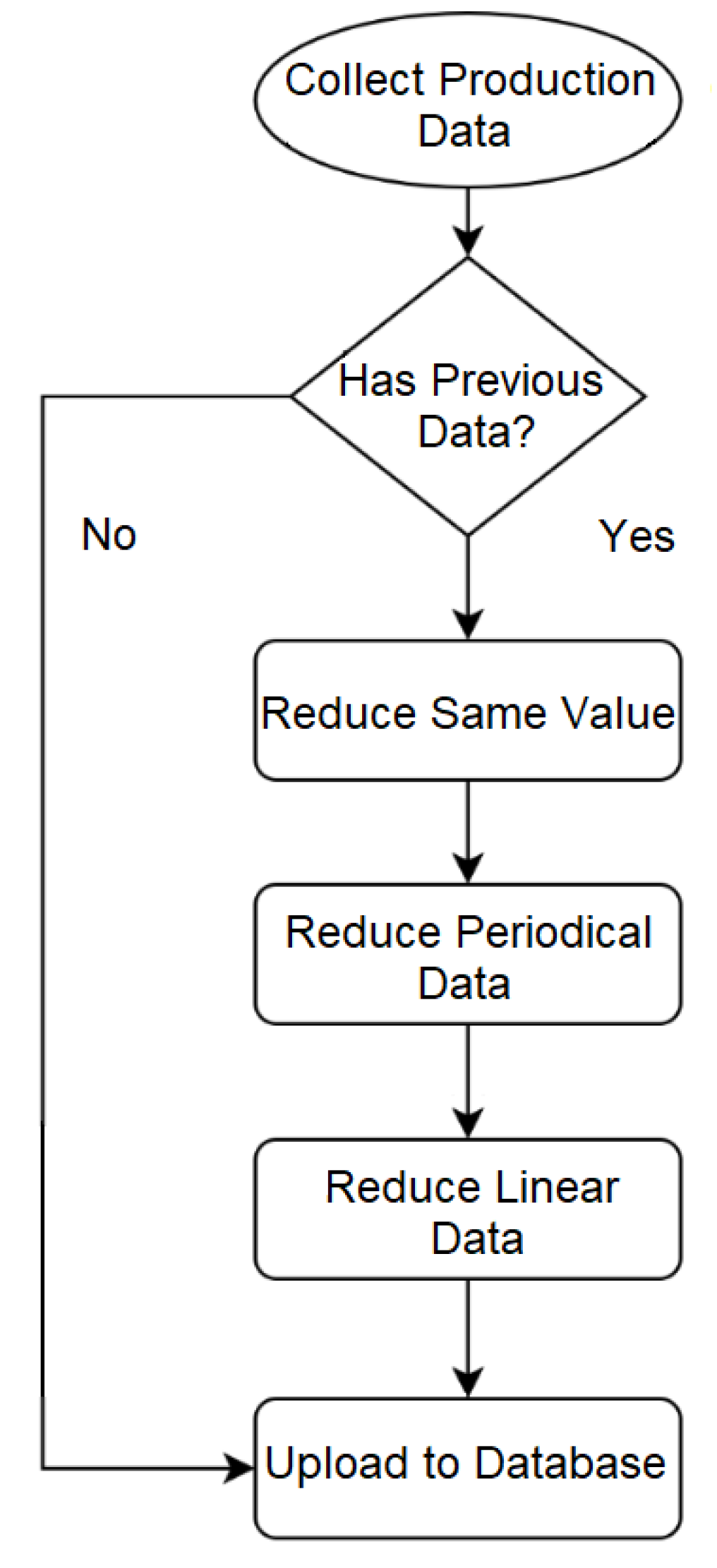
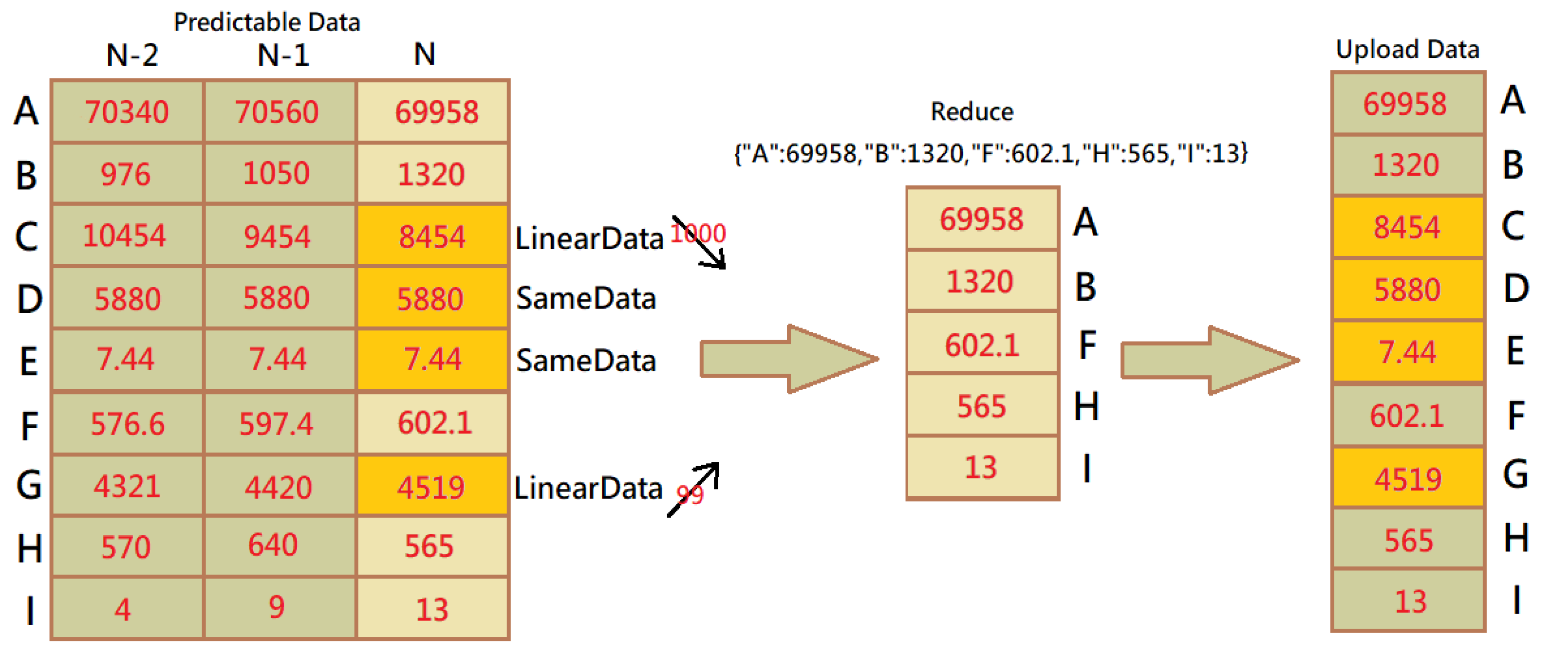
3.1. Reduced Data Transmission
3.2. High Accuracy Machine Status Analysis
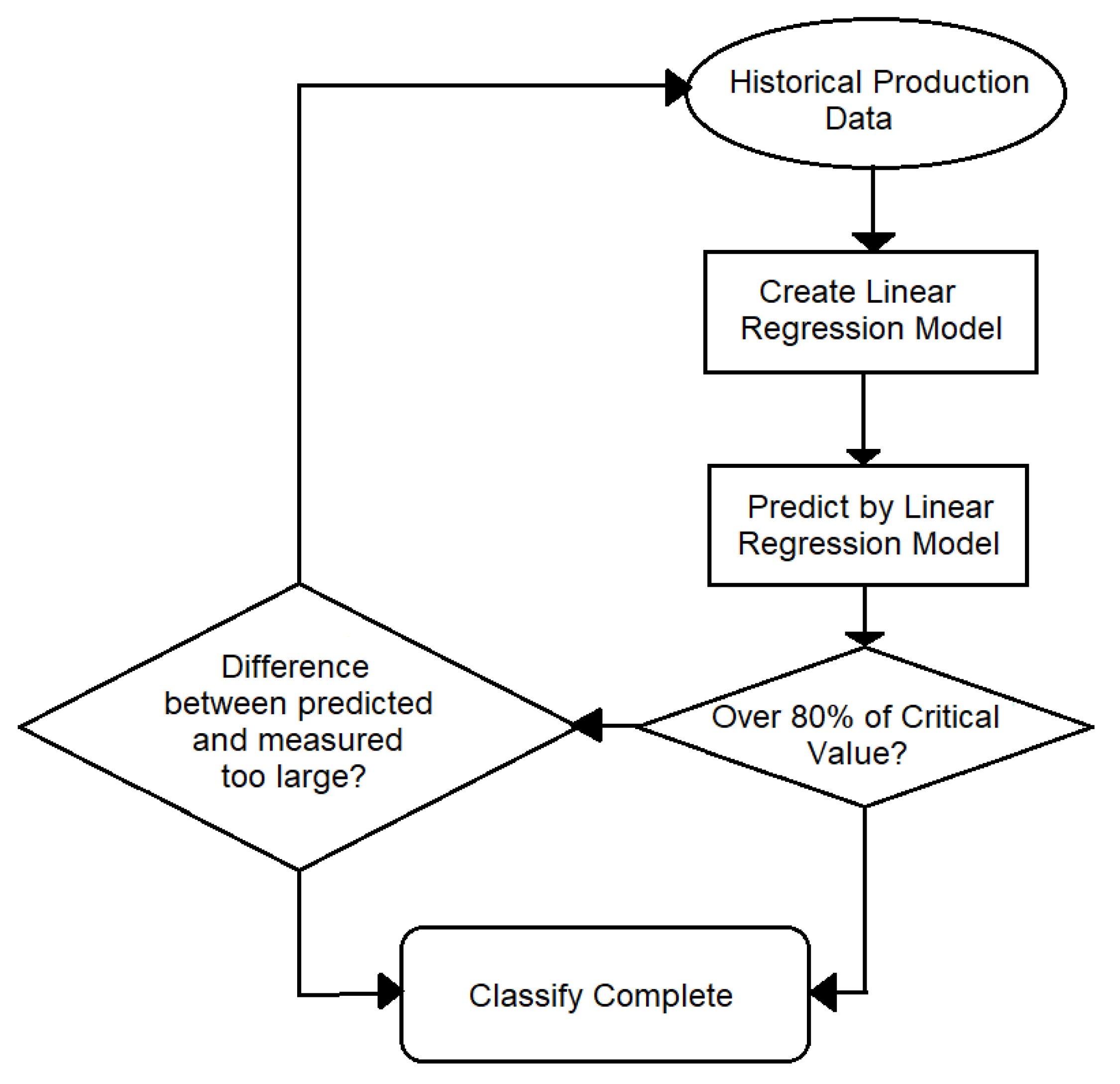
3.3. High Accuracy Machine Maintenance Prediction
4. Results and Discussion
4.1. Efficiency of Reducing Data Transmission
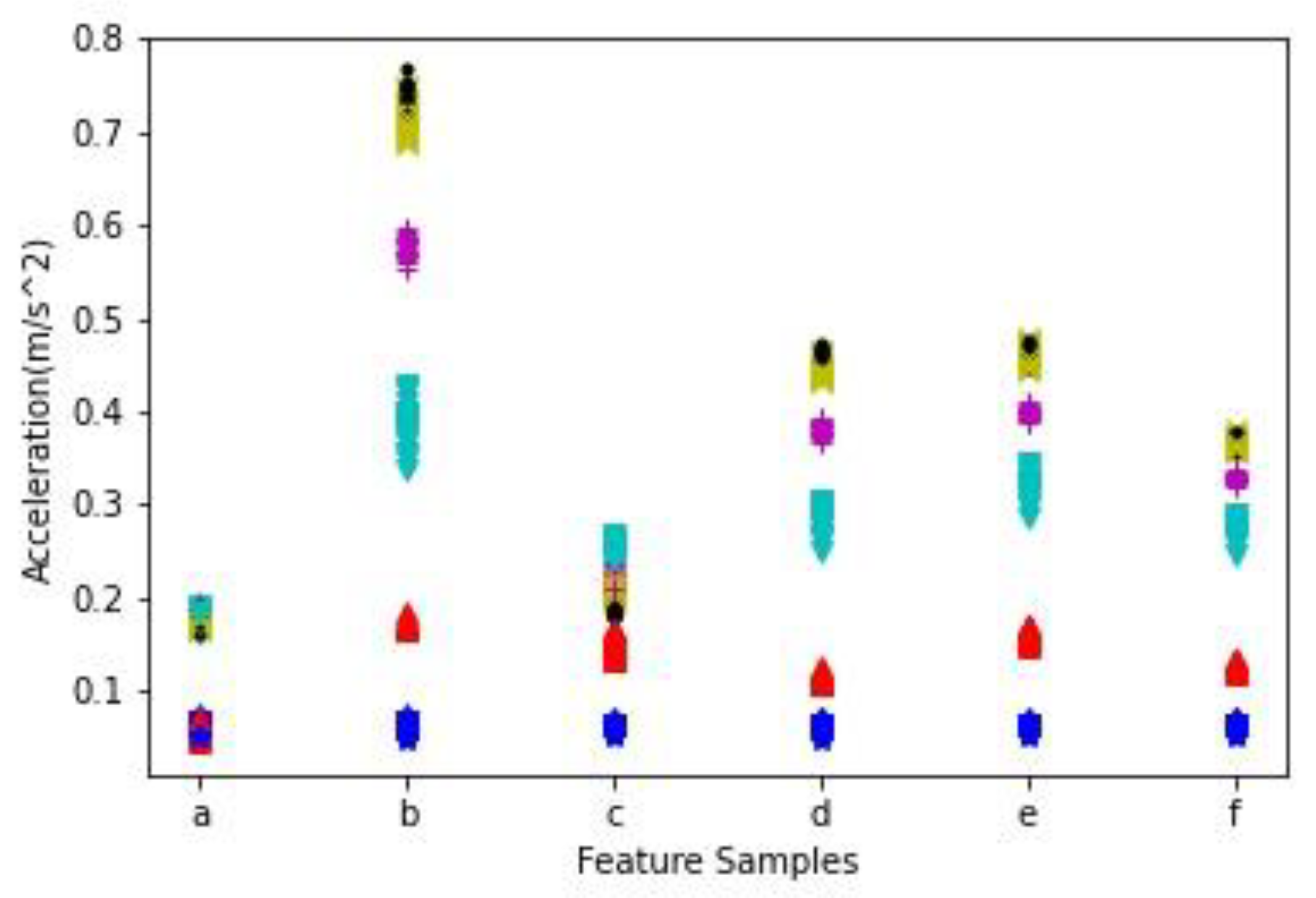
4.2. Accuracy of Machinery Status Analytics
4.3. Maintenance Prediction Analysis
5. Conclusions
Author Contributions
Funding
Data Availability Statement
Conflicts of Interest
References
- Narayanan, A.; Sena, A.; Gutierrez-Rojas, D.; Melgarejo, D.; Hussain, H.; Ullah, M.; Bayhan, S.; Nardelli, P. Key Advances in Pervasive Edge Computing for Industrial Internet of Things in 5G and Beyond. IEEE Access J. 2020, 8, 206734–206754. [Google Scholar] [CrossRef]
- Lin, C.; Su, X.; Yu, K.; Jian, B.; Yau, H. Inspection on Ball Bearing Malfunction by Chen-Lee Chaos System. IEEE Access J. 2020, 8, 28267–28275. [Google Scholar] [CrossRef]
- Saucedo-Dorantes, J.; Delgado-Prieto, M.; Osornio-Rios, R.; Romero-Troncoso, R. Industrial Data-driven Monitoring Based on Incremental Learning Applied to the Detection of Novel Faults. IEEE Trans. Ind. Inform. J. 2020. [Google Scholar] [CrossRef]
- Chu, Y.; Pham, T.; Hsu, F.; Tuw, M.; Tan, C.; Chay, M.; Lim, S.; Tsai, M. An effective method for monitoring the vibration data of bearings to diagnose and minimize defects. In Proceedings of the IASED International Joint Conference on Information and Communication Engineering, Shanghai, China, 27–29 April 2018; pp. 1–6. [Google Scholar]
- Peng, Y.; Qiao, W.; Qu, L.; Wang, J. Sensor Fault Detection and Isolation for a Wireless Sensor Network-Based Remote Wind Turbine Condition Monitoring System. IEEE Trans. Ind. Appl. J. 2017, 54, 1072–1079. [Google Scholar] [CrossRef]
- Khademi, A.; Raji, F.; Sadeghi, M. IoT enabled vibration monitoring toward smart maintenance. In Proceedings of the IEEE International Conference on Internet of Things and Applications, Isfahan, Iran, 17–18 April 2019; pp. 1–6. [Google Scholar]
- Muslewski1, L.; Pajak, M.; Grzadziela, A.; Musial, J. Analysis of Vibration Time Histories in the Time Domain for Propulsion Systems of Minesweepers. J. Vibroengineering 2015, 17, 1309–1316. [Google Scholar]
- Asalapuram, V.; Khan, I.; Rao, K. A novel architecture for condition based machinery health monitoring on marine vessels using deep learning and edge computing. In Proceedings of the IEEE International Symposium on Measurement and Control in Robotics, Houston, TX, USA, 19–21 September 2019; pp. 1–6. [Google Scholar]
- Yu, W.; Dillon, T.; Mostafa, F.; Rahayu, W.; Liu, Y. A global manufacturing big data ecosystem for fault detection in predictive maintenance. IEEE Trans. Ind. Inform. J. 2020, 16, 183–192. [Google Scholar] [CrossRef]
- Kim, D.; Lee, E.; Qureshi, N. Peak-Load Forecasting for Small Industries: A Machine Learning Approach. Sustainability 2020, 12, 6539. [Google Scholar] [CrossRef]
- Nayana, B.; Geethanjali, P. Analysis of Statistical Time-Domain Features Effectiveness in Identification of Bearing Faults from Vibration Signal. IEEE Sens. J. 2017, 17, 5618–5625. [Google Scholar] [CrossRef]
- Michal, P. Fuzzy Identification of a Threat of the Inability State Occurrence. J. Intell. Fuzzy Syst. 2018, 35, 3593–3604. [Google Scholar]
- Lin, Z.; Li, Y.; Liu, C.; Liao, I.; Hsieh, S.; Tsai, M. Machine maintenance management and repair prediction system. In Proceedings of the Mobile Computing Workshop, Tainan, Taiwan, China, 26–27 August 2018; pp. 1–3. [Google Scholar]
- Borith, T.; Bakhit, S.; Nasridinov, A.; Yoo, K. Prediction of Machine Inactivation Status Using Statistical Feature Extraction and Machine Learning. Appl. Sci. 2020, 10, 7413. [Google Scholar] [CrossRef]
- Saufi, S.; Ahmad, Z.; Leong, M.; Lim, M. Challenges and Opportunities of Deep Learning Models for Machinery Fault Detection and Diagnosis: A Review. IEEE Access J. 2019, 7, 122644–122662. [Google Scholar] [CrossRef]
- Huang, S.; Huang, J.; Huang, C.; Chen, J.; Liao, I.; Hsieh, S.; Tsai, M. Equipment component recognition cloud platform with information security. In Proceedings of the Workshop on Consumer Electronics, Yunlin, Taiwan, China, 29 November 2019; pp. 1–3. [Google Scholar]
- Gong, X.; Du, W.; Georgiadis, A.; Zhao, B. Identification of Multi-fault in Rotor-bearing System using Spectral Kurtosis and EEMD. J. Vibroengineering 2017, 19, 5036–5046. [Google Scholar] [CrossRef] [Green Version]
- Yu, F.; Fan, F.; Wang, S.; Zhou, F. Transform-domain Sparse Representation Based Classification for Machinery Vibration Signals. J. Vibroengineering 2018, 20, 979–987. [Google Scholar]
- Pajak, M. Identification of the Operating Parameters of a Complex Technical System Important from the Operational Potential Point of View. Proc. Inst. Mech. Eng. Part I J. Syst. Control Eng. 2018, 232, 62–78. [Google Scholar] [CrossRef] [Green Version]
- Angelopoulos, A.; Michailidis, E.; Nomikos, N.; Trakadas, P.; Hatziefremidis, A.; Voliotis, S.; Zahariadis, T. Tackling Faults in the Industry 4.0 Era—A Survey of Machine-Learning Solutions and Key Aspects. Sensors 2020, 20, 109. [Google Scholar] [CrossRef] [PubMed] [Green Version]
- Guo, R.; Zhao, Z.; Huo, S.; Jin, Z.; Zhao, J.; Gao, D. Research on State Recognition and Failure Prediction of Axial Piston Pump based on Performance Degradation Data. Process. J. 2020, 8, 609. [Google Scholar] [CrossRef]


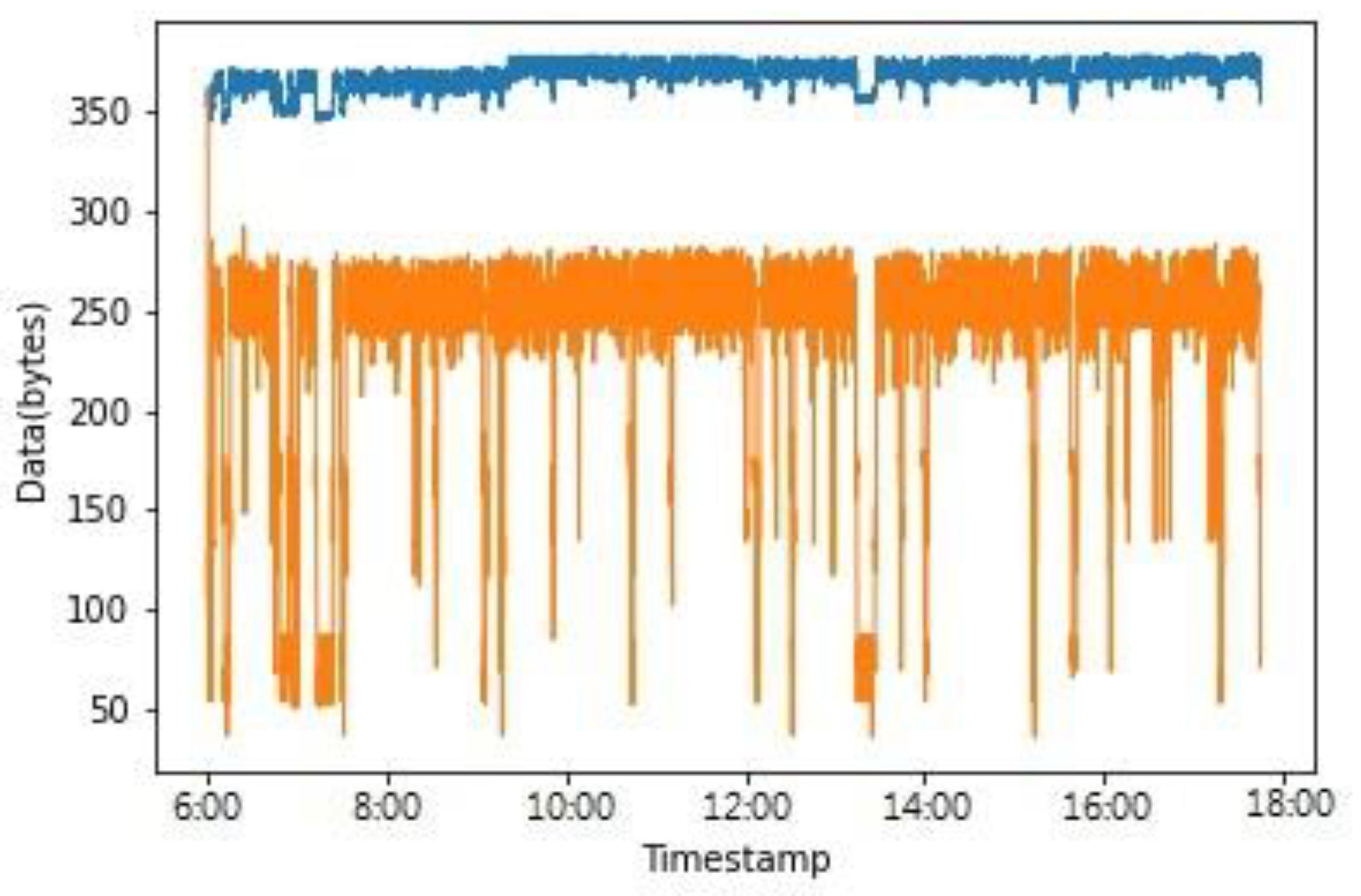
| Average upload length of each group of data (no algorithm) | 368 bytes |
| Average upload length of each group of data (with algorithm) | 233.8 bytes |
| Percentage reduction | 36.47% |
| Average upload length of each group of data (no algorithm) | 368 bytes |
| Average upload length of each group of data (with algorithm) | 167.2 bytes |
| Percentage reduction | 54.57% |
| The n Second | The n + 1 Second | The n + 2 Second | Avg of n, n + 1 | Avg of n + 1, n + 2 | Avg of all | Weight | |
|---|---|---|---|---|---|---|---|
| StandBy | 0.051349 | 0.054914 | 0.053374 | 0.053132 | 0.054144 | 0.053212 | 1/6 |
| Idling | 0.065304 | 0.174465 | 0.161900 | 0.119885 | 0.168183 | 0.133890 | 1/6 |
| Blowing I | 0.163742 | 0.338481 | 0.232462 | 0.251112 | 0.285472 | 0.244895 | 1/6 |
| Blowing II | 0.182730 | 0.567566 | 0.234054 | 0.375148 | 0.400810 | 0.328117 | 1/6 |
| Blowing III | 0.165524 | 0.696522 | 0.215582 | 0.431023 | 0.456052 | 0.359209 | 1/6 |
| Blowing IV | 0.175751 | 0.720361 | 0.203247 | 0.448056 | 0.461804 | 0.366453 | 1/6 |
| StandBy | 0.051349 | 0.054914 | 0.053374 | 0.053132 | 0.054144 | 0.053212 | 1/8 |
| Idling | 0.065304 | 0.174465 | 0.161900 | 0.119885 | 0.168183 | 0.133890 | 1/8 |
| Blowing I | 0.163742 | 0.338481 | 0.232462 | 0.251112 | 0.285472 | 0.244895 | 1/8 |
| Blowing II | 0.182730 | 0.567566 | 0.234054 | 0.375148 | 0.400810 | 0.328117 | 1/8 |
| Blowing III | 0.165524 | 0.696522 | 0.215582 | 0.431023 | 0.456052 | 0.359209 | 1/4 |
| Blowing IV | 0.175751 | 0.720361 | 0.203247 | 0.448056 | 0.461804 | 0.366453 | 1/4 |
| StandBy | 0.051349 | 0.054914 | 0.053374 | 0.053132 | 0.054144 | 0.053212 | 1/10 |
| Idling | 0.065304 | 0.174465 | 0.161900 | 0.119885 | 0.168183 | 0.133890 | 1/10 |
| Blowing I | 0.163742 | 0.338481 | 0.232462 | 0.251112 | 0.285472 | 0.244895 | 1/10 |
| Blowing II | 0.182730 | 0.567566 | 0.234054 | 0.375148 | 0.400810 | 0.328117 | 1/6 |
| Blowing III | 0.165524 | 0.696522 | 0.215582 | 0.431023 | 0.456052 | 0.359209 | 1/3 |
| Blowing IV | 0.175751 | 0.720361 | 0.203247 | 0.448056 | 0.461804 | 0.366453 | 1/5 |
| Feature Sample | ||||||
|---|---|---|---|---|---|---|
| The n Second | The n + 1 Second | The n + 2 Second | Avg of n, n + 1 | Avg of n + 1, n + 2 | Avg of all | |
| Blowing I | 0.163742 | 0.338481 | 0.232462 | 0.251112 | 0.285472 | 0.244895 |
| Blowing IV | 0.175751 | 0.720361 | 0.203247 | 0.448056 | 0.461804 | 0.366453 |
| Blowing IV | 0.171148 | 0.731996 | 0.184157 | 0.451572 | 0.458077 | 0.362434 |
| Blowing IV | 0.176430 | 0.736780 | 0.187903 | 0.456605 | 0.462342 | 0.367038 |
| Blowing IV | 0.180478 | 0.736250 | 0.185272 | 0.458364 | 0.460761 | 0.367333 |
| Blowing IV | 0.179346 | 0.725493 | 0.193486 | 0.452420 | 0.459490 | 0.366108 |
| Feature Sample | ||||||
|---|---|---|---|---|---|---|
| The n Second | The n + 1 Second | The n + 2 Second | Avg of n, n + 1 | Avg of n + 1, n + 2 | Avg of all | |
| Blowing I | 0.163742 | 0.338481 | 0.232462 | 0.251112 | 0.285472 | 0.244895 |
| Blowing III | 0.182643 | 0.721272 | 0.201569 | 0.451958 | 0.461421 | 0.368495 |
| Blowing III | 0.167709 | 0.716777 | 0.201444 | 0.442243 | 0.459111 | 0.361977 |
| Blowing III | 0.165524 | 0.696522 | 0.215582 | 0.431023 | 0.456052 | 0.359209 |
| Blowing III | 0.168686 | 0.724333 | 0.207251 | 0.446510 | 0.465792 | 0.366757 |
| Blowing IV | 0.179346 | 0.725493 | 0.193486 | 0.452420 | 0.459490 | 0.366108 |
| The n Second | The n + 1 Second | The n + 2 Second | Avg of n, n + 1 | Avg of n + 1, n + 2 | Avg of all | |
|---|---|---|---|---|---|---|
| StandBy | 0.051349 | 0.054914 | 0.053374 | 0.053132 | 0.054144 | 0.053212 |
| Idling | 0.065304 | 0.174465 | 0.161900 | 0.119885 | 0.168183 | 0.133890 |
| Blowing I | 0.163742 | 0.338481 | 0.232462 | 0.251112 | 0.285472 | 0.244895 |
| Blowing II | 0.182730 | 0.567566 | 0.234054 | 0.375148 | 0.400810 | 0.328117 |
| Blowing III | 0.165524 | 0.696522 | 0.215582 | 0.431023 | 0.456052 | 0.359209 |
| Blowing IV | 0.175751 | 0.720361 | 0.203247 | 0.448056 | 0.461804 | 0.366453 |
| Feature Sample | ||||||
| Blowing III | 0.167709 | 0.716777 | 0.201444 | 0.442243 | 0.459111 | 0.361977 |
| Methods | KNN | Adaboost | Naïve Bayes | Decision Tree | Random Forest | Non-linear SVM |
|---|---|---|---|---|---|---|
| Accuracies | 93% | 96% | 93% | 90% | 93% | 98% |
Publisher’s Note: MDPI stays neutral with regard to jurisdictional claims in published maps and institutional affiliations. |
© 2020 by the authors. Licensee MDPI, Basel, Switzerland. This article is an open access article distributed under the terms and conditions of the Creative Commons Attribution (CC BY) license (http://creativecommons.org/licenses/by/4.0/).
Share and Cite
Tsai, M.-F.; Chu, Y.-C.; Li, M.-H.; Chen, L.-W. Smart Machinery Monitoring System with Reduced Information Transmission and Fault Prediction Methods Using Industrial Internet of Things. Mathematics 2021, 9, 3. https://doi.org/10.3390/math9010003
Tsai M-F, Chu Y-C, Li M-H, Chen L-W. Smart Machinery Monitoring System with Reduced Information Transmission and Fault Prediction Methods Using Industrial Internet of Things. Mathematics. 2021; 9(1):3. https://doi.org/10.3390/math9010003
Chicago/Turabian StyleTsai, Ming-Fong, Yen-Ching Chu, Min-Hao Li, and Lien-Wu Chen. 2021. "Smart Machinery Monitoring System with Reduced Information Transmission and Fault Prediction Methods Using Industrial Internet of Things" Mathematics 9, no. 1: 3. https://doi.org/10.3390/math9010003