Estimation of Unknown Parameters of Truncated Normal Distribution under Adaptive Progressive Type II Censoring Scheme

Abstract

In reality, estimations for the unknown parameters of truncated distribution with censored data have wide utilization. Truncated normal distribution is more suitable to fit lifetime data compared with normal distribution. This article makes statistical inferences on estimating parameters under truncated normal distribution using adaptive progressive type II censored data. First, the estimates are calculated through exploiting maximum likelihood method. The observed and expected Fisher information matrices are derived to establish the asymptotic confidence intervals. Second, Bayesian estimations under three loss functions are also studied. The point estimates are calculated by Lindley approximation. Importance sampling technique is applied to discuss the Bayes estimates and build the associated highest posterior density credible intervals. Bootstrap confidence intervals are constructed for the purpose of comparison. Monte Carlo simulations and data analysis are employed to present the performances of various methods. Finally, we obtain optimal censoring schemes under different criteria.

1. Introduction

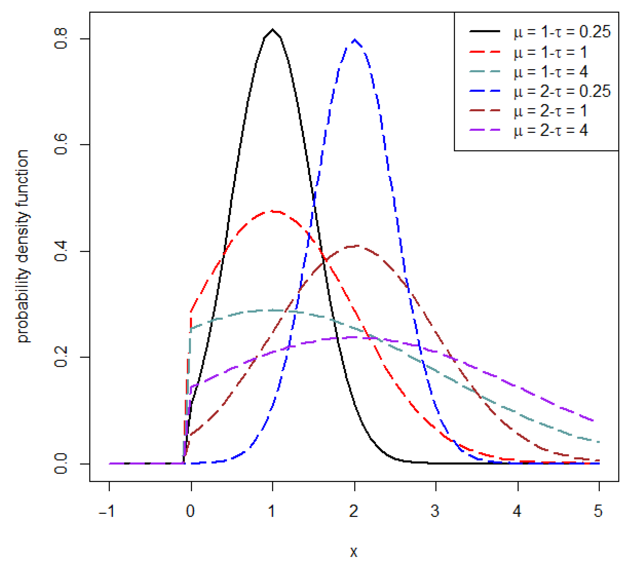
1.1. Truncated Normal Distribution

Normal distribution is one of the most significant probability distributions in statistics on account that it fits lots of natural phenomena. With its satisfactory performance on fitting data and nice properties, analysts always discuss the characteristics of data based on normal distribution. However, negative data seldom appear in most cases of reality such as life test experiments. To overcome this, truncation is introduced to limit the values within a specific scope, which fits the data better so that the final analytical results after computations and estimations will be more accurate. Thus, truncated normal distribution, restricting the domain of normal distribution between one or two bounds, can be found to have theoretical and practical values.

Truncated normal distribution has not received extensive attention in academia until recent years for the complexity of its numeric characteristics when making statistical inferences. Based on this distribution, Ref. [1] compared the maximum likelihood estimations of mean and variance under censored samples with complete samples. Moreover, using the progressive type-II censoring model, Ref. [2] estimated the parameters of left truncated normal distribution. On the aspect of applications, Ref. [3] approximated the length of queue with abandonment based on truncated normal distribution. So far, studies related to this distribution still leave plenty of space to explore.

In this article, a normal distribution that is left truncated at zero is investigated. We denote it as $TN(\mu ,\tau )$ for convenience. Notice that $\mu ,\tau$ are the parameters of mean and variance. The corresponding probability density function (pdf) is described as

$$\begin{array}{c}\hfill f(x;\mu ,\tau )=\frac{e^{-\frac{1}{2\tau }{(x-\mu )}^2}}{\sqrt{2\pi \tau }\Phi (\frac{\mu }{\sqrt{\tau }})},x,\mu ,\tau >0,\end{array}$$

(1)

and the cumulative distribution function (cdf) is written as

$$\begin{array}{c}\hfill F(x;\mu ,\tau )=1-\frac{1-\Phi (\frac{x-\mu }{\sqrt{\tau }})}{\Phi (\frac{\mu }{\sqrt{\tau }})}.\end{array}$$

(2)

Here $\Phi (·)$ represents the cdf of standard normal distribution. The survival function can be written as

$$\begin{array}{c}\hfill S(x;\mu ,\tau )=1-F(x;\mu ,\tau )=\frac{1-\Phi (\frac{x-\mu }{\sqrt{\tau }})}{\Phi (\frac{\mu }{\sqrt{\tau }})}.\end{array}$$

(3)

Figure 1 reflects that the truncated normal distribution pdf is unimodal. Similar to normal distribution, as $\mu$ increases, location of truncated normal distribution moves along the right direction while the shape becomes narrower and sharper as $\tau$ decreases. However, because of truncation, the density location change is no longer a translation under the condition that the variance is fixed. Instead, the value of pdf becomes lower as $\mu$ moves away from the truncated point in positive direction. Figure 2 presents some characteristics of cdf. The fastest increasing point among all points in the domain appears at the mean. The growth of cdf becomes slower with $\tau$ decreasing. Furthermore, larger $\mu$ leads to lower rising rate.

In general, we denote a random variable following truncated normal distribution as X and assume that this distribution is left truncated at a. Different from normal distribution random variable, the expectation and variance of X are not only determined on the parameters $\mu$ and $\tau$ but also depended on the truncated point. According to [4], the expectation is $E(X)=\mu +\sqrt{\tau }\frac{\varphi (\alpha )}{1-\Phi (\alpha )}$ and variance is $Var(X)=\tau [1+\frac{\alpha \varphi (\alpha )}{1-\Phi (\alpha )}-{(\frac{\varphi (\alpha )}{1-\Phi (\alpha )})}^2]$, where $\alpha =\frac{a-\mu }{\tau }$. Meanwhile, the characteristic function is given as $\chi (t)=e^{i\mu t-\frac{1}{2}\tau t^2}[\frac{1-\Phi (\alpha -it\sqrt{\tau })}{1-\Phi (\alpha )}]$ and the moment generating function is $M(t)=e^{\mu t+\frac{1}{2}\tau t^2}[\frac{1-\Phi (\alpha -t\sqrt{\tau })}{1-\Phi (\alpha )}]$, which are helpful to calculate the moments.

Particularly, if $a=0$, its expectation, variance, characteristic function, as well as moment generating function are expressed separately as

$$\begin{array}{ccc}\hfill E(X;\mu ,\tau )& =& \mu +\sqrt{\tau }\frac{\frac{\mu }{\sqrt{\tau }}}{\Phi (\frac{\mu }{\sqrt{\tau }})},\hfill \end{array}$$

(4)

$$\begin{array}{ccc}\hfill Var(X;\mu ,\tau )& =& \tau [1-\frac{\mu }{\sqrt{\tau }}\frac{\varphi (\frac{\mu }{\sqrt{\tau }})}{\Phi (\frac{\mu }{\sqrt{\tau }})}-(\frac{\varphi (\frac{\mu }{\sqrt{\tau }})}{\Phi (\frac{\mu }{\sqrt{\tau }})}{)}^2],\hfill \end{array}$$

(5)

$$\begin{array}{ccc}\hfill \chi (X;\mu ,\tau )& =& e^{i\mu t-\frac{1}{2}{t}^2\tau }[\frac{\Phi (\frac{\mu }{\sqrt{\tau }}+it\sqrt{\tau })}{\Phi (\frac{\mu }{\sqrt{\tau }})}],\hfill \end{array}$$

(6)

$$\begin{array}{ccc}\hfill M(X;\mu ,\tau )& =& e^{\mu t+\frac{1}{2}{t}^2\tau }[\frac{\Phi (\frac{\mu }{\sqrt{\tau }}+t\sqrt{\tau })}{\Phi (\frac{\mu }{\sqrt{\tau }})}].\hfill \end{array}$$

(7)

1.2. Adaptive Progressive Type-II Censored Scheme

In survival analysis and reliability test, incomplete observation is a universal problem perplexing lots of scholars for the limitation of time and cost. Thus, censored schemes are applied to improve the efficiency of experiments. Various censoring schemes are put forward and studied by many statisticians. Type I and II censoring have found the most universal applications among these censoring models. In type-I censoring, the life span experiment stops at a prefixed time and the units remaining are right censored while under type-II censoring, m, the number of failures is predetermined and the experiment stops once the m-th failure happens. However, being unable to remove the survival units during the test is one of the weaknesses in the two censoring schemes. To conquer this, progressive type II censoring model was proposed. In this scheme, there are totally n sample units in an experiment. On the occurrence of the first failure, $R_1$ live units are removed at random from $n-1$ live units remaining. Similarly, from remaining $n-j-{\sum }_{i=1}^{j-1}{R}_i$ units remove $R_j$ units when the j-th failure appears. This process is ongoing until m-th failure happens. Here the failure time of m units are described as $X_{(1:m:n)},\cdots ,X_{(m-1:m:n)},X_{(m:m:n)}$. In addition, $(R_1,\cdots ,R_{m-1},R_m)$ represents the censoring scheme. Note that the number m and censoring scheme are prescribed at the beginning. Readers who are interested in progressive censoring can consult [5,6] for further information.

However, progressive type II censoring scheme is lack of flexibility. For example, during the life testing experiment, researchers may want to control the experiment time accordingly under the practical condition. Adaptive progressive type-II censored scheme is proposed to deal with that problem. This scheme is implemented in sequel. At the start of a life test experiment with n units totally, m, the size of observed units and $(R_1,\cdots ,R_{m-1},R_m)$ are predetermined. In addition, T, the expected total testing time, is preprovided by researchers. Before T, this test is carried out according to the censoring plan which is given in advance like progressive type II censoring. However, once the actual time runs over T, researchers tend to obtain more observations in a shorter time by leaving more live units. The survival units would no longer be removed until the m-th failure appears. Assume that the practical test time exceeds over T exactly right after the J-th failure happens. (i.e., $X_{(J:m:n)}<T<X_{(J+1:m:n)},X_{(m+1:m:n)}\equiv \infty ,X_{(0:m:n)}\equiv 0,J=0,1,\cdots ,m.$). Therefore, when the actual time overruns T, the censoring scheme in the following becomes $R_m=n-m-{\sum }_{i=1}^J{R}_i$ and $R_{J+1}=R_{J+2}=\cdots =R_{m-2}=R_{m-1}=0$. Particularly, on condition that T is equal to 0, this scheme turns into conventional type-II censoring scheme. If the time of test is sufficient, $T=\infty$ is the corresponding premise. This model eventually changes to progressive type-II censoring model.

Considering the limitations of time and efficiency in practical situations, adaptive progressive type-II censoring censoring scheme enables researchers to control the experiment with flexibility in the process. This good property has attracted more and more scholars to do correlative investigation. Ref. [7] first proposed adaptive progressive type-II censoring model. Under the one- and two-parameter exponential distribution, Ref. [8] elaborated inferences related to estimating unknown parameters on the basis of this censoring scheme. Ref. [6] introduced the concepts of this censoring model and illustrated other related models in detail. Ref. [9] extended this censoring model by considering competing risks under exponential distribution and presented statistical inferences. On the basis of this scheme, Ref. [10] estimated the unknown parameters of a special distribution whose failure rate function is bathtub-shaped through maximum likelihood estimation and Bayesian approach.

For estimation methods, classical statistics and Bayesian inference are the mainstream approaches. Maximum likelihood estimation has been widely used as an important classical method of estimation. The life of experiment units are assumed to follow a certain lifetime distribution and be independent and identically distributed (i.i.d.). Then the maximum likelihood estimates are computed through maximizing the likelihood function. However, the small sample size leads to inaccurate estimation under this method. Bayesian estimation tackles this disadvantage by incorporating prior knowledge. Given the probability density function of sample and the prior distribution of parameters, Bayes estimates are obtained by calculating the expected value under posterior distribution. However, improper prior distribution selection may cause large errors and there is a certain degree of subjectivity in selection. Hence, giving careful consideration to choose prior distribution is very significant. In addition, the integral is difficult to be computed in Bayes estimation sometimes; importance sampling is a suitable approach to perform numerical calculations with an easily sampled distribution.

This paper aims to study estimation problems for the truncated normal distribution parameters under adaptive progressive type II censoring model. Both point estimations and interval estimations are discussed by applying classical approaches and Bayesian methods. Here the same distribution with Lodhi et al. (2019) is considered, but we mainly focus on enriching Bayesian estimation section and choosing three kinds of loss functions to calculate, which is comprehensive and comparable. Under the more flexible and complex censoring model, deducing functions, taking derivatives and writing codes to make simulations are more difficult. In addition, some evidences are needed before employing methods are proved, making this article rigorous.

In Section 2, via Newton–Raphson method, the maximum likelihood estimates of the truncated normal distribution parameters are obtained. Meanwhile, observed Fisher matrix is computed to build the corresponding aymptotic confidence intervals. Furthermore, the distribution of the j-th failure and expected Fisher information matrix are also discussed. Section 3 carrys out Bayesian estimations under different loss functions including square error loss Function (SELF), Linex loss function (LLF) and general entropy loss function (GELF). Lindley approximation and importance sampling are mainly adopted to calculate the estimates of parameters. On the basis of that, highest posterior density credible intervals (HPD intervals) are also established. Meanwhile, bootstrap confidence intervals are constructed in accordance with the algorithm steps in Section 4. In Section 5, the results obtained with different methods are compared and evaluated by carrying out simulations. To illustrate the effectiveness of estimation methods, analysis on a real data set are carried out in Section 6. Furthermore, Section 7 investigates the problem of selecting optimal censoring scheme under adaptive type II censored model. Eventually, Section 8 summarizes the whole article.

2. Maximum Likelihood Estimation

The estimators are derived in this section from the perspective of point estimation and interval estimation by utilizing maximum likelihood method. The equations inferred from likelihood function to obtain the estimates are demonstrated. Through observed Fisher information matrix, we also construct asymptotic confidence intervals. Some inferences about expected Fisher matrix are also presented in sequel. Assume that $X_{(1:m:n)},\cdots ,X_{(m-1:m:n)},X_{(m:m:n)}$ represent the censored sample under the prefixed censoring plan $(R_1,\cdots ,R_{m-1},R_m)$ and the ideal total time is provided as T. In particular, before T, the last failure occurs at $X_{J:m:n}$. For the sake of simplicity, $X_{(1:m:n)},\cdots ,X_{(m-1:m:n)},X_{(m:m:n)}$ are denoted respectively by $X_{(1)},\cdots ,X_{(m-1)},X_{(m)}$.

2.1. Point Estimation

Suppose that the failure data $x_{(1)},\cdots ,x_{(m-1)},x_{(m)}$ are observed in the experiment. Let $\underline{x}$ represent the observed data ($x_{(1)},\cdots ,x_{(m-1)},x_{(m)}$). Given the pdf $f(x)$, the cdf $F(x)$ and the J which is obtained by setting T in advance, the likelihood function is described as

$$\begin{array}{c}\hfill L(\underline{x})=D_J[1-F(x_{(m)}){]}^{(n-m-{\sum }_{i=1}^J{R}_i)}[\prod _{i=1}^{m}f(x_{(i)})\left]\right\{\prod _{i=1}^J{[1-F(x_{(i)})]}^{R_i}\},\end{array}$$

(8)

where

$$D_J=\prod _{i=1}^m[n+1-i-\sum _{k=1}^{max\{J,i-1\}}{R}_k].$$

In the situation that data are subject to truncated normal distribution, $f(x)$ and $F(x)$ are the pdf and cdf of $TN(\mu ,\tau )$ separately. The corresponding likelihood function and log-likelihood function are expressed by

$$\begin{array}{c}\hfill L(\mu ,\tau |\underline{x})=D_J\left[\prod _{i=1}^m\frac{e^{-\frac{{\xi }_{x_{(i)}}^2}{2}}}{\sqrt{2\pi \tau }\Phi (\xi )}\right]\left\{\prod _{i=1}^J{[\frac{1-\Phi ({\xi }_{x_{(i)}})}{\Phi (\xi )}]}^{R_i}\right\}{[\frac{1-\Phi ({\xi }_{x_{(m)}})}{\Phi (\xi )}]}^{(n-m-{\sum }_{i=1}^J{R}_i)},\end{array}$$

(9)

$$\begin{array}{ccc}\hfill lnL(\mu ,\tau )& =& \mathrm{constant}-\frac{1}{2}\sum _{i=1}^{m}ln\tau -nln\Phi (\xi )+\sum _{i=1}^J{R}_i[ln(1-\Phi ({\xi }_{x_{(i)}}))]\hfill \\ & +& (n-m-\sum _{i=1}^J{R}_i)[ln(1-\Phi ({\xi }_{x_{(m)}}))],\hfill \end{array}$$

(10)

where $\xi =\frac{\mu }{\sqrt{\tau }}$, ${\xi }_{x_{(i)}}=\frac{x_{(i)}-\mu }{\sqrt{\tau }}$ and $\varphi (·)$ is the pdf of standard normal distribution. $\widehat{\mu }$ and $\widehat{\tau }$ are used to denote the MLEs of $\mu$ and $\tau$. For the purpose of obtaining corresponding $\widehat{\mu }$ and $\widehat{\tau }$, the partial derivatives of likelihood function for $\mu$ and $\tau$ are set to be equal to 0. $\widehat{\mu }$ and $\widehat{\tau }$ are calculated by solving the equations, which maximizes the likelihood function. Then the equations are given as follows

$$\begin{array}{ccc}\hfill \frac{\partial lnL(\mu ,\tau )}{\partial \mu }& =& \frac{1}{\sqrt{\tau }}[\sum _{i=1}^m{\xi }_{x_{(i)}}-\frac{n\varphi (\xi )}{\Phi (\xi )}+\sum _{i=1}^J{R}_i\frac{\varphi ({\xi }_{x_{(i)}})}{1-\Phi ({\xi }_{x_{(i)}})}\hfill \\ & +& (n-m-\sum _{i=1}^J{R}_i)\frac{\varphi ({\xi }_{x_{(m)}})}{1-\Phi ({\xi }_{x_{(m)}})}]=0,\hfill \end{array}$$

(11)

$$\begin{array}{ccc}\hfill \frac{\partial lnL(\mu ,\tau )}{\partial \tau }& =& \frac{1}{2\tau }[\sum _{i=1}^m{\xi }_{x_{(i)}}^2-m+n\xi \frac{\varphi (\xi )}{\Phi (\xi )}+\sum _{i=1}^J\frac{R_i{\xi }_{x_{(i)}}\varphi ({\xi }_{x_{(i)}})}{1-\Phi ({\xi }_{x_{(i)}})}\hfill \\ & +& (n-m-\sum _{i=1}^J{R}_i)\frac{{\xi }_{x_{(m)}}\varphi ({\xi }_{x_{(m)}})}{1-\Phi ({\xi }_{x_{(m)}})}]=0.\hfill \end{array}$$

(12)

Theorem 1.

When μ is given, the MLE of τ exists.

Proof. 

Please see Appendix A.  □

However, under this circumstance the Equations (11) and (12) are nonlinear and have no closed form solution. The denominators in the equations contain complex and nonlinear functions. They cannot be simplified. It is impossible to get the analytic solutions. So numerical techniques are essential to be introduced in order to settle this problem. Here to obtain the final estimates $\widehat{\mu }$ and $\widehat{\tau }$, Newton–Raphson method is chosen, which can be achieved by R software.

2.2. Asymptotic Confidence Interval

Aiming at constructing the approximate intervals of the two parameters, asymptotic variance-covariance matrix of $\widehat{\mu }$ and $\widehat{\tau }$ is discussed by performing Fisher information matrix inversion.

Through taking the expectation of the negative second derivative of the log-likelihood function, Fisher information matrix can be calculated. Thus it can be expressed as

$$\begin{array}{c}\hfill I(\mu ,\tau )=-E\left[\begin{array}{cc}\frac{{\partial }^{2}l\left(\mu ,\tau \right)}{\partial {\mu }^2}& \frac{{\partial }^{2}l\left(\mu ,\tau \right)}{\partial \mu \partial \tau }\\ \frac{{\partial }^{2}l\left(\mu ,\tau \right)}{\partial \tau \partial \mu }& \frac{{\partial }^{2}l\left(\mu ,\tau \right)}{\partial {\tau }^2}\end{array}\right].\end{array}$$

2.2.1. Observed Fisher Information Matrix

The observed Fisher matrix obtained based on samples is helpful and convenient to estimate the intervals of $\widehat{\mu }$ and $\widehat{\tau }$. For truncated normal distribution, it can be given as

$$\begin{array}{c}\hfill I(\widehat{\mu },\widehat{\tau })=\left[\begin{array}{cc}{a}_{11}& a_{12}\\ a_{21}& a_{22}\end{array}\right],\end{array}$$

where

$$\begin{array}{ccc}\hfill a_{11}& =& \frac{1}{\tau }[m+n{A}_{11}(\xi )+\sum _{i=1}^J{R}_i{A}_{11(i)}({\xi }_{x_{(i)}})+(n-m-\sum _{i=1}^J{R}_i)A_{11(m)}({\xi }_{x_{(m)}})],\hfill \\ \hfill a_{12}& =& a_{21}=\frac{1}{2\tau \sqrt{\tau }}[2\sum _{i=1}^m{\xi }_{x_{(i)}}+n{A}_{12}(\xi )+\sum _{i=1}^J{R}_i{A}_{12(i)}({\xi }_{x_{(i)}})+(n-m-\sum _{i=1}^J{R}_i)A_{12(m)}({\xi }_{x_{(m)}})],\hfill \\ \hfill a_{22}& =& \frac{1}{4{\tau }^2}[4\sum _{i=1}^J{\xi }_{x_{(i)}}^2-2m+n{A}_{22}(\xi )+\sum _{i=1}^J{R}_i{A}_{22(i)}({\xi }_{x_{(i)}})+(n-m-\sum _{i=1}^J{R}_i)A_{22(m)}({\xi }_{x_{(m)}})],\hfill \end{array}$$

and

$$\begin{array}{ccc}\hfill A_{11}(\xi )& =& -Q^2(\xi )+Q^{{}^{\prime }}(\xi ),\hfill \\ \hfill A_{12}(\xi )& =& -Q(\xi )-\xi Q^{{}^{\prime }}(\xi )+\xi Q^2(\xi ),\hfill \\ \hfill A_{22}(\xi )& =& 3\xi Q(\xi )+{\xi }^2{Q}^{{}^{\prime }}(\xi )-{\xi }^2{Q}^2(\xi ),\hfill \\ \hfill A_{11(i)}({\xi }_{x_{(i)}})& =& P_i^{{}^{\prime }}({\xi }_{x_{(i)}})+P_i^2({\xi }_{x_{(i)}}),\hfill \\ \hfill A_{12(i)}({\xi }_{x_{(i)}})& =& P_{(i)}({\xi }_{x_{(i)}})+{\xi }_{x_{(i)}}{P}_{(i)}^{{}^{\prime }}({\xi }_{x_{(i)}})+{\xi }_{x_{(i)}}{P}_{(i)}^2({\xi }_{x_{(i)}}),\hfill \\ \hfill A_{22(i)}({\xi }_{x_{(i)}})& =& 3{\xi }_{x_{(i)}}{P}_{(i)}({\xi }_{x_{(i)}})+{\xi }_{x_{(i)}}^2{P}_{(i)}^{{}^{\prime }}({\xi }_{x_{(i)}})+{\xi }_{x_{(i)}}^2{P}_{(i)}^2({\xi }_{x_{(i)}}),\hfill \end{array}$$

$\xi =\frac{\mu }{\sqrt{\tau }},{\xi }_{x_{(i)}}=\frac{x_{(i)}-\mu }{\sqrt{\tau }},Q(\xi )=\frac{\varphi (\xi )}{\Phi (\xi )},P_{(i)}({\xi }_{x_{(i)}})=\frac{\varphi ({\xi }_{x_{(i)}})}{1-\Phi ({\xi }_{x_{(i)}})},Q^{{}^{\prime }}(\xi )=\frac{{\varphi }^{{}^{\prime }}(\xi )}{\Phi (\xi )},P_{(i)}^{{}^{\prime }}({\xi }_{x_{(i)}})=\frac{{\varphi }^{{}^{\prime }}({\xi }_{x_{(i)}})}{1-\Phi ({\xi }_{x_{(i)}})},Q^2(\xi )={\left[\frac{\varphi (\xi )}{\Phi (\xi )}\right]}^2,P_{(i)}^2({\xi }_{x_{(i)}})={\left[\frac{\varphi ({\xi }_{x_{(i)}})}{1-\Phi ({\xi }_{x_{(i)}})}\right]}^2$, and ${\varphi }^{{}^{\prime }}(·)$ is the first derivative of the pdf of standard normal distribution. Then the associated variance-covariance matrix is described as

$$\begin{array}{c}\hfill Var(\widehat{\mu },\widehat{\tau })=\left[\begin{array}{cc}{\sigma }_{11}& {\sigma }_{12}\\ {\sigma }_{21}& {\sigma }_{22}\end{array}\right]={\left[\begin{array}{cc}{a}_{11}& a_{12}\\ a_{21}& a_{22}\end{array}\right]}^{-1}.\end{array}$$

(13)

Thus, the $100\%(1-\alpha )$ asymptotic confidence intervals are constructed separately as $(\widehat{\mu }-z_{\frac{\alpha }{2}}\sqrt{{\sigma }_{11}},\widehat{\mu }+z_{\frac{\alpha }{2}}\sqrt{{\sigma }_{11}})$ and $(\widehat{\tau }-z_{\frac{\alpha }{2}}\sqrt{{\sigma }_{22}},\widehat{\tau }+z_{\frac{\alpha }{2}}\sqrt{{\sigma }_{22}})$, where $z_{\alpha /2}$ is the $\frac{\alpha }{2}$-th percentile of the standard normal distribution.

2.2.2. Expected Fisher Information Matrix

Before experiment, $n,m,R,T$ are predetermined. J is the order of failure right after the time point T. So it is relevant to T and the actual process of test. Because of the randomness of the life testing experiment, only when the test is over can we get the exact value of J. Thus J can be treated as a random variable. However, unknown J leads to the difficulty of obtaining the expectation expression for the pdf of experiment units involving J. Through making the assumptions that the $J=j$ is known, J is regarded as a constant in this case. Then the specific expectation expression can be derived and the expected Fisher information matrix using adaptive progressive type II censored data is demonstrated as follows.

The expected Fisher matrix is decided by the distribution of the experiment unit $X_{(i)},i=1,2,\cdots ,m$. As a matter of fact, the pdf of $X_{(i)}$ based on $TN(\mu ,\tau )$ is described as (see Appendix B)

$$\begin{array}{c}\hfill f_{x_{(i)}}^{TN}(x_{(i)})=\left\{\begin{array}{ccc}& c_{i-1}^0\sum _{k=1}^i{d}_{k,i}^0\varphi (\frac{x_{(i)}-\mu }{\sqrt{\tau }}){[1-\Phi (\frac{x_{(i)-\mu }}{\sqrt{\tau }})]}^{r_k^0-1}{[\Phi (\frac{\mu }{\sqrt{\tau }})]}^{-r_k^0},i=1,2,\cdots ,j,\hfill & \\ & \frac{c_{i-1}^1}{c_{j-1}^1}\sum _{k=j+1}^i{d}_{k,i}^1\varphi (\frac{x_{(i)}-\mu }{\sqrt{\tau }}){[1-\Phi (\frac{x_{(i)}-\mu }{\sqrt{\tau }})]}^{r_k^1-1}{[1-\Phi (\frac{x_{(j)}-\mu }{\sqrt{\tau }})]}^{-r_k^1},\hfill & \\ & i=j+1,j+2,\cdots ,m\hfill & \end{array}\right.\end{array}$$

(14)

where,

$$r_i^0=m-i+1+\sum _{k=1}^m{R}_k,c_{i-1}^0=\prod _{k=1}^i{r}_i^0,$$

$$r_i^1=n-i+1-\sum _{k=1}^j{R}_k,c_{i-1}^1=\prod _{k=1}^i{r}_i^1,$$

and

$$d_{1,1}^0=1,d_{k,i}^0=\prod _{h=1,h\ne k}^i\frac{1}{r_h^0-r_k^0},1\le k\le i\le j,$$

$$d_{j+1,j+1}^1=1,d_{k,i}^1=\prod _{h=j+1,h\ne k}^i\frac{1}{r_h^1-r_k^1},j+1\le k\le i\le m.$$

Thus based on Equation (14), the expected Fisher information matrix is expressed by

$$\begin{array}{c}\hfill E[I(\widehat{\mu },\widehat{\tau })]=\left[\begin{array}{cc}{a}_{11}^{*}& a_{12}^{*}\\ a_{21}^{*}& a_{22}^{*}\end{array}\right],\end{array}$$

where

$$\begin{array}{ccc}\hfill a_{11}^{*}& =& \frac{1}{\tau }[m+n{A}_{11}(\xi )+\sum _{i=1}^J{R}_i{A}_{11(i)}(\mu ,\tau )+(n-m-\sum _{i=1}^J{R}_i)A_{11(m)}(\mu ,\tau )],\hfill \\ \hfill a_{12}^{*}& =& a_{21}=\frac{1}{2\tau \sqrt{\tau }}[2\sum _{i=1}^m{\xi }_{(i)}(\mu ,\tau )+n{A}_{12}(\xi )+\sum _{i=1}^J{R}_i{A}_{12(i)}(\mu ,\tau )+(n-m-\sum _{i=1}^J{R}_i)A_{12(m)}(\mu ,\tau )],\hfill \\ \hfill a_{22}^{*}& =& \frac{1}{4{\tau }^2}[4\sum _{i=1}^J{\xi }_{(i)}{(\mu ,\tau )}^2-2m+n{A}_{22}(\xi )+\sum _{i=1}^J{R}_i{A}_{22(i)}(\mu ,\tau )+(n-m-\sum _{i=1}^J{R}_i)A_{22(m)}(\mu ,\tau )]\hfill \end{array}$$

and $A_{11(i)}(\mu ,\tau )$, $A_{12(i)}(\mu ,\tau )$, $A_{22(i)}(\mu ,\tau )$, ${\xi }_{(i)}(\mu ,\tau )$ where $i=1,2,\cdots ,n$ can be calculated by multiplying $A_{11(i)}({\xi }_{x_{(i)}})$, $A_{12(i)}({\xi }_{x_{(i)}})$, $A_{22(i)}({\xi }_{x_{(i)}})$, $({\xi }_{x_{(i)}}),i=1,2,\cdots ,n$ respectively by $f_{x_{(i)}}^{TN}(x_{(i)}),i=1,2,\cdots ,n$ then integrating them from zero to infinity to obtain the expectation of these random variables. In fact, the expectation expressions about $X_{(i)}$ only depend on $\mu$, $\tau$, i and J. Denote the asymptotic variance-covariance matrix as $Va{r}^{*}(\widehat{\mu },\widehat{\tau })$. Then $Va{r}^{*}(\widehat{\mu },\widehat{\tau })$ can be written as

$$\begin{array}{c}\hfill Va{r}^{*}(\widehat{\mu },\widehat{\tau })=\left[\begin{array}{cc}{\sigma }_{11}^{*}& {\sigma }_{12}^{*}\\ {\sigma }_{21}^{*}& {\sigma }_{22}^{*}\end{array}\right]={\left[\begin{array}{cc}{a}_{11}^{*}& a_{12}^{*}\\ a_{21}^{*}& a_{22}^{*}\end{array}\right]}^{-1}.\end{array}$$

Hence the $100\%(1-\alpha )$ aymptotic confidence intervals computed by expected Fisher information matrix can be given as $(\widehat{\mu }-z_{\frac{\alpha }{2}}\sqrt{{\sigma }_{11}^{*}},\widehat{\mu }+z_{\frac{\alpha }{2}}\sqrt{{\sigma }_{11}^{*}})$ and $(\widehat{\tau }-z_{\frac{\alpha }{2}}\sqrt{{\sigma }_{22}^{*}},\widehat{\tau }+z_{\frac{\alpha }{2}}\sqrt{{\sigma }_{22}^{*}})$.

Furthermore, on the basis of the pdf of $X_{(i)}$, the distribution of J is also inferred. The probability function (pf) of J is obtained as (see Appendix C)

$$\begin{array}{ccc}\hfill P^{TN}(J=j)& =& c_{j-1}^0{[1-\Phi (\frac{T-\mu }{\sqrt{\tau }})]}^{r_{j+1}^1}\hfill \\ & \times & \{\sum _{k=1}^j\frac{d_{k,j}^0}{r_k^0-r_{j+1}^1}[{[\Phi (\frac{\mu }{\tau })]}^{r_k^0-r_{j+1}^1}-{[1-\Phi (\frac{T-\mu }{\sqrt{\tau }})]}^{r_k^0-r_{j+1}^1}]\}\hfill \end{array}$$

(15)

where $j=0,1,\cdots ,m$, $r_{m+1}\equiv 0.$

3. Bayesian Estimation

Bayesian estimation regards the unknown parameters as random variables. For the selection of prior distribution of unknown parameters is discussed and its simulation results are satisfactory in [2]. We adopt the same prior distribution as this reference. Suppose that $\mu$ follows a truncated normal distribution depending on $\tau$, that is $TN(a,\frac{\tau }{b})$, and $\tau$ follows an Inverse Gamma distribution $IG(c,\frac{d}{2})$. Then the prior density functions of unknown parameters in $TN(\mu ,\tau )$ are described as

$$\begin{array}{ccc}\hfill {\pi }_1(\mu |\tau )& \propto & \frac{1}{\sqrt{\tau }\Phi (\frac{a\sqrt{b}}{\sqrt{\tau }})}{e}^{-\frac{b{(\mu -a)}^2}{2\tau }},\hfill \end{array}$$

(16)

$$\begin{array}{ccc}\hfill {\pi }_2(\tau )& \propto & {(\frac{1}{\tau })}^{c+1}{e}^{-\frac{d}{2\tau }},\hfill \end{array}$$

(17)

where hyperparameters $a,b,c,d>0$. So the density function of joint prior distribution is written as

$$\begin{array}{c}\hfill \pi (\mu ,\tau )={\pi }_1(\mu |\tau ){\pi }_2(\tau ).\end{array}$$

Hence we have

$$\begin{array}{c}\hfill \pi (\mu ,\tau )\propto \frac{1}{\Phi (\frac{a\sqrt{b}}{\sqrt{\tau }})}{(\frac{1}{\tau })}^{c+\frac{3}{2}}{e}^{-\frac{1}{2\tau }[b{(\mu -a)}^2+d]},a,b,c,d,\mu ,\tau >0.\end{array}$$

(18)

Then given the data, the posterior distribution density function derived by the above inferences becomes

$$\begin{array}{ccc}\hfill \pi (\mu ,\tau |\underline{x})& =& NC\frac{1}{\Phi (a\sqrt{b}){[\Phi (\frac{\mu }{\sqrt{\tau }})]}^n}{(\frac{1}{\tau })}^{c+\frac{m+3}{2}}{e}^{-\frac{1}{2\tau }[{(a-\mu )}^{2}b+d+{\sum }_{i=1}^m{(x_{(i)}-\mu )}^2]}\hfill \\ & \times & \prod _{i=1}^J{[1-\Phi (\frac{x_{(m)}-\mu }{\sqrt{\tau }})]}^{n-{\sum }_{i=1}^J{R}_i-m}{[1-\Phi (\frac{x_{(i)}-\mu }{\sqrt{\tau }})]}^{R_i},\hfill \end{array}$$

(19)

where the normalized coefficient $NC={\int }_0^{\infty }{\int }_0^{\infty }\pi (\mu ,\tau |\underline{x})d\mu d\tau$.

3.1. Three Loss Functions

Choosing loss function is significant in Bayesian estimation. The symmetric loss function and asymetric loss functions are considered in this section.

3.1.1. Square Error Loss Function (SELF)

The Square error loss function (SELF) is a symmetric loss function with extensive application. The corresponding function is given by

$$\begin{array}{c}\hfill L_S(\theta ,\tilde{\theta })={(\tilde{\theta }-\theta )}^2,\end{array}$$

(20)

where $\tilde{\theta }$ is the estimate of $\theta$. Then for $TN(\mu ,\tau )$, the Bayesian estimates under SELF can be shown as

$$\begin{array}{ccc}\hfill {\tilde{\mu }}_S& =& {\int }_0^{\infty }{\int }_0^{\infty }\mu \pi (\mu ,\tau |\underline{x})d\mu d\tau ,\hfill \end{array}$$

(21)

$$\begin{array}{ccc}\hfill {\tilde{\tau }}_S& =& {\int }_0^{\infty }{\int }_0^{\infty }\tau \pi (\mu ,\tau |\underline{x})d\mu d\tau .\hfill \end{array}$$

(22)

3.1.2. Linex Loss Function (LLF)

In some situations, using symmetric loss function is inappropriate so asymmetric loss function is utilized to deal with this problem. Ref. [11] first proposed Linex loss function, as yet it has been used widely by a number of scholars. Based on progressive type-II censoring scheme, Ref. [12] discussed Bayesian estimations of inverse Weibull (IW) distribution under LLF. Under progressive first failure censoring scheme [13] adopted LLF to compute Bayes estimates of the log-logistic distribution. LLF is a linear exponential loss function and it penalizes heavily on one side of 0 and increases linearly on the other side of 0, which makes it become a asymmetric loss function. This loss function is helpful to solve overestimation and underestimation problems. The LLF is given as

$$\begin{array}{c}\hfill L_L(\theta ,\tilde{\theta })=e^{p(\tilde{\theta }-\theta )}-p(\tilde{\theta }-\theta )-1,\end{array}$$

(23)

where $p\ne 0$ and p denotes the direction and penalizing intensity. If $p>0$, LLF increases exponentially in positive direction and linearly in negative direction while if $p<0$ the negative one will be penalized more heavily. Furthermore, the punishment intensity rises as the absolute value of p becomes larger. As for how to choose p, one can set a series of values and resample using Monte Carlo method. Then compare the simulation results to choose the most effective value. Or refer to [14] for more information.

Under LLF, the Bayesian estimates of $\mu$ and $\tau$ are described as

$$\begin{array}{ccc}\hfill {\tilde{\mu }}_S& =& -\frac{1}{p}ln[{\int }_0^{\infty }{\int }_0^{\infty }{e}^{-p\mu \pi (\mu ,\tau |\underline{x})}d\mu d\tau ],\hfill \end{array}$$

(24)

$$\begin{array}{ccc}\hfill {\tilde{\tau }}_S& =& -\frac{1}{p}ln[{\int }_0^{\infty }{\int }_0^{\infty }{e}^{-p\tau \pi (\mu ,\tau |\underline{x})}d\mu d\tau ].\hfill \end{array}$$

(25)

3.1.3. General Entropy Loss Function (GELF)

General entropy loss function is a suitable modified function on the basis of LLF. One can refer to [15] for detailed information. The GELF is expressed as

$$\begin{array}{c}\hfill L_E(\theta ,\tilde{\theta })\propto {(\frac{\tilde{\theta }}{\theta })}^q-qln\frac{\tilde{\theta }}{\theta }-1.\end{array}$$

(26)

Hence the Bayes estimates under GELF can be computed as

$$\begin{array}{ccc}\hfill {\tilde{\mu }}_S& =& {[{\int }_0^{\infty }{\int }_0^{\infty }{\mu }^{-q}\pi (\mu ,\tau |\underline{x})d\mu d\tau ]}^{-\frac{1}{q}},\hfill \\ \hfill {\tilde{\tau }}_S& =& {[{\int }_0^{\infty }{\int }_0^{\infty }{\tau }^{-q}\pi (\mu ,\tau |\underline{x})d\mu d\tau ]}^{-\frac{1}{q}}.\hfill \end{array}$$

However, the above Bayes estimation expressions cannot give a closed form of unknown parameters. In the next section, on the basis of three loss functions, estimates of parameters are computed by introducing Lindley approximation method.

3.2. Lindley Approximation

Lindley method was first put forward by [16] to determine the point estimation of unknown parameters. Through approximating the two integrals appeared in Bayes analysis by Taylor expansion at the MLE point, the numerical solutions of approximate Bayes estimation can be obtained. Let u denote any function about $\mu$ and $\tau$. Furthermore, $\tilde{u}$ is the associated Bayes estimate. Lindley’s approximation method in two parameters’ case is written as

$$\begin{array}{ccc}\hfill \tilde{u}& =& u+u_{11}{\sigma }_{11}+u_{12}{\sigma }_{12}+u_{21}{\sigma }_{21}+u_{22}{\sigma }_{22}+\frac{1}{2}[l_{30}(u_1{\sigma }_{11}+u_2{\sigma }_{12}){\sigma }_{11}\hfill \\ & +& l_{03}(u_2{\sigma }_{22}+u_1{\sigma }_{21}){\sigma }_{22}+l_{21}(3u_1{\sigma }_{11}{\sigma }_{12}+u_2(2{\sigma }_{12}^2+{\sigma }_{11}{\sigma }_{22}))\hfill \\ & +& l_{12}(3u_2{\sigma }_{22}{\sigma }_{21}+u_1(2{\sigma }_{21}^2+{\sigma }_{22}{\sigma }_{11}))]+{\rho }_1(u_1{\sigma }_{11}+u_2{\sigma }_{21})+{\rho }_2(u_2{\sigma }_{22}+u_1{\sigma }_{12}),\hfill \end{array}$$

where

$$\begin{array}{ccc}\hfill l& =& lnL(\mu ,\tau ),l_{ij}=\frac{\partial l}{\partial {\mu }^i\partial {\tau }^j},\hfill \\ \hfill \rho & =& ln\pi (\mu ,\tau ),{\rho }_1=\frac{\partial \rho }{\partial \mu },{\rho }_2=\frac{\partial \rho }{\partial \tau },\hfill \\ \hfill u_1& =& \frac{\partial u}{\partial \mu },u_2=\frac{\partial u}{\partial \tau },u_{11}=\frac{{\partial }^{2}u}{\partial {\mu }^2},\hfill \\ \hfill u_{12}& =& u_{21}=\frac{{\partial }^{2}u}{\partial \mu \partial \tau },u_{22}=\frac{{\partial }^{2}u}{\partial {\tau }^2},\hfill \end{array}$$

and l represents the log-likelihood function in (10), $\rho$ represents the prior distribution log-likelihood function of unknown parameters, ${\sigma }_{ij}$ is equal to the corresponding (i,j)-th entry of $Var(\widehat{\mu },\widehat{\tau })$ mentioned in (13). The above expressions including their derivatives are computed in detail in Appendix D. u is the function we want to approximate, which takes different forms when considering different loss functions.

(1)

Estimation under the square error loss function.

Bayes estimate ${\tilde{\mu }}_{LS}$ is written as

$$\begin{array}{ccc}& & u=\mu ,u_1=1,u_2=u_{11}=u_{12}=u_{21}=u_{22}=0,\hfill \\ & & {\tilde{\mu }}_{LS}=\widehat{\mu }+\frac{1}{2}[l_{30}{\sigma }_{11}^2+l_{03}{\sigma }_{12}{\sigma }_{22}+3l_{21}{\sigma }_{11}{\sigma }_{12}+l_{12}{\sigma }_{22}{\sigma }_{11}+2l_{12}{\sigma }_{21}^2]\hfill \\ & & +{\rho }_1{\sigma }_{11}+{\rho }_2{\sigma }_{12}.\hfill \end{array}$$

(27)

Similarly, Bayes estimate ${\tilde{\tau }}_{LS}$ is given as

$$\begin{array}{ccc}& & u=\tau ,u_1=u_{11}=u_{12}=u_{21}=u_{22}=0,u_2=1,\hfill \\ & & {\tilde{\tau }}_{LS}=\widehat{\tau }+\frac{1}{2}[l_{30}{\sigma }_{12}{\sigma }_{11}+l_{03}{\sigma }_{22}^2+l_{21}{\sigma }_{11}{\sigma }_{22}+2l_{21}{\sigma }_{12}^2+3l_{12}{\sigma }_{22}{\sigma }_{21}]\hfill \\ & & +{\rho }_1{\sigma }_{21}+{\rho }_2{\sigma }_{22}.\hfill \end{array}$$

(28)

(2)

Estimation under Linex loss function.

In this case u becomes an exponential function about unknown parameter. Then the Bayes estimate ${\tilde{\mu }}_{LL}$ is written as

$$\begin{array}{ccc}& & u=e^{-p\mu },u_1=-p{e}^{-p\mu },u_{11}=p^2{e}^{-p\mu },u_2=u_{12}=u_{21}=u_{22},\hfill \\ & & {\tilde{\mu }}_{LL}=-\frac{1}{h}ln\{e^{-p\mu }+u_{11}{\sigma }_{11}+\frac{1}{2}[l_{30}{u}_1{\sigma }_{11}^2+l_{03}{u}_1{\sigma }_{21}{\sigma }_{22}+3l_{21}{\mu }_1{\sigma }_{11}{\sigma }_{12}\hfill \\ & & +l_{12}{u}_1{\sigma }_{22}{\sigma }_{11}+2l_{12}{u}_1{\sigma }_{21}^2]+{\rho }_1{u}_1{\sigma }_{11}+{\rho }_2{u}_1{\sigma }_{12}\}.\hfill \end{array}$$

(29)

Similarly, Bayes estimate ${\tilde{\tau }}_{LL}$ is given as

$$\begin{array}{ccc}& & u=e^{-p\tau },u_2=-p{e}^{-p\tau },u_{22}=p^2{e}^{-p\tau },u_1=u_{11}=u_{12}=u_{21}=0,\hfill \\ & & {\tilde{\tau }}_{LL}=-\frac{1}{h}ln\{e^{-p\tau }+u_{22}{\sigma }_{22}+\frac{1}{2}[l_{30}{u}_2{\sigma }_{12}{\sigma }_{11}+l_{03}{u}_2{\sigma }_{22}^2+l_{21}{u}_2{\sigma }_{11}{\sigma }_{22}\hfill \\ & & +2l_{21}{u}_2{\sigma }_{12}^2+3l_{12}{u}_2{\sigma }_{22}{\sigma }_{21}]+{\rho }_1{u}_2{\sigma }_{21}+{\rho }_2{u}_2{\sigma }_{22}\}.\hfill \end{array}$$

(30)

(3)

Estimation under general entropy loss function.

In this situation, u changes to a power function then the Bayes estimate ${\tilde{\mu }}_{LE}$ is obtained as

$$\begin{array}{ccc}& & u={\mu }^{-q},u_1=-q{\mu }^{-q-1},u_{11}=q(q+1){\mu }^{-q-2},u_2=u_{12}=u_{21}=u_{22}=0,\hfill \\ & & {\tilde{\mu }}_{LE}=\{u^{-q}+u_{11}{\sigma }_{11}+\frac{1}{2}[l_{30}{u}_1{\sigma }_{11}^2+l_{03}{u}_1{\sigma }_{21}{\sigma }_{22}+3l_{21}{u}_1{\sigma }_{11}{\sigma }_{12}+l_{12}{u}_1{\sigma }_{22}{\sigma }_{11}\hfill \\ & & +2l_{12}{u}_1{\sigma }_{21}^2]+{\rho }_1{u}_1{\sigma }_{11}+{\rho }_2{u}_1{\sigma }_{12}{\}}^{\frac{1}{q}}.\hfill \end{array}$$

(31)

Similarly, Bayes estimate ${\tilde{\tau }}_{LE}$ is given as -4.6cm0cm

$$\begin{array}{ccc}& & {\theta }_L(\mu ,\tau )={\tau }^{-q},u_2=-q{\tau }^{-(q+1)},u_1=u_{11}=u_{12}=u_{21}=0,u_{22}=q(q+1){\tau }^{-(q+2)},\hfill \\ & & {\tilde{\mu }}_{LE}=\{{\tau }^{-q}+u_{22}{\sigma }_{22}+\frac{1}{2}[l_{30}{u}_2{\sigma }_{12}{\sigma }_{11}+l_{03}{u}_2{\sigma }_{22}^2+l_{21}{u}_2{\sigma }_{11}{\sigma }_{22}+2l_{21}{u}_2{\sigma }_{12}^2\hfill \\ & & +3l_{12}{u}_2{\sigma }_{22}{\sigma }_{21}]+{\rho }_1{u}_2{\sigma }_{21}+{\rho }_2{u}_2{\sigma }_{22}{\}}^{\frac{1}{q}}.\hfill \end{array}$$

(32)

Using these expressions the approximate Bayes estimates can be computed under different loss functions. Though this method is helpful to obtain point estimate, it cannot estimate the intervals of unknown parameters. In order to overcome this difficulty, importance sampling method is adopted to construct credible intervals in the following subsection.

3.3. Importance Sampling

As a useful technique in Monte Carlo method, importance sampling can be applied to calculate both point estimates and interval estimates. Based on the features of posterior expression in (19), $\tau$ samples from Inverse Gamma distribution while $\mu$ samples from truncated normal distribution on the condition that $\tau$ is known. Then the pdfs can be written as

$$\begin{array}{ccc}\hfill {\Pi }^{*}(\tau )& \propto & {(\frac{1}{\tau })}^{c+\frac{m}{2}+1}{e}^{-\frac{1}{\tau }(a^{2}b+d+{\sum }_{i=1}^m{x}_{(i)}^2-\frac{{({\sum }_{i=1}^m{x}_{(i)}+ab)}^2}{b+m})},\hfill \end{array}$$

(33)

$$\begin{array}{ccc}\hfill {\Pi }^{*}(\mu |\tau )& \propto & \frac{1}{\sqrt{\tau }\Phi (\frac{{\sum }_{i=1}^m{x}_{(i)}+ab}{\sqrt{\tau (b+m)}})}{e}^{-\frac{b+m}{2\tau }{(\mu -\frac{{\sum }_i^m{x}_{(i)}}{b+m})}^2}.\hfill \end{array}$$

(34)

Theorem 2.

${\Pi }^{*}(\tau )$ is the density function from Inverse Gamma distribution.

Proof. 

Let $IG(\tilde{\alpha },\tilde{\beta })$ denote the Inverse Gamma distribution. The expression of ${\Pi }^{*}(\tau )$ is in accordance with Inverse Gamma distribution density function. Thus to prove Theorem 2, only need to illustrate that $\tilde{\alpha }$ and $\tilde{\beta }$ are non-negative.

• $\tilde{\alpha }=c+\frac{m}{2}>0.$
  According to Function (18), all the hyperparameters are positive. Then c and $m>0$ are known. So $\tilde{\alpha }=c+\frac{m}{2}>0$.
• $\tilde{\beta }=\frac{1}{2}(a^{2}b+d+{\sum }_{i=1}^m{x}_{(i)}^2-\frac{{({\sum }_{i=1}^m{x}_{(i)}+ab)}^2}{b+m})>0.$
  According to Cauchy–Schwarz inequality, we can obtain $m{\sum }_{i=1}^m{x}_{(i)}^2\ge {({\sum }_{i=1}^m{x}_{(i)})}^2$, and 

  $$\begin{array}{ccc}\hfill \tilde{\beta }& =& \frac{1}{2}(a^{2}b+d+\sum _{i=1}^m{x}_{(i)}^2-\frac{{({\sum }_{i=1}^m{x}_{(i)}+ab)}^2}{b+m})\hfill \\ & =& \frac{1}{2}[b(\sum _{i=1}^m{x}_{(i)}^2-2a\sum _{i=1}^m{x}_{(i)}+a^2)+(m\sum _{i=1}^m{x}_{(i)}^2-(\sum _{i=1}^m{x}_{(i)}{)}^2)\hfill \\ & & +db+(m-1)ab+md].\hfill \end{array}$$

  then $\tilde{\beta }$ is divided to three parts.

  (a)

  $b({\sum }_{i=1}^m{x}_{(i)}^2-2a{\sum }_{i=1}^m{x}_{(i)}+a^2)\ge 0.$

  $$\begin{array}{ccc}\hfill b(\sum _{i=1}^m{x}_{(i)}^2-2a\sum _{i=1}^m{x}_{(i)}+a^2)& \ge & b((\sum _{i=1}^m{x}_{(i)}{)}^2-2a\sum _{i=1}^m{x}_{(i)}+a^2)\hfill \\ & =& b(\sum _{i=1}^m{x}_{(i)}-a{)}^2\ge 0.\hfill \end{array}$$

  (b)

  $(m{\sum }_{i=1}^m{x}_{(i)}^2-{({\sum }_{i=1}^m{x}_{(i)})}^2)\ge 0.$

  (c)

  $db+(m-1)ab+md>0.$

  Because all hyperparameters and integer $n,m$ are positive, $db+md>0$ and $(m-1)ab\ge 0$. Thus $db+(m-1)ab+md>0$.

  To sum up, all three parts are positive, so $\tilde{\beta }>0$. Then ${\Pi }^{*}(\tau )$ belongs to Inverse Gamma distribution naturally.

 □

Theorem 3.

${\Pi }^{*}(\mu |\tau )$ is the density function from truncated normal distribution which is left truncated at 0.

Proof. 

Here the left truncated normal distribution is denoted as $TN(\tilde{\eta },\tilde{\delta })$. The form of ${\Pi }^{*}(\mu |\tau )$ is identical to the pdf of $TN(\tilde{\eta },\tilde{\delta })$. Showing both parameters $\tilde{\eta }>0$ and $\tilde{\delta }>0$ is all we need to do. Then $\tilde{\eta }=\frac{{\sum }_{i=1}^m{x}_{(i)}+ab}{b+m}$ and $\tilde{\delta }=\frac{\tau }{b+m}$ can be obtained. From the assumption of our model, the sample data and hyperparameters are positive. Hence $\tilde{\eta }>0$ and $\tilde{\delta }>0$.  □

Using Function (33) and (34), (19) can be simplified as

$$\begin{array}{ccc}\hfill \pi (\mu ,\tau |\underline{x})& \propto & I{G}_{\tau }\left(\frac{m}{2}+c,\frac{1}{2}\left(a^{2}b+d+\sum _{i=1}^m{x}_{(i)}^2-\frac{{({\sum }_{i=1}^m{x}_{(i)}+ab)}^2}{b+m}\right)\right)\times \hfill \\ & & T{N}_{\mu |\tau }\left(\frac{{\sum }_{i=1}^m{x}_{(i)}+ab}{b+m},\frac{\tau }{b+m}\right)\times Q(\mu ,\tau )\hfill \\ & \propto & {\Pi }^{*}(\tau ){\Pi }^{*}(\mu |\tau )Q(\mu ,\tau ),\hfill \end{array}$$

(35)

where

$$\begin{array}{c}\hfill Q(\mu ,\tau )=\frac{\Phi (\frac{{\sum }_{i=1}^m{x}_{(i)}+ab}{\sqrt{\tau (b+m)}})}{\Phi (\frac{a\sqrt{b}}{\sqrt{\tau }}){[\Phi (\frac{\mu }{\sqrt{\tau }})]}^n}{[1-\Phi (\frac{x_{(m)}-\mu }{\tau })]}^{n-m-{\sum }_{i=1}^J{R}_i}\prod _{i=1}^J{[1-\Phi (\frac{x_{(i)}-\mu }{\sqrt{\tau }})]}^{R_i}\end{array}$$

Then by utilizing the expressions above, generating samples from $\pi (\mu ,\tau |\underline{x})$ is carried out by the following steps.

• Prefix the number of samples $S_n$.
• Generate $\tau$ from ${\Pi }^{*}(\tau )$.
• Generate $\mu$ from ${\Pi }^{*}(\mu |\tau )$.
• Repeat step 2 and 3 to produce a series of samples (${\mu }_1,{\tau }_1$), (${\mu }_2,{\tau }_2$), ⋯, (${\mu }_{S_n},{\tau }_{S_n}$).

Let $\theta (\mu ,\tau )$ denote the function that is used to conduct Bayesian estimation. Then its Bayes estimate ${\tilde{\theta }}^{*}(\mu ,\tau )$ can be obtained naturally as

$$\begin{array}{c}\hfill {\tilde{\theta }}^{*}(\mu ,\tau )=\frac{{\sum }_{i=1}^{S_n}\theta ({\mu }_i,{\tau }_i)Q({\mu }_i,{\tau }_i)}{{\sum }_{i=1}^{S_n}Q({\mu }_i,{\tau }_i)}.\end{array}$$

(36)

In sequal, the HPD intervals of unknown parameters can also be obtained on the basis of samples generated. Assume that $P[\theta (\mu ,\tau )\le {\theta }_p]=p,0<p<1$. For p is determined in advance, establishing a corresponding HPD interval by conducting estimation of ${\theta }_p$ is what we intend to do.

Suppose that

$$\begin{array}{c}\hfill w_i^{*}=\frac{Q({\mu }_i,{\tau }_i)}{{\sum }_{i=1}^{S_n}Q({\mu }_i,{\tau }_i)}.\end{array}$$

(37)

For the sake of brevity, ${\tilde{\theta }}^{*}({\mu }_i,{\theta }_i)$ is replaced by ${\tilde{\theta }}_i^{*}$. Then sort $\{{\tilde{\theta }}_1^{*},{\tilde{\theta }}_2^{*},\cdots ,{\tilde{\theta }}_{S_{n-1}}^{*},{\tilde{\theta }}_{S_n}^{*}\}$ in ascending order as $\{{\tilde{\theta }}_{(1)}^{*},{\tilde{\theta }}_{(2)}^{*},\cdots ,{\tilde{\theta }}_{(S_{n-1})}^{*},{\tilde{\theta }}_{(S_n)}^{*}\}$ and $w_i^{*}$ is in accordance with ${\tilde{\theta }}_i^{*}$ then after reordering ${\tilde{\theta }}_i^{*}$ as ${\tilde{\theta }}_{(i)}^{*}$, $w_{(i)}^{*}$ is the corresponding value. Based on the Bayes estimate ${\widehat{\theta }}_p^{*}={{\tilde{\theta }}^{*}}_{(z_p)}$ where $z_p$ is the integer that satisfies

$$\sum _{i=1}^{z_p}{w}_{(i)}^{*}\le p\le \sum _{i=1}^{z_p+1}{w}_{(i)}^{*}$$

Hence, the $100\%(1-\alpha )$ credible interval can be expressed as $({\widehat{\theta }}_{\gamma }^{*},{\widehat{\theta }}_{\gamma +1-p}^{*}),\gamma =w_{(1)},w_{(1)}+w_{(2)},\cdots ,{\sum }_{i=1}^{z_p}{w}_{(i)}$. Finally, the HPD interval $({\widehat{\theta }}_{{\gamma }^{*}}^{*},{\widehat{\theta }}_{{\gamma }^{*}+1-p}^{*})$ is determined by the shortest interval length. Note that ${\gamma }^{*}$ makes ${\widehat{\theta }}_{{\gamma }^{*}+1-p}^{*}-{\hat{\theta }}_{{\gamma }^{*}}^{*}\le {\widehat{\theta }}_{\gamma +1-p}^{*}-{\widehat{\theta }}_{\gamma }^{*}$ for all $\gamma$.

4. Bootstrap Confidence Interval

Bootstrap method is a useful tool to construct the confidence interval of unknown parameters by resampling. Here the percentile bootstrap method (Boot-p method) is mainly considered and the algorithm is demonstrated as follows.

step 1 :

Set the number of simulation $N_{boot}$ times in advance. Obtain the initial MLEs of parameters $\widehat{\mu },\widehat{\tau }$ from the original sample $X=(x_1,x_2,\cdots ,x_J,\cdots ,x_{m-1},x_m)$.

step 2 :

Using the estimates $\widehat{\mu },\widehat{\tau }$ to generate a new sample of size n. Denote it as $X^{*}=(x_1^{1\ast },x_2^{1\ast },\cdots ,x_J^{1\ast },\cdots ,x_{m-1}^{1\ast },x_m^{1\ast })$.

step 3 :

Estimate MLEs ${\widehat{\mu }}^{(1)\ast },{\widehat{\tau }}^{(1)\ast }$ based on $X^{\ast }$.

step 4 :

Repeat step 2 and 3 $N_{boot}$ times and gain ${\widehat{\mu }}^{1\ast },{\widehat{\mu }}^{2\ast },\cdots ,{\widehat{\mu }}^{N_{boot}-1\ast },{\widehat{\mu }}^{N_{boot}\ast },{\widehat{\tau }}^{1\ast },{\widehat{\tau }}^{2\ast },\cdots ,{\widehat{\tau }}^{N_{boot}-1\ast },{\widehat{\tau }}^{N_{boot}\ast }$.

step 5 :

Sort ${\widehat{\mu }}^{1\ast },{\widehat{\mu }}^{2\ast },\cdots ,{\widehat{\mu }}^{N_{boot}-1\ast },{\widehat{\mu }}^{N_{boot}\ast }$ in ascending order and represent them as ${\widehat{\mu }}^{(1)\ast },{\widehat{\mu }}^{(2)\ast },\cdots ,{\widehat{\mu }}^{(N_{boot}-1)\ast },{\widehat{\mu }}^{(N_{boot})\ast }$. Similarly, ${\widehat{\tau }}^{(1)\ast },{\widehat{\tau }}^{(2)\ast },\cdots ,{\widehat{\tau }}^{(N_{boot}-1)\ast },{\widehat{\tau }}^{(N_{boot})\ast }$ is the arranged sample in ascending order. Then the $100\%(1-\alpha )$ Boot-p interval of $\mu$ and $\tau$ can be written as $({\widehat{\mu }}^{([\frac{\alpha N_{boot}}{2}])\ast },{\widehat{\mu }}^{([(1-\frac{\alpha }{2})N_{boot}])\ast })$ and $({\widehat{\tau }}^{([\frac{\alpha N_{boot}}{2}])\ast },{\widehat{\tau }}^{([(1-\frac{\alpha }{2})N_{boot}])\ast })$, where $[·]$ is the rounded number.

5. Simulation Results

In this section, the performances of different point estimation and interval estimation methods are evaluated by Monte Carlo simulations. Comparing their expected value and mean squared error, the advantages and weaknesses of diverse methods can be figured out. Here R software is used for computations and simulations. Taking the size of samples n and effective samples m, the ideal test time T and different censoring schemes into account, simulation schemes are designed for the comparison purpose. Because of the randomness of simulation, sampling repeats $N=5000$ times and the final value is regarded as the average of computation results, which are tabulated in the following. To simplicity, the censoring schemes are described by abbreviation. For example, $(1,1,0\ast 7)$ represents $(1,1,0,0,0,0,0,0,0)$ and $((1,1,0)\ast 3)$ represents $(1,1,0,1,1,0,1,1,0)$ similarly. For the combination of sample size $(n,m)=(30,12),(40,16),(50,20)$, two types of censoring schemes $(\frac{m}{2},\frac{m}{2},0\ast (n-m-2))$ and $((1,1,0)\ast \frac{n-m}{3})$ are considered. For the prefixed ideal test time, $T=1$ and $T=3$ are taken into account. Please see Appendices E for selected R codes.

Generally, $\mu =2$ and $\tau =1$ are predetermined and truncated normal distribution samples are generated under the adaptive progressive type II censoring schemes through applying the algorithm which is proposed by [7]. Using optim command with predetermining the initial value as the true value in R software, the ML estimations of unknown parameters based on samples are obtained. In 

Table 1. The MLE results of $\mu$ and $\tau$.

T	$(\mathit{n},\mathit{m})$	R	$\mathbf{EV}(\mathit{\mu })$	$\mathbf{MSE}(\mathit{\mu })$	$\mathbf{EV}(\mathit{\tau })$	$\mathbf{MSE}(\mathit{\tau })$
1	(30,12)	(6,6,0*16)	2.1481	0.0389	1.1417	0.0445
		((1,1,0)*6)	1.8934	0.0392	0.9253	0.0499
	(40,16)	(8,8,0*22)	2.1223	0.0371	1.1389	0.0436
		((1,1,0)*8)	1.8939	0.0389	0.9230	0.0495
	(50,20)	(10,10,0*28)	2.0802	0.0379	1.1367	0.0431
		((1,1,0)*10)	1.9025	0.0375	0.9208	0.0495
3	(30,12)	(6,6,0*16)	1.8849	0.0292	0.9207	0.204
		((1,1,0)*6)	1.8657	0.0540	0.8395	0.0586
	(40,16)	(8,8,0*22)	1.8853	0.0290	0.9293	0.0193
		((1,1,0)*8)	1.9034	0.0471	0.8941	0.0380
	(50,20)	(10,10,0*28)	1.8934	0.0279	0.9374	0.0188
		((1,1,0)*10)	1.9225	0.0372	0.9723	0.0258

the ML estimation values (EV) and mean square errors (MSE) are presented. To construct Bayesian point estimation, on one hand, Lindley approximation is applied on the basis of known ML estimates, on the other hand, the importance sampling method as a numerical simulation method is also used. For comparison purposes, three loss functions SELF, LLF and GELF are considered and calculated respectively. The hyperparameters taken for simulations is $a=0.6,b=0.3,c=37,d=0.6$. For asymmetric loss function, $p=1$ and $p=-1$ are compared with each other under Linex loss function while $q=1$ and $q=-1$ are evaluated under general entropy loss function. In 

Table 2. The Bayesian estimation results using importance sampling under SELF, LLF and GELF.

T	$(\mathit{n},\mathit{m})$	R		SELF		LLF				GELF
						$p=1$		$p=-1$		$q=1$		$q=-1$
				EV	MSE	EV	MSE	EV	MSE	EV	MSE	EV	MSE
1	(30,12)	(6,6,0*16)	$\mu$	1.9420	0.0476	1.9325	0.0481	2.1018	0.0264	1.9322	0.0485	2.0760	0.0273
			$\tau$	0.8782	0.0404	0.8924	0.0578	0.8644	0.0337	0.8839	0.0596	0.8567	0.0359
		(1,1,0)*6	$\mu$	1.9630	0.0513	1.9533	0.0595	1.1203	0.0486	1.9530	0.0560	1.1107	0.0464
			$\tau$	1.1994	0.0564	1.1827	0.0489	1.2498	0.0456	1.1720	0.0452	1.2374	0.0697
	(40,16)	(8,8,0*22)	$\mu$	1.9711	0.0162	1.9600	0.0165	2.0483	0.0257	1.9597	0.0167	2.0494	0.0261
			$\tau$	0.8865	0.0386	0.9105	0.0328	0.9821	0.0208	0.9011	0.0344	0.9773	0.0206
		(1,1,0)*8	$\mu$	1.9708	0.0413	1.9572	0.0512	2.0587	0.0270	1.9568	0.0542	2.0706	0.0479
			$\tau$	1.1242	0.0473	1.1097	0.0419	1.0602	0.0323	1.0993	0.0401	1.0507	0.0314
	(50,20)	(10,10,0*28)	$\mu$	2.0006	0.0159	1.9900	0.0158	2.0046	0.0039	1.9899	0.0160	1.9928	0.0037
			$\tau$	0.8995	0.0166	1.0081	0.0117	0.9879	0.0204	0.9974	0.0140	0.9867	0.0214
		(1,1,0)*10	$\mu$	1.9783	0.0195	1.9690	0.0198	2.0194	0.0276	1.9688	0.0200	2.0195	0.0279
			$\tau$	1.0178	0.0274	1.0145	0.0268	1.0293	0.0220	1.0117	0.0266	1.0198	0.0217
3	(30,12)	(6,6,0*16)	$\mu$	1.9420	0.0364	1.9309	0.0371	1.9586	0.0360	1.9305	0.0375	1.9584	0.0363
			$\tau$	0.8776	0.0233	0.8713	0.0246	1.1339	0.0537	0.8636	0.0266	1.1404	0.0371
		(1,1,0)*6	$\mu$	1.9507	0.0299	1.9400	0.0307	2.0979	0.0429	1.9396	0.0310	2.0981	0.0432
			$\tau$	0.9618	0.0245	0.9522	0.0242	1.1531	0.0441	0.9430	0.0251	1.1559	0.0461
	(40,16)	(8,8,0*22)	$\mu$	1.9505	0.0268	1.9412	0.0274	1.9815	0.0225	1.9408	0.0277	1.9812	0.0228
			$\tau$	0.9209	0.0226	0.9137	0.0233	1.0608	0.0182	0.9056	0.0246	1.0509	0.0169
		(1,1,0)*8	$\mu$	1.9708	0.0241	1.9572	0.0212	2.0341	0.0221	1.9568	0.0218	2.0339	0.0218
			$\tau$	0.9714	0.0250	0.9627	0.0248	1.0867	0.0365	0.9538	0.0257	1.0717	0.0349
	(50,20)	(10,10,0*28)	$\mu$	2.0202	0.0275	2.0332	0.0207	2.0050	0.0055	2.0227	0.0197	2.0049	0.0056
			$\tau$	1.0156	0.0220	1.0104	0.0114	1.0241	0.0170	1.0052	0.0119	1.0374	0.0135
		(1,1,0)*10	$\mu$	1.9993	0.0260	1.9911	0.0157	2.0139	0.0171	1.9911	0.0159	2.0138	0.0173
			$\tau$	0.9815	0.0242	0.9724	0.0239	1.0675	0.0216	0.9635	0.0245	1.0594	0.0270

and

Table 3. The Bayesian estimation results of $\mu$ and $\tau$ by applying Lindley approximation under SELF, LLF and GELF.

T	$(\mathit{n},\mathit{m})$	R		SELF		LLF				GELF
						$p=1$		$p=-1$		$q=1$		$q=-1$
				EV	MSE	EV	MSE	EV	MSE	EV	MSE	EV	MSE
1	(30,12)	(6,6,0*16)	$\mu$	1.9472	0.0392	1.9350	0.0396	1.9672	0.0609	1.9346	0.0401	1.9639	0.0696
			$\tau$	0.8971	0.0667	0.9031	0.0686	1.1401	0.0740	0.9137	0.0720	1.1292	0.0738
		(1,1,0)*6	$\mu$	1.9118	0.0582	1.8993	0.0520	2.0753	0.0550	1.8986	0.0507	2.0755	0.0552
			$\tau$	1.1763	0.0843	1.1577	0.0740	1.1385	0.0434	1.1472	0.0688	1.1369	0.0475
	(40,16)	(8,8,0*22)	$\mu$	1.9726	0.0228	1.9631	0.0231	1.9810	0.0218	1.9629	0.0233	1.9808	0.0212
			$\tau$	0.9210	0.0548	0.9392	0.0540	1.1021	0.0709	0.9392	0.0541	1.0906	0.0654
		(1,1,0)*8	$\mu$	1.9243	0.0325	1.9131	0.0337	2.0347	0.0412	1.9125	0.0341	2.0220	0.0395
			$\tau$	1.1148	0.0417	1.2100	0.0433	1.0867	0.0373	1.2034	0.0458	1.0863	0.0370
	(50,20)	(10,10,0*28)	$\mu$	2.0397	0.0218	2.0222	0.0225	2.0570	0.0200	2.0224	0.0225	2.0568	0.0196
			$\tau$	0.9564	0.0115	0.9479	0.0120	1.0676	0.0253	0.9390	0.0131	1.0571	0.0262
		(1,1,0)*8	$\mu$	1.9390	0.0281	1.9245	0.0348	2.0153	0.0214	1.9240	0.0489	1.9969	0.0207
			$\tau$	1.0813	0.0340	1.0708	0.0319	1.9527	0.0373	1.0718	0.0317	1.0430	0.0368
3	(30,12)	(6,6,0*16)	$\mu$	1.9118	0.0410	1.8933	0.424	1.2046	0.0896	1.8918	0.0425	1.2144	0.0898
			$\tau$	0.9695	0.0426	0.9711	0.0438	1.1675	0.0608	0.9705	0.0461	1.1783	0.0470
		(1,1,0)*6	$\mu$	1.9602	0.0222	1.9469	0.0228	2.0932	0.0738	1.9464	0.0232	2.0941	0.0774
			$\tau$	0.8807	0.0986	0.8990	0.0986	1.1623	0.0407	0.8988	0.0990	1.1516	0.0375
	(40,16)	(8,8,0*22)	$\mu$	1.9315	0.0327	1.9175	0.0343	0.9064	0.0292	1.9167	0.0348	0.9062	0.0296
			$\tau$	1.0042	0.0321	0.9951	0.0311	1.1559	0.0461	0.9928	0.0326	1.1567	0.0575
		(1,1,0)*8	$\mu$	1.9775	0.0169	1.9628	0.0176	2.0509	0.0544	1.9623	0.0232	2.0515	0.0535
			$\tau$	0.9001	0.0276	0.9197	0.0265	1.1046	0.0369	0.9100	0.0268	1.1073	0.0394
	(50,20)	(10,10,0*28)	$\mu$	1.9521	0.0246	1.9356	0.0256	2.0491	0.0122	1.9349	0.0261	2.0491	0.0118
			$\tau$	1.0041	0.0178	0.9934	0.0173	1.0736	0.0211	0.9833	0.0176	1.0808	0.0297
		(1,1,0)*10	$\mu$	2.0022	0.0041	1.9832	0.0139	2.0221	0.0400	1.9833	0.0140	2.0123	0.0123
			$\tau$	0.9302	0.0260	0.9417	0.0253	1.0711	0.0185	0.9436	0.0256	1.0593	0.0165

, the computed Bayesian estimates and assessments are reported. Additionally, the detailed results of asymptotic confidence intervals, bootstrap-p intervals as well as HPD intervals at the $95\%$ confidence level are also shown in

Table 4. Mean lengths (ML) and coverage rates (CR) of confidence intervals and credible intervals at the $95\%$ credibility level.

T	$(\mathit{n},\mathit{m})$	R		Asymptotic Interval		boot-p Interval		HPD Interval
				ML	CR	ML	CR	ML	CR
1	(30,12)	(6,6,0*16)	$\mu$	0.7051	0.8526	0.6564	0.8524	0.6240	0.8688
			$\tau$	1.2807	0.8976	0.9509	0.8887	0.9502	0.8548
		(1,1,0)*6	$\mu$	0.5661	0.7897	0.7719	0.8976	0.7027	0.9679
			$\tau$	1.2702	0.8526	1.7133	0.9161	1.7402	0.9211
	(40,16)	(8,8,0*22)	$\mu$	0.5869	0.8900	0.5681	0.9237	0.5693	0.8739
			$\tau$	0.9909	0.9128	0.8337	0.9380	0.7506	0.8676
		(1,1,0)*8	$\mu$	0.4996	0.8648	0.6698	0.9377	0.6888	0.9637
			$\tau$	1.1521	0.8723	1.5411	0.9046	1.5419	0.9486
	(50,20)	(10,10,0*28)	$\mu$	0.5150	0.8932	0.5071	0.9368	0.4980	0.8273
			$\tau$	0.8397	0.9170	0.7508	0.9444	0.5322	0.8787
		(1,1,0)*10	$\mu$	0.4541	0.9085	0.5994	0.9624	0.6016	0.9251
			$\tau$	1.0714	0.9231	1.4105	0.9387	1.4032	0.9316
3	(30,12)	(6,6,0*16)	$\mu$	0.6784	0.8998	0.6560	0.9860	0.6516	0.8934
			$\tau$	0.9468	0.9198	0.9504	0.9000	0.9523	0.8892
		(1,1,0)*6	$\mu$	0.5133	0.9080	0.5983	0.8340	0.6001	0.9225
			$\tau$	0.9138	0.8496	1.0507	0.8953	1.0341	0.9165
	(40,16)	(8,8,0*22)	$\mu$	0.5811	0.9023	0.5667	0.9171	0.6098	0.8717
			$\tau$	0.9468	0.9182	0.8327	0.9153	0.7143	0.8856
		(1,1,0)*8	$\mu$	0.4522	0.9018	0.5141	0.9568	0.4824	0.9385
			$\tau$	0.8231	0.8658	0.9323	0.9723	0.9348	0.9649
	(50,20)	(10,10,0*28)	$\mu$	0.5153	0.9188	0.5070	0.9256	0.5652	0.9095
			$\tau$	0.8296	0.9268	0.7521	0.9356	0.6791	0.9101
		(1,1,0)*10	$\mu$	0.4107	0.8876	0.4568	0.9799	0.4593	0.9474
			$\tau$	0.7617	0.8836	0.8560	0.9216	0.8398	0.9178

through the interval mean length (ML) and coverage rate (CR).

From Table 1, Table 2 and Table 3, some conclusions can be drawn as follows.

(1)

Among all methods, there is a common tendency that all the estimation values are approaching true value and meanwhile mean square errors are decreasing as the sample size n and observed failure numbers m increase.

(2)

Generally, the estimates using Bayes method are more accurate compared with ML estimates from their estimated values and MSE. That is because MLEs are only calculated on the basis of data while Bayesian method also takes prior information of unknown parameters in $TN(\mu ,\tau )$ into account. For inappropriate prior distribution and hyperparameters selection, Bayesian estimates may have larger bias. The simulation results show that our prior distribution selection is relatively suitable.

(3)

In Bayesian estimation, the estimates under SELF perform slightly better than under LLF and GELF, which illustrates that symmetric loss function is a suitable choice in these cases. Both LLF and GELF with $p=1,q=1$ have smaller estimate values than with $p=-1,q=-1$. But between LLF and GELF, the results show little difference.

(4)

As for setting expected time, ML estimates under $T=3$ are lower than under $T=1$. However, the effects of $T=1$ and $T=3$ are not obvious in Bayesian estimation. Meanwhile, different censoring schemes also show no significant tendency.

(5)

In the respect of computation techniques, importance sampling provides estimation values that are closer to true value and smaller MSEs than Lindley approximation.

In Table 4, the results of interval estimations are presented. The properties of different estimation methods can be concluded as

(1)

The interval mean length is narrower and coverage rate is higher as sample size n and observed failure numbers m increase.

(2)

Although the results of Aymptotic confidence interval is not very satisfactory, Boot-p intervals and HPD credible intervals obtain highly good performances with lower ML and closer CL.

(3)

For different censoring scheme, the first type scheme $(\frac{m}{2},\frac{m}{2},0\ast (n-m-2))$ performs less ML when obtaining asymptotic confidence intervals than other intervals when $T=1$ while in $T=3$ cases, the regulation is contrary.

6. Real Data Analysis

To show the effectivenesses of estimation methods, we adopt the data set on the fatigue failure times of twenty three ball bearings in [17], which has been applied in a number of studies. Ref. [18] used this data set to discuss the fitness of exponentiated exponential distribution, Gamma dirtribution and Weibull distribution. Ref. [19] illustrated the estimation of reliability procedures in multicomponent system and evaluated its results based on this data set. Ref. [20] applied the real data set to show the characteristics of Inverted Exponentiated Weibull (IEW) distribution. Particularly, Ref. [2] studied this data set and assessed the goodness of fit under four criterions among half normal distribution, folded normal and truncated normal distributions. Finally, the conclusion that truncated normal distribution fits this data set best was drawn.

So in this section, the data set mentioned above is analyzed on the basis of our model.

Table 5. The complete data and adaptive progressive type II censoring data under different schemes based on data set.

Complete Data	0.1788, 0.2892, 0.3300, 0.4152, 0.4212, 0.4560, 0.4840, 0.5184, 0.5196, 0.5412, 0.5556, 0.6780, 0.6864, 0.6888, 0.8412, 0.9312, 0.9864, 1.0512, 1.0584, 1.2792, 1.2804, 1.7340.
$R_I,T=0.4$	0.1788, 0.4560, 0.4840, 0.5184, 0.5196, 0.5412, 0.5556, 0.6780, 0.6864, 0.6864, 0.6888, 0.8412, 0.9312, 0.9864, 1.0512, 1.0584, 1.2792, 1.2804, 1.7340.
$R_I,T=0.9$	0.1788, 0.4560, 0.5556, 0.6780, 0.6864, 0.6864, 0.6888, 0.8412, 0.9312, 0.9864, 1.0512, 1.0584, 1.2792, 1.2804, 1.7340.
$R_{II},T=0.4$	0.1788, 0.3300, 0.4212, 0.4560, 0.4840, 0.5184, 0.5196, 0.5412, 0.5556, 0.6780, 0.6864, 0.6864, 0.6888, 0.8412, 0.9312, 0.9864, 1.0512, 1.0584, 1.2792, 1.2804, 1.7340.
$R_{II},T=0.9$	0.1788, 0.3300, 0.4212, 0.4560, 0.5184, 0.5412, 0.5556, 0.6864, 0.6888, 0.8412, 0.9864, 1.0512, 1.0584, 1.2792, 1.2804, 1.7340.

presents the complete data and adaptive type II censored data under various schemes. Two types plans are mainly considered. Here denote scheme $(4,4,0\ast 13)$ as $R_I$ and scheme $((1,1,0)\ast 4,1,0)$ as $R_{II}$ respectively. In addition, different prescribed expected time $T=0.4$ and $T=0.9$ are calculated for the purpose of evaluation. The point estimation and interval estimation results computed based on the ball bearing fatigue failure test data set are tabulated in

Table 6. Point estimations based on the real data set.

T	$\mathbf{(}\mathit{n}\mathbf{,}\mathit{m}\mathbf{)}$	R		MLE	Bayes-importance sampling
					SELF	LLF		GELF
						$\mathit{p}=\mathbf{1}$	$\mathit{p}=-\mathbf{1}$	$\mathit{q}=\mathbf{1}$	$\mathit{q}=-\mathbf{1}$
0.4	(23,15)	(4,4,0*13)	$\mu$	0.8088	1.0179	1.0115	1.0247	1.0050	1.0184
			$\tau$	0.1728	0.1873	0.1869	0.1870	0.1828	0.1866
	(23,14)	((1,1,0*4),1,0)	$\mu$	0.8890	0.8835	0.8777	0.8910	0.8699	0.8848
			$\tau$	0.1339	0.1756	0.1752	0.1766	0.1713	0.1762
0.9	(23,15)	(4,4,0*13)	$\mu$	0.8396	1.2052	1.1995	1.2118	1.1955	1.2058
			$\tau$	0.2930	0.1908	0.1903	0.1911	0.1861	0.1907
	(23,14)	((1,1,0*4),1,0)	$\mu$	0.8869	0.9927	0.9877	0.9976	0.9824	0.9925
			$\tau$	0.2535	0.1683	0.1679	0.1685	0.1640	0.1681
$\mathit{T}$	$\mathbf{(}\mathit{n}\mathbf{,}\mathit{m}\mathbf{)}$	$\mathit{R}$			Bayes-Lindley Approximation
					SELF	LLF		GELF
						$\mathit{p}=\mathbf{1}$	$\mathit{p}=-\mathbf{1}$	$\mathit{q}=\mathbf{1}$	$\mathit{q}=-\mathbf{1}$
0.4	(23,15)	(4,4,0*13)	$\mu$		1.0184	1.0008	1.1067	0.9910	1.0075
			$\tau$		0.2586	0.2575	0.2602	0.2501	0.2590
	(23,14)	((1,1,0*4),1,0)	$\mu$		0.8656	0.8560	0.8765	0.8415	0.8671
			$\tau$		0.2454	0.2443	0.2457	0.2370	0.2446
0.9	(23,15)	(4,4,0*13)	$\mu$		1.2162	1.2080	1.2264	1.2025	1.2184
			$\tau$		0.2615	0.2603	0.2632	0.2529	0.2619
	(23,14)	((1,1,0*4),1,0)	$\mu$		0.9985	0.9908	1.0122	0.9825	1.0043
			$\tau$		0.2337	0.2328	0.2354	0.2259	0.2344

and

Table 7. Interval estimation results of $\mu$ and $\tau$ on the real data set.

T	R		Asymptotic Interval			Boot-p Interval			HPD Interval
			LB	UB	ML	LB	UB	ML	LB	UB	ML
0.4	(4,4,0*13)	$\mu$	0.6163	1.0013	0.3849	0.7978	1.2182	0.4203	0.8003	1.2464	0.4460
		$\tau$	0.0459	0.2997	0.2538	0.1072	0.4152	0.3079	0.1331	0.2486	0.1155
	((1,1,0*4),1,0)	$\mu$	0.7041	1.0739	0.3698	0.8436	1.2601	0.4165	0.6666	1.0873	0.4208
		$\tau$	0.0773	0.1904	0.1131	0.1290	0.4557	0.3267	0.1234	0.2307	0.1074
0.9	(4,4,0*13)	$\mu$	0.5975	1.0818	0.4843	0.7545	1.2495	0.4949	1.0015	1.4206	0.4191
		$\tau$	0.0000	0.6531	0.6531	0.1493	0.6821	0.5328	0.1341	0.2502	0.1161
	((1,1,0*4),1,0)	$\mu$	0.6348	1.1389	0.5040	0.6511	1.2273	0.5762	0.7885	1.1742	0.3857
		$\tau$	0.0028	0.5041	0.5013	0.1902	0.8585	0.6683	0.1186	0.2248	0.1062

.

In Table 6, the estimates of unknown parameters under real data set are presented. As for interval estimation, the interval bounds and mean lengths are shown in Table 7. For convenience, lower bound and upper bound of interval are denoted as LB and UB respectively. ML means the mean length of intervals. From Table 6 and Table 7, the following conclusions are drawn

(1)

The results are relatively close between Bayesian estimates under importance sampling and estimates under Lindley approximation. Particularly, their estimates of parameter $\mu$ are very similar no matter what the expexted time T and censoring scheme R are. However, for the value of parameter $\tau$, estimations using importance sampling are lower than that using Lindley method.

(2)

Compared with Bayesian estimator using importance sampling, the estimation values of $\mu$ applying MLE are relatively smaller except the situation of $T=0.4$, $R_{II}$ while MLE results of $\tau$ are close when $T=0.4$ but become higher when $T=0.9$.

(3)

According to the interval estimation results Table, the lower and higher bound of Boot-p interval are larger slightly. Generally, in the respect of interval length, the results of HPD credible interval are better than the other two.

7. Optimal Censoring Scheme

In simulations and real data analysis, different censoring schemes influence the effectiveness of estimates to a certain degree. Thus, the optimal censoring scheme is put forward to estimate parameters in higher efficiency and accuracy. Selecting the optimal schemes has attracted lots of scholars to study. To solve this problem, various criterions are raised and analyzed. Ref. [21] discussed the aymptotic variance through the Fisher information matrix based on Type-I censoring data. Ref. [22] regarded choosing the optimal censoring scheme as a discrete optimization problem and compared different censoring schemes under six criterion. Ref. [23] adopted three criterion to find the optimal censoring scheme under progressively censored lognormal distribution.

In the following, the criteria we adopt to evaluate different censoring schemes are tabulated.

Criterion I.

Minimize trace ($Var(\widehat{\mu },\widehat{\tau })$).

Criterion II.

Minimize det($Var(\widehat{\mu },\widehat{\tau })$).

The optimal censoring scheme is obtained through simulations. By repeating sampling procedures N=1000 times, The trace and determinant of $Var(\widehat{\mu },\widehat{\tau })$ are averaged as final results. Meanwhile, the total expected time of every censoring scheme is computed using the same method. In sequel, evaluating three kinds of censoring schemes is considered. Given the number of total sample units n and number of failures m, $(\frac{n}{10}\ast 4,0\ast (n-4-\frac{4n}{10}))$, $(1,1,0)\ast (\frac{n}{5})$ and $(0\ast (n-4-\frac{4n}{10})$, $\frac{n}{10}\ast 4)$ mean censoring at first, censoring uniformly and censoring in the end and they are denoted as $R_I$, $R_{II}$ and $R_{III}$ respectively. By taking different n, m, the more flexible rules of choosing the optimal censoring schemes are found. Under situations of different prefixed T, all the calculation results, optimal censoring scheme and total expected time are shown in

Table 8. Total expected time and optimal censoring schemes under different criterion.

T	(n,m)	Scheme	Criteria I	Optimal Plan(I)	Criteria II	Optimal Plan(II)	E(${\mathit{X}}_{(\mathit{m})}$)
1	(30,12)	(3*4,0*14)	0.2722	$R_I$	0.0145	$R_I$	3.5264
		(1,1,0)*6	0.3762		0.0187		2.8765
		(0*14,3*4)	0.3747		0.0177		2.8634
	(40,16)	(4*4,0*20)	0.1841	$R_I$	0.0071	$R_I$	3.7767
		(1,1,0)*8	0.3056		0.0117		2.9185
		(0*20,4*4)	0.3038		0.0110		2.9083
	(50,20)	(5*4,0*26)	0.1362	$R_I$	0.0040	$R_I$	3.9394
		(1,1,0)*10	0.2578		0.0080		2.9486
		(0*26,5*4)	0.2565		0.0076		2.9421
3	(30,12)	(3*4,0*14)	0.2040	$R_I$	0.0098	$R_{II}$	3.7690
		(1,1,0)*6	0.2181		0.0096		3.3055
		(0*14,3*4)	0.2344		0.0101		2.4204
	(40,16)	(4*4,0*20)	0.1542	$R_I$	0.0055	$R_I$	3.8994
		(1,1,0)*8	0.1781		0.0061		3.3466
		(0*20,4*4)	0.1906		0.0061		2.3948
	(50,20)	(5*4,0*26)	0.1280	$R_I$	0.0037	$R_I$	4.0243
		(1,1,0)*10	0.1431		0.0038		3.4533
		(0*26,5*4)	0.1618		0.0042		2.3903

.

From Table 8, some conclusions are summarized as follows.

(1)

With the rising number of sample size, the determinant and trace of variance-covariance matrix decrease.

(2)

Setting a larger value for T can reduce the trace and determinant of $Var(\widehat{\mu },\widehat{\tau })$ slightly.

(3)

The first kind of censoring scheme $R_I$ is always the optimal censoring scheme no matter depending on Criteria I or Criteria II except when $n=30$, $m=12$, $T=3$. However, according to the column named $E(X_{(m)})$, the total expected experiment time of $R_I$ under different T or $(n,m)$ are always the largest among the three kinds of censoring schemes. Thurs $R_I$ costs more time on carrying out the test.

So experimenters should weigh and consider balancing the effectiveness and time when designing test schemes. To maximize the effectiveness of estimation, increasing sample size, censoring in the beginning and prescribing a larger T are all good choices. However, if saving time is more important, censoring uniformly or in the end ought to be adopted.

8. Conclusions

In this paper, parameter estimation problem is investigated and statistical inferences are derived under adaptive type II censoring scheme based on the truncated normal distribution. The maximum likelihood method is applied to determine the point estimations. To overcome the difficulty of solving nonlinear equations, Newton–Raphson algorithm is utilized to obtain unknown parameter estimates. Bayesian estimation under three loss functions SELF, LLF and GELF are also considered. The estimate values are calculated by employing importance sampling as well as Lindley approximation. Based on theoretical results, simulations and analysis to real data are studied to evaluate the effectiveness of diverse methods. From the numerical simulation, the Bayes estimation method is better than that maximum likelihood estimation. From the numerical simulation, on one hand, the Bayes estimation method is better than that maximum likelihood estimation. This rule can also be found in [2] which studies based on progressive type II censoring model with the same distribution and [10] with the exponentiated Weibull distribution under the same model. On the other hand, importance sampling is more effective than Lindley approximation but the two performance of two methods are incomparable in [2].

Furthermore, confidence and credible intervals of two unknown parameters are also constructed. Aymptotic confidence intervals are established on the basis of observed and expected Fisher information matrices. In sequal, the HPD credible intervals are presented by importance sampling procedures. Additionally, Boot-p intervals are computed for the purpose of comparison. Among the interval estimation methods, Boot-p intervals and HPD intervals perform better relatively than aymptotic confidence intervals for small samples from simulation results. In [2], HPD intervals have the best performance on the interval length. However, there is no significant effect on the estimation methods in [10]. It hinted that the approaches applied to carry out interval estimation on truncated normal distribution may be an important factor that influences the estimate results. Finally, the optimal censoring schemes are investigated under two criterion.

Truncated normal distribution with censoring data can be more practical and helpful when doing survival analysis in reality, which is worth further studying. One can extend the data in this article by considering more flexible and complex censoring schemes such as generalized progressive hybrid censor scheme. Besides, combining with competing risks is another potential way to develop a more practical model.

References

1. Barr, D.R.; Sherrill, E.T. Mean and Variance of Truncated Normal Distributions. Am. Statian. 1999, 53, 357–361. [Google Scholar]
2. Lodhi, C.; Tripathi, Y.M.; Rastogi, M.K. Estimating the parameters of a truncated normal distribution under progressive type II censoring. Commun. Stat. Simul. Comput. 2019, 1–25. [Google Scholar] [CrossRef]
3. Pender, J. The truncated normal distribution: Applications to queues with impatient customers. Oper. Res. Lett. 2015, 43, 40–45. [Google Scholar] [CrossRef]
4. Horrace, W.C. Moments of the truncated normal distribution. J. Product. Anal. 2015, 43, 133–138. [Google Scholar] [CrossRef]
5. Balakrishnan, N.; Aggarwala, R. Progressive Censoring; Birkhäuser: Boston, MA, USA, 2000. [Google Scholar]
6. Balakrishnan, N.; Cramer, E. The Art of Progressive Censoring; Birkhäuser: New York, NY, USA, 2014. [Google Scholar]
7. Ng, H.K.T.; Kundu, D.; Ping, S.C. Statistical analysis of exponential lifetimes under an adaptive Type-II progressive censoring scheme. Nav. Res. Logist. 2009, 56, 687–698. [Google Scholar] [CrossRef] [Green Version]
8. Cramer, E.; Iliopoulos, G. Adaptive progressive Type-II censoring. Test Off. J. Span. Soc. Stats Oper. Res. 2010, 19, 342–358. [Google Scholar] [CrossRef]
9. Hemmati, F.; Khorram, E. On adaptive progressively Type-II censored competing risks data. Commun. Stat.-Simul. Comput. 2016, 46, 4671–4693. [Google Scholar] [CrossRef]
10. Chen, S.; Gui, W. Statistical Analysis of a Lifetime Distribution with a Bathtub-Shaped Failure Rate Function under Adaptive Progressive Type-II Censoring. Mathematics 2020, 8, 670. [Google Scholar] [CrossRef]
11. Varian, H.R. A Third Remark on the Number of Equilibria of an Economy. Econometrica 1975, 43, 985–986. [Google Scholar] [CrossRef]
12. Sultan, K.S.; Alsadat, N.H.; Kundu, D. Bayesian and maximum likelihood estimations of the inverse Weibull parameters under progressive type-II censoring. J. Stat. Comput. Simul. 2014, 84, 2248–2265. [Google Scholar] [CrossRef]
13. Xie, Y.; Gui, W. Statistical Inference of the Lifetime Performance Index with the Log-Logistic Distribution Based on Progressive First-Failure-Censored Data. Symmetry 2020, 12, 937. [Google Scholar] [CrossRef]
14. Khatun, N.; Matin, M.A. A Study on LINEX Loss Function with Different Estimating Methods. Open J. Stat. 2020, 10, 52–63. [Google Scholar] [CrossRef] [Green Version]
15. Calabria, R.; Pulcini, G. An engineering approach to Bayes estimation for the Weibull distribution. Microelectron. Reliab. 1994, 34, 789–802. [Google Scholar] [CrossRef]
16. Lindley, D.V. Approximate Bayesian methods. Trab. De Estad. Y De Investig. Oper. 1980, 31, 223–245. [Google Scholar] [CrossRef]
17. Lawless, J.F. Statistical MODELS and Methods for Lifetime Data; John Wiley & Sons: New York, NY, USA, 1982. [Google Scholar]
18. Gupta, R.D.; Kundu, D. Exponentiated Exponential Family: An Alternative to Gamma and Weibull Distributions. Biom. J. 2015, 43, 117–130. [Google Scholar] [CrossRef]
19. Rao, G.S. Estimation of Reliability in Multicomponent Stress-strength Based on Generalized Exponential Distribution. Rev. Colomb. De Estadística 2012, 35, 67–76. [Google Scholar]
20. Lee, S.; Noh, Y.; Chung, Y. Inverted exponentiated Weibull distribution with applications to lifetime data. Commun. Stat. Appl. Methods 2017, 24, 227–240. [Google Scholar] [CrossRef] [Green Version]
21. Gupta, R.D.; Kundu, D. On the comparison of Fisher information of the Weibull and GE distributions. J. Statal Plan. Inference 2006, 136, 3130–3144. [Google Scholar] [CrossRef]
22. Pradhan, B.; Kundu, D. Inference and optimal censoring schemes for progressively censored Birnbaum–Saunders distribution. J. Stat. Plan. Inference 2013, 143, 1098–1108. [Google Scholar] [CrossRef]
23. Singh, S.; Tripathi, Y.M.; Wu, S.J. On estimating parameters of a progressively censored lognormal distribution. J. Stat. Comput. Simul. 2013, 85, 1071–1089. [Google Scholar] [CrossRef]
Figure 1. Pdf of truncated normal distribution.
Mathematics 09 00049 g001
Figure 2. Cdf of truncated normal distribution.
Mathematics 09 00049 g002