Strategic Investment in an International Infrastructure Capital: Nonlinear Equilibrium Paths in a Dynamic Game between Two Symmetric Countries

Abstract

This paper develops a two-country model of intra-industry trade with trade costs that can be reduced by public investment in an international infrastructure capital, the stock of which accumulates over time. Depending on the trade costs and international distribution of manufacturing firms, equilibrium patterns of trade are determined, and national welfare in each country is affected by these trade patterns. Taking into account the relationship between trade costs and national welfare, the governments carry out a dynamic game of public investment. We show that the dynamic equilibrium of the policy game may exhibit history dependency; if the initial stock of international infrastructure is smaller (larger) than a threshold level, the infrastructure stock decreases (increases) over time, and the world economy will end up in autarky (two way free trade) in the long run. We also show that international cooperation is beneficial in the sense that it may enable the world economy to escape from a “low development trap”.

1. Introduction

Trade costs, broadly defined as costs incurred in getting a good to a final user other than the marginal cost of producing the good itself (Anderson and van Wincoop [1]), are impediments to international trade. These costs include not only tangible ones such as transportation, communication, and distribution costs, but also intangible ones such as policy barriers and legal and regulatory costs. Reducing these costs enhances international trade, and the development of various types of infrastructure plays an important role in the reduction of the trade costs.

For example, the World Bank has released the Logistics Performance Index (LPI) every two years since 2012 (https://lpi.worldbank.org/international). The LPI is regarded as a proxy for trade facilitation performance, measured by the weighted average of the country scores on six key dimensions (efficiency of customs and border management clearance, quality of trade and transport infrastructure, ease of arranging competitively priced shipments, competence and quality of logistics services, ability to track and trace consignments, and frequency with which shipments reach consignees within scheduled or expected). Arvis et al. [2] estimated trade costs in 167 countries from 1996 to 2010 and showed that an improvement of 10% in the LPI is associated with a 16.2% reduction in trade costs, suggesting that policy initiatives such as improving transport connectivity and boosting trade facilitation performance contribute to the reduction in trade costs. As another example, Jacks et al. [3] estimated that from 1870 to 1913, there was an explosive growth of trade between Asia/Oceania and Europe of 647%, and this growth was mainly related to reductions in trade costs. The authors stated that this result was influenced by radical changes at that time such as the expansion of trading networks through aggressive marketing strategies in new markets, the development of new shipping lines, and better internal communications.

Infrastructure development, by reducing trade costs and facilitating trade, is conjectured to enhance welfare in trading economies. Recent studies showed some evidence that is line with this conjecture. For example, Donaldson [4] used archival data from colonial India to investigate the impact of India’s vast railroad network and found that railroad access was associated with a rise in real income of over 16%. Allen and Arkolakis [5] examined the effect of removing the Interstate Highway System (IHS) in the United States, which resulted in a decline in welfare of between 1.1 and 1.4%, suggesting that the benefits of the IHS substantially outweigh the costs. Note, however, that these positive findings of the welfare gains from infrastructure investment are based on the assumption that infrastructure investment is made by a single government; the railroad network in colonial India was designed and built by the British government in India, and the construction of the IHS was authorized by the Federal Aid Highway Act of 1956. When considering trade costs related to transactions between countries, these costs are affected by infrastructure at a global level, the investment of which is made by different countries engaging in international trade. In light of national sovereignty, the government in each country makes its own decision on the infrastructure investment. This means that the decision-making regarding the infrastructure investment that affects trade costs is characterized as a noncooperative game, which may lead to inefficient resource allocation. For example, Felbermayr and Tarasov [6] calibrated the welfare losses caused by the misallocation of infrastructure in the absence of international cooperation using European data.

This paper develops a theoretical model of a two-country world economy in which international trade incurs trade costs. We show that the relationship between trade costs and national welfare in a trading country is not monotone; depending on the level of trade costs, a reduction in trade costs may not always be welfare-enhancing. Based on this observation, we consider a dynamic game between national governments that make public investment in an international infrastructure capital, the stock of which determines trade costs in such a way that the higher stock leads to lower trade costs. We show that, because of the non-monotonic relationship between trade costs and national welfare, there can be complex dynamics in the process of infrastructure accumulation. The complex dynamics include history-dependent dynamic paths and the indeterminacy of equilibria.

Specifically, in our two countries, there are two production sectors: one sector produces a homogeneous good under perfect competition, and the other sector produces a continuum of differentiated goods under imperfect competition. Trade of the differentiated goods incurs trade costs, and we identify the necessary and sufficient conditions under which each of the following trade patterns emerge in equilibrium: (i) two way trade in differentiated goods, (ii) one way trade in differentiated goods, and (iii) no trade. We also show that free trade with no trade costs is always beneficial to both countries than autarky, but these countries may prefer autarky to trade if trade costs are high.

After demonstrating the non-monotonic relationship between trade costs and national welfare, we proceed to a dynamic game analysis of infrastructure investment. We show that under certain conditions, the dynamic equilibrium of the policy game exhibits history dependency. Specifically, if the initial stock of international infrastructure is smaller (larger) than a threshold level, the infrastructure stock decreases (increases) over time, and the world economy will end up in autarky (two way free trade) in the long run. We also compare the noncooperative equilibrium solution with the optimal solution under international cooperation and show that international cooperation is beneficial in the sense that it may enable the world economy to escape from a “low development trap”.

Our study is aimed at one of the contributions in the field of infrastructure and trade costs. There is an increasing number of studies on international or interregional trade costs and infrastructure (transportation, communication, institution, etc.). Theoretical models were analyzed by Bond [7], Hochman et al. [8], Martin and Rodgers [9], Mun and Nakagawa [10], and Tsubuku [11], and empirical analysis was carried out by Anderson and Marcouiller [12], Anderson and Van Wincoop [1], Arvis et al. [2], Francois and Manchin [13], Freund and Weinhld [14], Jacks et al. [3], and Limão and Venables [15]. Recent studies such as Allen and Arkolakis [5,16], Bougheas et al. [17,18], Brancaccio et al. [19], Donaldson [4], Fajgelbaum and Schaal [20], and Felbermayr and Tarasov [6] began with an analysis of formal theoretical models and then confirmed their theoretical findings with data.

Since our theoretical model considers an accumulation of infrastructure, which has the property of a public good, this study is also closely related to dynamic models of public intermediate goods and trade analyzed by McMillan [21], Bougheas et al. [22], and Yanase and Tawada [23,24,25]. We consider two countries, in which the national government makes infrastructure investment, and most of our analysis is devoted to the case of noncooperative policy making. Thus, our study can also be categorized as a dynamic game analysis of infrastructure investment, as in Colombo et al. [26], Devereux and Mansoorian [27], Fershtman and Nitzan [28], Figuières et al. [29], Han et al. [30], and Itaya and Shimomura [31].

Furthermore, our dynamic model reveals complex dynamics, which have a similar property as the “history versus expectations” model in Krugman [32], Matsuyama [33], and Fukao and Benabou [34]. The complex dynamics suggests an existence of “Skiba points” named after Skiba [35]. See also Deissenberg et al. [36], Hartl et al. [37], Oyama [38], Wagener [39], and Wirl [40] for recent developments.

Section 2 sets up the model of our two country economy with two sectors. We derive the market equilibrium of our world economy and derive equilibrium welfare in each country as a function of trade costs. In Section 3, we consider a dynamic game of infrastructure investment carried by national governments in trading countries In Section 4, we derive the Nash equilibrium of the dynamic game between completely symmetric countries and discuss the properties of the equilibrium. We also make a comparison of the Nash equilibrium solution with an outcome under international cooperation. Section 5 concludes.

2. Model

We consider a world economy consisting of two countries, home and foreign, in which two types of goods are produced in respective production sectors by employing labor as an input. One sector is an “agricultural” sector producing a homogeneous good under a constant-returns technology. The other sector is a manufacturing sector in which a continuum of firms produces horizontally differentiated goods under increasing returns. All goods are freely traded between the two countries. However, trade in manufacturing goods is associated with trade costs. Specifically, we assume that exporting a manufacturing good to the other country’s market incurs a per-unit trade cost $\tau$, which is symmetric between countries. $\tau$ depends on the stock of an international infrastructure, which is reduced by public investment in each country, as explained later.

2.1. Preference and Demand

We assume that the utility function of a representative consumer in each country is quasi-linear and quadratic (Ottaviano et al. [41], Furusawa and Konishi [42]):

$$u(q\left(\omega \right),q_0;\omega \in \Omega )={\int }_{\Omega }q\left(\omega \right)d\omega -\frac{1-\gamma }{2}{\int }_{\Omega }q{\left(\omega \right)}^{2}d\omega -\frac{\gamma }{2}{\left({\int }_{\Omega }q\left(\omega \right)d\omega \right)}^2+q_0,$$

(1)

where $\Omega$ is the set of all differentiated goods in the world, $q\left(\omega \right)$ is the consumption of a differentiated good produced by firm $\omega$, $q_0$ is that of a homogeneous good (assumed numeraire), and the parameter $\gamma \in (0,1)$ denotes the degree of substitutability among differentiated goods so that the higher the parameter $\gamma$, the higher the substitutability among these goods.

The quadratic utility function is an example of utility functions that are not additively separable and for which the elasticity of substitution is not constant. Zhelobodko et al. [43] proposed a model of monopolistic competition with general functional forms that exhibit additive preferences, and their findings on the properties of market equilibrium can hold true when preferences are given by the quadratic utility.

The budget constraint of the consumer in each country is given by:

$${\int }_{\omega \in \Omega }p\left(\omega \right)q\left(\omega \right)d\omega +q_0=y_i+{\overline{q}}_0,i=H,F,$$

(2)

where $p\left(\omega \right)$ is the price of a differentiated good indexed by $\omega$, $y_i$ is the consumer’s income, and ${\overline{q}}_0$ is the consumer’s endowment of the numeraire. We assume that ${\overline{q}}_0>0$ is sufficiently large so that $q_0>0$ holds in equilibrium. The household’s income $y_i$ consists of wage income $w_i$ and profit shares of the domestic firms minus the lump-sum tax collected by the government for public investment:

$$y_i=w_i+\frac{1}{{\lambda }_i}{\int }_{\omega \in {\Omega }_i}{\pi }_i\left(\omega \right)d\omega -\frac{T_i}{{\lambda }_i},$$

(3)

where ${\lambda }_i$ is the measure of consumers in country i, ${\pi }_i\left(\omega \right)$ is the profit of a firm producing the differentiated good $\omega$ in country i, ${\Omega }_i$ is the set of differentiated goods produced in country i, and $T_i/{\lambda }_i$ is a lump-sum tax per capita.

The representative consumer maximizes (1) subject to (2). The first-order conditions for utility maximization are given by:

$$\begin{array}{c}{p}_{ii}\left(\omega \right)=1-(1-\gamma )q_{ii}\left(\omega \right)-\gamma {\int }_{\omega \in \Omega }q\left(\omega \right)d\omega ,\end{array}$$

(4)

$$\begin{array}{c}{p}_{ji}\left(\omega \right)=1-(1-\gamma )q_{ji}\left(\omega \right)-\gamma {\int }_{\omega \in \Omega }q\left(\omega \right)d\omega ,\end{array}$$

(5)

where $p_{ii}$ and $q_{ii}$ are the price of and demand for, respectively, a differentiated good produced in country i and consumed domestically and $p_{ji}$ and $q_{ji}$ are the price of and demand for, respectively, a differentiated good produced in country j and exported to country i, $i,j=H,F$, $j\ne i$. Let us define the price index in country i as follows:

$$P_i\equiv {\int }_{\omega \in {\Omega }_i}{p}_{ii}\left(\omega \right)d\omega +{\int }_{\omega \in {\Omega }_j}{p}_{ji}\left(\omega \right)d\omega ,$$

where ${\Omega }_j$ is the set of differentiated goods produced in country $j\ne i$. We assume that there is no entry or exit of firms in this industry and that firms are immobile between countries. Thus, Equations (4) and (5) yield the demand functions as follows:

$$\begin{array}{c}{q}_{ii}\left(\omega \right)=\frac{1}{1-\gamma }\left[1-p_{ii}\left(\omega \right)-\gamma (1-P_i)\right],\end{array}$$

(6)

$$\begin{array}{c}{q}_{ji}\left(\omega \right)=\frac{1}{1-\gamma }\left[1-p_{ji}\left(\omega \right)-\gamma (1-P_i)\right],j\ne i,\end{array}$$

(7)

$i,j=H,F$, where we normalize the mass of firms producing the differentiated goods in the world to unity.

2.2. Firm Behavior

We specify the technology in the agricultural sector as follows: producing the one unit of homogeneous good requires one unit of labor. Thus, wages are equal to one in both countries: $w_H=w_F=1$.

The production of differentiated goods exhibits increasing returns to scale. Specifically, we assume that the production requires f units of labor as a fixed input, and the marginal cost is normalized to zero. Given that the wage is equal to one and in light of the demand functions (6) and (7), the operating profit of a firm producing variety $\omega$ located in country i is given by:

$$\begin{array}{ll}{\pi }_i\left(\omega \right)& ={\lambda }_i{p}_{ii}\left(\omega \right)q_{ii}\left(\omega \right)+{\lambda }_j\left[p_{ij}\left(\omega \right)-\tau \right]q_{ij}\left(\omega \right)-f\\ & ={\lambda }_i\frac{p_{ii}\left(\omega \right)}{1-\gamma }\left[1-p_{ii}\left(\omega \right)-\gamma (1-P_i)\right]+{\lambda }_j\frac{p_{ij}\left(\omega \right)-\tau }{1-\gamma }\left[1-p_{ij}\left(\omega \right)-\gamma (1-P_j)\right]-f.\end{array}$$

(8)

As mentioned at the beginning of this section, exporting the good requires the trade cost $\tau \ge 0$ per unit of export.

We assume that the mass of firms producing the differentiated goods in each country is a given constant and denoted by $s_i$, $i=H,F$. Under the assumption that the total mass of firms in the world is normalized to one, we have ${\sigma }_H+{\sigma }_F=1$. Since there is a continuum of firms in the manufacturing sector, there is no strategic interaction among firms. Thus, each firm determines the prices and outputs of its product in the domestic and overseas markets so as to maximize (8) subject to the constraint that the demand in each market is nonnegative, taking the price indices $P_i$ and $P_j$ as given. The prices are positively dependent on $\tau$, and the price of exported varieties is more elastic than the domestically supplied varieties when $\tau$ changes. This means that if trade costs are too high, the firms may face zero demand for their exports. Thus, we need to consider the following four possibilities of production and trade patterns between the two countries (we omit the variety index $\omega$ since all firms in each country face a symmetric cost structure):

Case (i)

Two way trade in all varieties (i.e., $q_{HF}>0$ and $q_{FH}>0$);

Case (ii)

One way trade in which only home firms export their varieties to foreign countries (i.e., $q_{HF}>0$ and $q_{FH}=0$);

Case (iii)

One way trade in which only foreign firms export their varieties to home countries (i.e., $q_{HF}=0$ and $q_{FH}>0$);

Case (iv)

No firm exports to the other country (i.e., $q_{HF}=q_{FH}=0$).

2.3. Market Equilibrium

Let us define $A\equiv \gamma /\left[2\right(1-\gamma \left)\right]$. It is easily verified that A is increasing and convex in $\gamma$, $A\to 0$ as $\gamma \to 0$ and $A\to \infty$ as $\gamma \to 1$. As derived in Appendix A, we obtain the following equilibrium outputs as a function of $\tau$:

$$\left(q_{HH}\left(\tau \right),q_{FH}\left(\tau \right)\right)=\left\{\begin{array}{cc}{\displaystyle \left(\frac{1+A{\sigma }_F\tau }{2-\gamma },\frac{1-(1+A{\sigma }_H)\tau }{2-\gamma }\right),}\hfill & {\displaystyle \mathrm{if}\frac{1}{\tau }>1+A{\sigma }_H,}\hfill \\ {\displaystyle \left(\frac{1}{2(1-\gamma )(1+A{\sigma }_H)},0\right)}\hfill & {\displaystyle \mathrm{if}\frac{1}{\tau }\le 1+A{\sigma }_H,}\hfill \end{array}\right.$$

(9)

in the home market and:

$$\left(q_{FF}\left(\tau \right),q_{HF}\left(\tau \right)\right)=\left\{\begin{array}{cc}{\displaystyle \left(\frac{1+A{\sigma }_H\tau }{2-\gamma },\frac{1-(1+A{\sigma }_F)\tau }{2-\gamma }\right),}\hfill & {\displaystyle \mathrm{if}\frac{1}{\tau }>1+A{\sigma }_F,}\hfill \\ {\displaystyle \left(\frac{1}{2(1-\gamma )(1+A{\sigma }_F)},0\right)}\hfill & {\displaystyle \mathrm{if}\frac{1}{\tau }\le 1+A{\sigma }_F,}\hfill \end{array}\right.$$

(10)

in the foreign market. From (9) and (10), each of the four cases described in the previous subsection emerges as follows: Case (i) emerges if $1/\tau >max\left\{1+A{\sigma }_F,1+A{\sigma }_H\right\}$; Case (ii) emerges if $1+A{\sigma }_F<1/\tau \le 1+A{\sigma }_H$; Case (iii) emerges if $1+A{\sigma }_F\ge 1/\tau >1+A{\sigma }_H$; and Case (iv) emerges if $1/\tau <min\left\{1+A{\sigma }_F,1+A{\sigma }_H\right\}$. See also Figure 1.

In Case (i), the demand functions and the first-order conditions for profit maximization yield $p_{ii}=(1-\gamma )q_{ii}$ and $p_{ij}-\tau =(1-\gamma )q_{ij}$. In Cases (ii) and (iii), the optimality conditions derive $p_{ij}-\tau =(1-\gamma )q_{ij}$, $p_{ii}=(1-\gamma )/\left[2(1-\gamma )(1+A{\sigma }_i)\right]$, and $q_{ii}=1/\left[2(1-\gamma )(1+A{\sigma }_i)\right]$. The last two equations imply $p_{ii}=(1-\gamma )q_{ii}$. In Case (iv), $q_{ij}=0$ holds, and from $p_{ii}=(1-\gamma )/\left[2(1-\gamma )(1+A{\sigma }_i)\right]$ and $q_{ii}=1/\left[2(1-\gamma )(1+A{\sigma }_i)\right]$, it follows that $p_{ii}=(1-\gamma )q_{ii}$. Therefore, in all cases, the equilibrium profit of each firm in country $i=H,F$ can be obtained from (8) as follows:

$${\pi }_i=(1-\gamma )\left({\lambda }_i{q}_{ii}^2+{\lambda }_j{q}_{ij}^2\right)-f.$$

(11)

Substituting (2), (3), and (11) into (1), we obtain a per-capita utility in country i as follows:

$$\begin{array}{cc}\hfill u_i& ={\sigma }_i{q}_{ii}+{\sigma }_j{q}_{ji}-\frac{1-\gamma }{2}\left({\sigma }_i{q}_{ii}^2+{\sigma }_j{q}_{ji}^2\right)-\frac{\gamma }{2}{\left({\sigma }_i{q}_{ii}+{\sigma }_j{q}_{ji}\right)}^2+y_i+{\overline{q}}_0-{\sigma }_i{p}_{ii}{q}_{ii}-{\sigma }_j{p}_{ji}{q}_{ji}\hfill \\ \hfill & =(1-\gamma )v_i\left(\tau \right)+1-\frac{{\sigma }_i}{{\lambda }_i}f-\frac{T_i}{{\lambda }_i}+{\overline{q}}_0,\hfill \end{array}$$

(12)

where:

$$v_i\left(\tau \right)\equiv \frac{1}{2}\left[3{\sigma }_i{q}_{ii}{\left(\tau \right)}^2+{\sigma }_j{q}_{ji}{\left(\tau \right)}^2\right]+A{\left[{\sigma }_i{q}_{ii}\left(\tau \right)+{\sigma }_j{q}_{ji}\left(\tau \right)\right]}^2+\frac{{\lambda }_j}{{\lambda }_i}{\sigma }_i{q}_{ij}{\left(\tau \right)}^2,$$

and the equilibrium outputs are given by (9) and (10).

Proposition 1. 

Free trade with no trade costs is always more beneficial to both countries than autarky.

Proof. 

See Appendix B. □

It is clear from (9) and (10) that if $\tau =0$, the amount of each differentiated good exported or imported is equal to the amount of that good consumed domestically. Starting from this situation, suppose an increase in $\tau$. Then, the amount of goods exported and imported will decrease, causing negative effects on the domestic firms’ profits and households’ utility, respectively. Although the consumption of domestically produced goods and, thus, households’ utility increase in response to an increase in $\tau$, this positive effect is dominated by the above negative effects. Nevertheless, if $\tau$ is sufficiently small, the welfare loss caused in the presence of trade costs is not so large, and thus, the national welfare does not fall short of the autarkic level. Therefore, Proposition 1 can be applied to the case in which $\tau$ is not too large. For sufficiently high trade costs, however, a country’s welfare under trade could be lower than the autarkic welfare.

Theoretical studies have shown that in trade models under imperfect competition, the relationship between trade costs and national welfare is not monotone and that welfare under trade with sufficiently high trade costs can fall short of autarkic welfare (Brander and Krugman [44], Friberg and Ganslandt [45], Fujiwara [46], Gilbert and Oladi [47]). The properties of the per-capita utility in our model are consistent with those in the existing studies.

3. Dynamic Game of Infrastructure Investment

The national government in each country, knowing the economic structure described in the previous section, makes infrastructure investment so as to maximize its national welfare. We assume that $\tau$ is a decreasing function of a stock of infrastructure, S, which has the property of an international public good: $\tau =\tau \left(S\right)$. Moreover, we specify the function $\tau \left(S\right)$ as follows:

$$\tau \left(S\right)=\left\{\begin{array}{cc}\overline{\tau }-\chi S\hfill & \mathrm{for}0\le S\le S^{max},\hfill \\ 0\hfill & \mathrm{for}S\ge S^{max},\hfill \end{array}\right.$$

(13)

where:

$$S^{max}\equiv \frac{\overline{\tau }}{\chi },\overline{\tau }>0,\chi >0.$$

Let us denote the investment level of country i’s government at time t by $k_i\left(t\right)$, $i=H,F$. The stock of international infrastructure changes over time according to the following differential equation:

$$\dot{S}\left(t\right)=k_H\left(t\right)+k_F\left(t\right)-\delta S\left(t\right),S\left(0\right)=S_0>0,$$

(14)

where $\delta >0$ is the depreciation rate of the infrastructure stock. If $k_H=k_F=0$, the steady state stock of infrastructure becomes zero in the long run. In that case, (13) indicates that the trade cost will be at the highest level, $\overline{\tau }$.

The cost of public investment is assumed to be a convex function of the investment level, and we specify the cost function to be quadratic, $\beta k_i^2/2$, where ${\beta }_i>0$ denotes the efficiency of public investment in country i. The costs of public investment are financed by a lump-sum tax, and thus, the balanced budget condition of country i’s government is given by:

$$\frac{{\beta }_i}{2}{k}_i^2=T_i.$$

(15)

The objective function of the government in country i is the discounted sum of the instantaneous national welfare, defined as the sum of households’ utility, ${\lambda }_i{u}_i$, $i=H,F$. From (12) and (15), the objective function is given by:

$$\begin{array}{ll}{V}_i& ={\int }_0^{\infty }{e}^{-\rho t}{\lambda }_i{u}_i\left(t\right)dt\\ & ={\int }_0^{\infty }{e}^{-\rho t}\left\{{\lambda }_i\left[(1-\gamma )v_i\left(\tau \left(S\left(t\right)\right)\right)+1-\frac{{\sigma }_i}{{\lambda }_i}f+{\overline{q}}_0\right]-\frac{{\beta }_i}{2}{k}_i{\left(t\right)}^2\right\}dt,\end{array}$$

(16)

where $\rho >0$ denotes the discount rate, assumed to be common to both countries. The government in each country determines the investment trajectory, taking the other government’s action as given, to maximize (16) subject to the dynamics of infrastructure (14) and the constraint that $k_i\left(t\right)$ must be nonnegative for any $t\in [0,\infty )$.

Let us define the current-value Hamiltonian for the government in country i as follows:

$$H_i={\lambda }_i(1-\gamma )v_i\left(\tau \left(S\right)\right)-\frac{{\beta }_i}{2}{k}_i^2+{\theta }_i\left(k_H+k_F-\delta S\right).$$

The optimality conditions consist of the first-order condition:

$$\frac{\partial H_i}{\partial k_i}=-{\beta }_i{k}_i+{\theta }_i\le 0,k_i(-{\beta }_i{k}_i+{\theta }_i)=0,k_i\ge 0,$$

(17)

the adjoint equation:

$${\dot{\theta }}_i=\rho {\theta }_i-\frac{\partial H_i}{\partial S}=\left(\rho +\delta -\frac{\partial k_j}{\partial S}\right){\theta }_i+{\lambda }_i(1-\gamma )\chi v_i^{\prime }\left(\tau \left(S\right)\right),$$

(18)

where $k_j$ is the other country’s investment level, and the transversality condition:

$$\underset{t\to \infty }{lim}{e}^{-\rho t}{\theta }_i\left(t\right)S\left(t\right)=0.$$

(19)

As in the literature on differential-game analysis in economics, we assume two types of strategies that the governments use. One is an open-loop strategy, in which each government chooses the whole time path of investments ${\left\{k_i\left(t\right)\right\}}_{t=0}^{\infty }$ at the beginning of the game. The other is a feedback strategy, in which each government chooses the investment strategy as a feedback decision rule dependent on the current stock $k_i\left(S\right)$. We assume that both countries use the same type of strategies, and moreover, we focus on the case in which both countries use the open-loop strategies. That is, we assume $\partial k_j/\partial S=0$ in (18). (By contrast, if both countries use the feedback strategies, $\partial k_j/\partial S\ne 0$ is assumed. Han et al. [30] analyzed a model of tax and public input competition within a differential game framework between two unequally sized countries. In their model, the smaller country uses a feedback strategy, while the larger country uses an open-loop strategy).

4. Properties of the Dynamic Equilibrium

In what follows, we focus on the case in which the two countries are completely symmetric: ${\sigma }_H={\sigma }_F=1/2$ and ${\beta }_H={\beta }_F=\beta$, and we also normalize ${\lambda }_H={\lambda }_F=1$. In light of Figure 1, it is clear that either Case (i), i.e., two way intra-industry trade, or Case (iv), i.e., autarky, emerges in the market equilibrium.

In the symmetric market equilibrium, the equilibrium outputs (9) and (10) can be rewritten as:

$$\left(q_{HH},q_{FH}\right)=\left(q_{FF},q_{HF}\right)=\left\{\begin{array}{cc}{\displaystyle \left(\frac{2+A\tau }{2(2-\gamma )},\frac{2-(2+A)\tau }{2(2-\gamma )}\right),}\hfill & {\displaystyle \mathrm{if}\frac{1}{\tau }>1+\frac{A}{2},}\hfill \\ {\displaystyle \left(\frac{1}{(1-\gamma )(2+A)},0\right)}\hfill & {\displaystyle \mathrm{if}\frac{1}{\tau }\le 1+\frac{A}{2}.}\hfill \end{array}\right.$$

(20)

Since we consider the symmetric equilibrium, henceforth we drop the subscripts, and $v\left(\tau \right)$ is presented as:

$$v\left(\tau \right)=\left\{\begin{array}{cc}{\displaystyle \frac{1}{4{(2-\gamma )}^2}\left\{\frac{3}{4}{(2+A\tau )}^2+\frac{3}{4}{\left[2-(2+A)\tau \right]}^2+A{(2-\tau )}^2\right\}}\hfill & {\displaystyle \mathrm{if}\frac{1}{\tau }>1+\frac{A}{2},}\hfill \\ {\displaystyle \frac{3+A}{4{(1-\gamma )}^2{(2+A)}^2}}\hfill & {\displaystyle \mathrm{if}\frac{1}{\tau }\le 1+\frac{A}{2}.}\hfill \end{array}\right.$$

(21)

The properties of $v\left(\tau \right)$ are described by the following lemma.

Lemma 1. 

(i) $v\left(\tau \right)$ is continuous. (ii) $v\left(\tau \right)$ is strictly convex for $\tau <\tilde{\tau }\equiv 2/(2+A)$. (iii) There exists $\widehat{\tau }\in \left(0,\tilde{\tau }\right)$ such that $v^{\prime }\left(\tau \right)<0$ for $\tau \in \left[0,\widehat{\tau }\right)$ and $v^{\prime }\left(\tau \right)>0$ for $\tau \in \left(\widehat{\tau },\tilde{\tau }\right)$.

Proof. 

(i) Substituting $\tau =2/(2+A)$ into the upper equation in (21) yields:

$$v\left(\frac{2}{2+A}\right)=\frac{(3+A){(1+A)}^2}{{(2-\gamma )}^2{(2+A)}^2},$$

which is, in light of $A=\gamma /\left[2\right(1-\gamma \left)\right]$, equal to the lower equation in (21). Therefore, $v\left(\tau \right)$ is continuous at $\tau =2/(2+A)$ and, thus, for all $\tau$. (ii) The derivative of $v\left(\tau \right)$ for $\tau <\tilde{\tau }$ is:

$$v^{\prime }\left(\tau \right)=-a+b\tau ,a\equiv \frac{3+2A}{2{(2-\gamma )}^2}>0,b\equiv \frac{3A^2+8A+6}{4{(2-\gamma )}^2}>0.$$

(22)

Therefore, $v^{″}\left(\tau \right)=b>0$. (iii) At $\tau =0$, $v^{\prime }\left(0\right)=-a<0$ holds. In addition, it holds that:

$$\underset{\tau \uparrow \tilde{\tau }}{lim}{v}^{\prime }\left(\tau \right)=\frac{A(1+A)}{2{(2-\gamma )}^2(2+A)}>0.$$

Therefore, letting $\widehat{\tau }\equiv a/b$, $v\left(\tau \right)$ attains its minimum at $\tau =\widehat{\tau }$. □

Figure 2 depicts the graph of $v\left(\tau \right)$. For $0\le \tau <\tilde{\tau }$, there is two way intra-industry trade in differentiated goods, and for $\tau \ge \tilde{\tau }$, the economy is in autarky. Note that, as shown in Figure 2, trade does not necessarily achieve higher welfare than autarky; for $\tau \in \left({\tilde{\tau }}^{\prime },\tilde{\tau }\right)$, $v\left(\tau \right)$ is below the autarkic level, where ${\tilde{\tau }}^{\prime }\equiv [6+A(6+A)]\tilde{\tau }/[6+A(8+3A)]<\widehat{\tau }$.

The loss from trade in the presence of high trade costs has been demonstrated by Brander and Krugman [44] in the model of intra-industry trade in homogeneous goods. Basically, the same mechanism works here. Suppose that the trade cost is at the prohibitive level (i.e., $\tau =\tilde{\tau }$), and consider a small decrease in $\tau$. This change in $\tau$ induces trade, but with high trade costs per unit of exports, and thus, the total payment of trade costs is large. In addition, in light of (9) and (10), a reduction in $\tau$ reduces the consumption of domestic goods, which also reduces welfare. Therefore, starting from the prohibitive trade costs, opening of international trade is unambiguously harmful to each country.

Before analyzing the noncooperative Nash equilibrium of the dynamic policy game, we make the following assumption, which means that if $S=0$, trade costs are very high, so that there is no trade.

Assumption 1. 

$$\overline{\tau }>\tilde{\tau }\equiv \frac{2}{2+A}.$$

For all $S\in (0,S^{max})$, $S=(\overline{\tau }-\tau )/\chi$ holds. We define the levels of S that correspond to the threshold levels of trade cost as follows (see also Figure 3):

$$S^{max}\equiv \frac{\overline{\tau }}{\chi }>\widehat{S}\equiv \frac{\overline{\tau }-\widehat{\tau }}{\chi }>\tilde{S}\equiv \frac{\overline{\tau }-\tilde{\tau }}{\chi }>0.$$

4.1. Open-Loop Nash Equilibrium

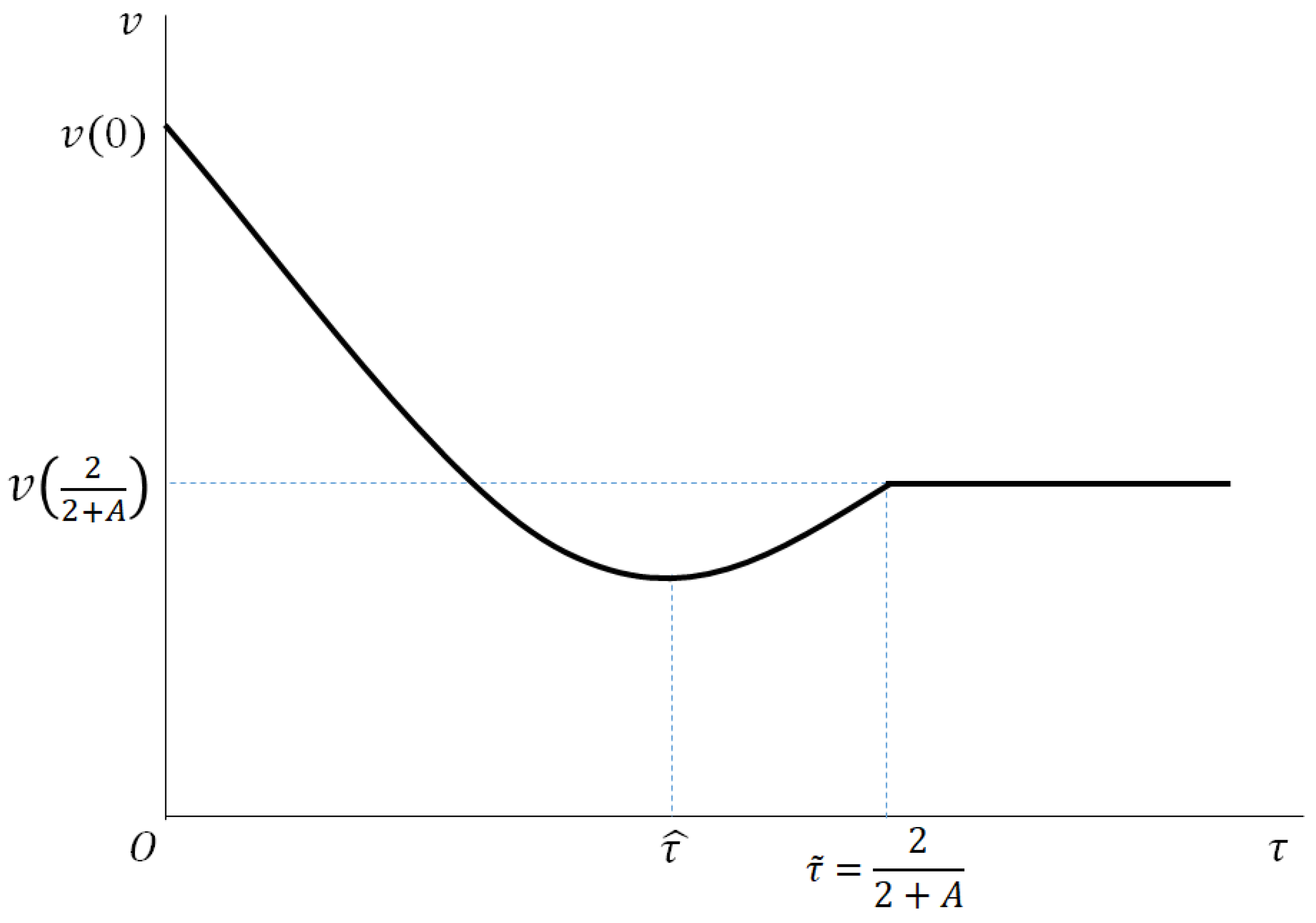
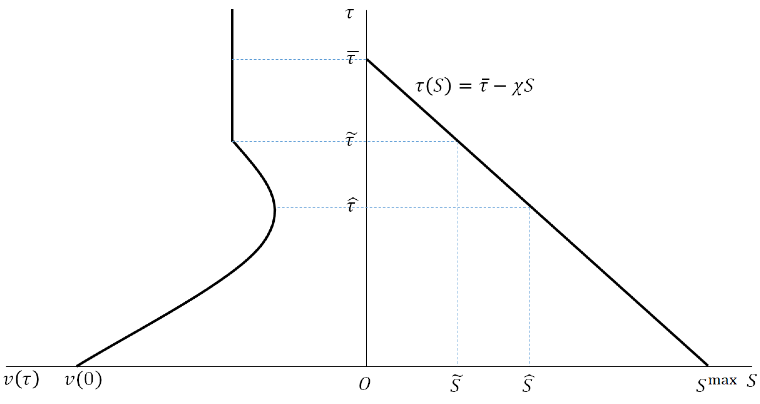
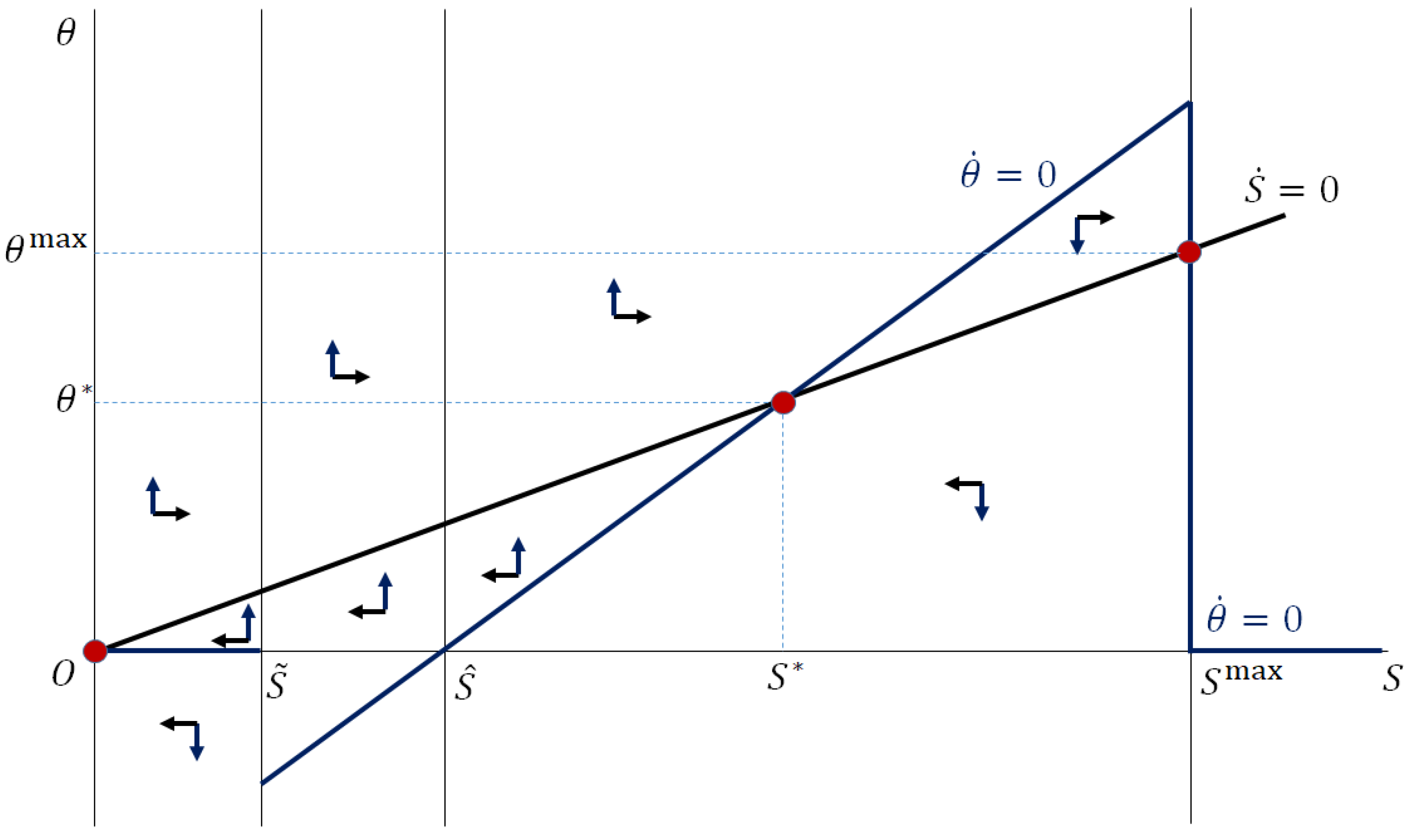
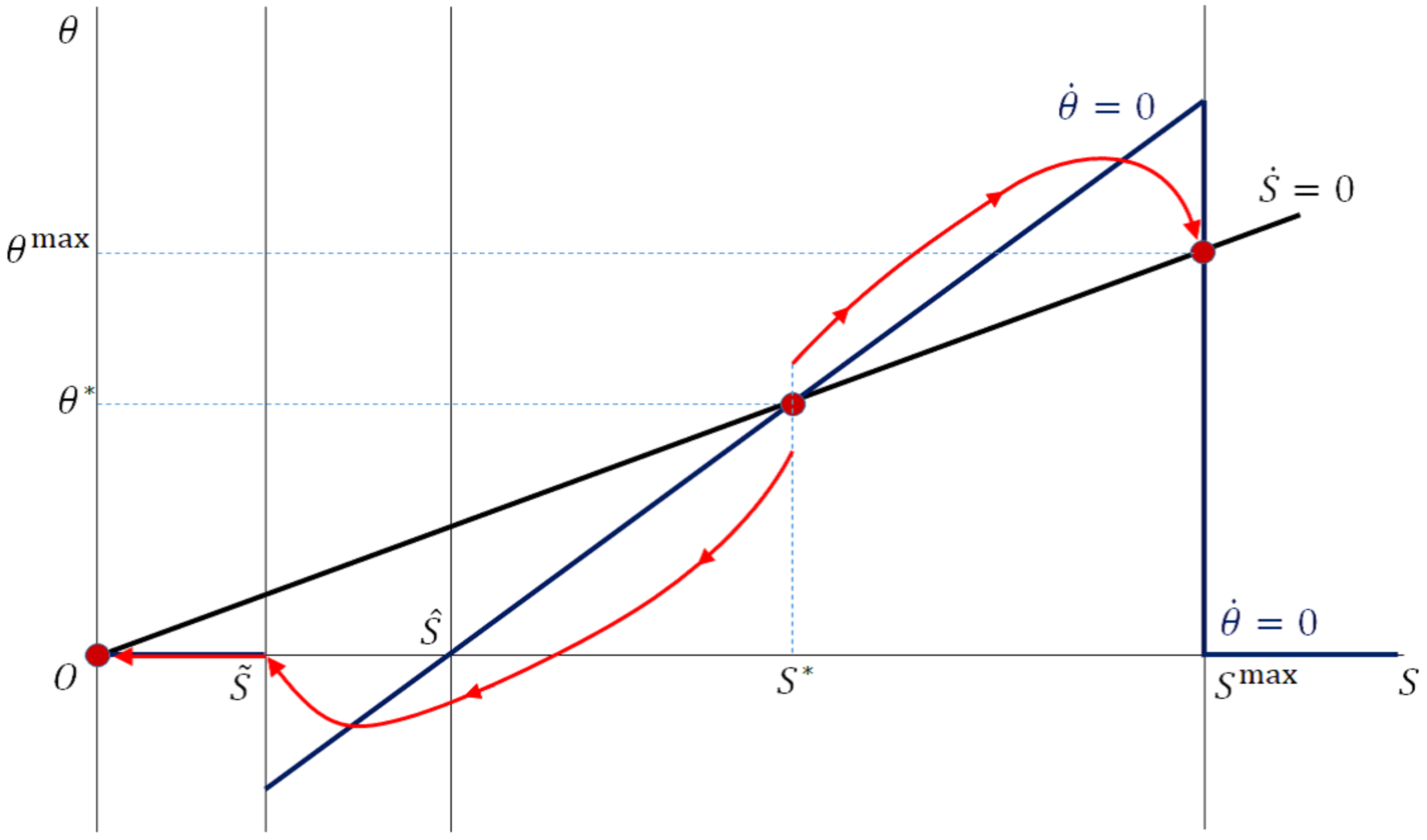
In this subsection, we characterize the open-loop Nash equilibrium of the policy game between symmetric countries by using a phase diagram in the $(S,\theta )$ plane.

4.1.1. The $\dot{\theta }=0$ Locus

Let us define “Region I” in the $(S,\theta )$ plane as the region such that $S\in \left[0,\tilde{S}\right]$. Since $\tau \ge \tilde{\tau }$ in Region I, we have $v^{\prime }\left(\tau \left(S\right)\right)=0$, and thus, (18) can be rewritten as $\dot{\theta }=(\rho +\delta )\theta$. Therefore, the $\dot{\theta }=0$ locus is the line $\theta =0$. Above this line, we have $\dot{\theta }>0$, and below this line, we have $\dot{\theta }<0$.

Consider next “Region II”, defined as the region such that $S\in \left(\tilde{S},\widehat{S}\right)$. In this region, we have $\widehat{\tau }<\tau <\tilde{\tau }$, and thus, $v^{\prime }\left(\tau \right)=b\tau -a>b\widehat{\tau }-a>0$. Thus, in Region II, $\dot{\theta }=(\rho +\delta )\theta +(1-\gamma )\chi \left[b(\overline{\tau }-\chi S)-a\right]$, and $\dot{\theta }=0$ iff $\theta =-(1-\gamma )\chi \left[b(\overline{\tau }-\chi S)-a\right]/(\rho +\delta )<0$. Therefore, the $\dot{\theta }=0$ locus in this region is given by the straight-line segment, with $\theta <0$ and with a positive slope ${\chi }^2(1-\gamma )b/(\rho +\delta )>0$. Above this line, we have $\dot{\theta }>0$, and below this line, we have $\dot{\theta }<0$.

Now, consider “Region III”, defined as the region such that $S\in \left[\widehat{S},S^{max}\right)$. In this region, we have $0<\tau <\widehat{\tau }$, and thus, $v^{\prime }\left(\tau \right)=b\tau -a<0$. Therefore, the locus $\dot{\theta }=0$ in Region III is given by the straight-line segment, with $\theta >0$ and with a positive slope ${\chi }^2(1-\gamma )b/(\rho +\delta )>0$. Above this line, we have $\dot{\theta }>0$, and below this line, we have $\dot{\theta }<0$.

Finally, consider “Region IV”, defined as the region with $S\ge S^{max}$. In this region, $\tau =0$ identically, and thus, $V^{\prime }\left(S\right)=-\chi v^{\prime }\left(\tau \left(S\right)\right)=0$. Then, we have $\dot{\theta }=(\rho +\delta )\theta$, and thus, the locus $\dot{\theta }=0$ is the line $\theta =0$.

To sum up, we obtain the following adjoint equation along the symmetric open-loop Nash equilibrium path:

$$\dot{\theta }=\left\{\begin{array}{cc}(\rho +\delta )\theta \hfill & \mathrm{for}0\le S\le \tilde{S},\hfill \\ (\rho +\delta )\theta +(1-\gamma )\chi \left[b(\overline{\tau }-\chi S)-a\right]\hfill & \mathrm{for}\tilde{S}<S<S^{max},\hfill \\ (\rho +\delta )\theta \hfill & \mathrm{for}S\ge S^{max}.\hfill \end{array}\right.$$

(23)

Note that at $S=S^{max}$, $v\left(\tau \right(S\left)\right)$ is not differentiable since ${lim}_{S\downarrow S^{max}}{v}^{\prime }\left(\tau \left(S\right)\right)=0$ and ${lim}_{S\uparrow S^{max}}{v}^{\prime }\left(\tau \left(S\right)\right)=a$. In this case, $\dot{\theta }=0$ implies that $\theta$ can take any value between zero and $(1-\gamma )\chi a/(\rho +\delta )$. With this fact and (23), we obtain the $\dot{\theta }=0$ locus as follows:

$$\theta =\left\{\begin{array}{cc}0\hfill & \mathrm{for}0\le S\le \tilde{S},\hfill \\ -(1-\gamma )\chi \left(b\overline{\tau }-a-b\chi S\right)/(\rho +\delta )\hfill & \mathrm{for}\tilde{S}<S<S^{max},\hfill \\ \forall \theta \in \left[0,(1-\gamma )\chi a/(\rho +\delta )\right]\hfill & \mathrm{for}S=S^{max},\hfill \\ 0\hfill & \mathrm{for}S>S^{max}.\hfill \end{array}\right.$$

(24)

4.1.2. The $\dot{S}=0$ Locus

In Region I, under symmetry, (14) implies that $\dot{S}=0$ iff $k=(\delta /2)S$. In light of Assumption 2 and the first-order condition (17), this means that the locus $\dot{S}=0$ in the $(S,\theta )$ plane is a line segment:

$$\theta =\frac{\beta \delta }{2}S.$$

(25)

Above this line, we have $\dot{S}>0$, and below this line, we have $\dot{S}<0$.

In Regions II, III, and IV, the same argument applies.

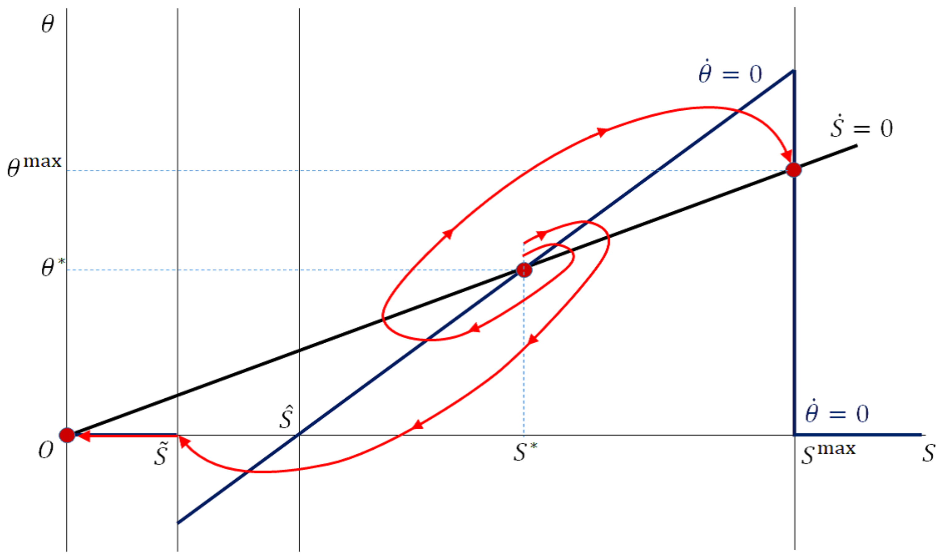
4.1.3. Steady States

A steady state is a point in which loci $\dot{\theta }=0$ given by (24) and $\dot{S}=0$ given by (25) intersect. In particular, if the line $\theta =(\beta \delta /2)S$ intersects the line $\theta =-(1-\gamma )\chi \left(b\overline{\tau }-a-b\chi S\right)/(\rho +\delta )$ at a point $S\in \left(\widehat{S},S^{max}\right)$, then that point is an interior steady state stock, which we denote by $S^{*}$. (The unique interior steady state comes from the assumption the cost function of the public investment is quadratic. If we assume instead that the cost function is given by $\beta k_i^{ϵ}/ϵ$, where $ϵ>2$, we may have multiple steady states.) A necessary condition for such an intersection is that the slope of the $\dot{S}=0$ locus is smaller than the slope of the $\dot{S}=0$ locus (in Regions II and III):

$$\frac{\beta \delta }{2}<\frac{(1-\gamma ){\chi }^{2}b}{\rho +\delta }.$$

(26)

However, (26) is not sufficient to ensure that $S^{*}$ in Region III. At $S=S^{max}$, the $\dot{S}=0$ locus satisfies $\theta =(\beta \delta /2)S^{max}$, and the $\dot{\theta }=0$ locus in Region III hits the point:

$$\theta =-\frac{(1-\gamma )\chi (b\overline{\tau }-a)}{\rho +\delta }+\frac{(1-\gamma ){\chi }^{2}b}{\rho +\delta }{S}^{max}.$$

Note that at $S=\widehat{S}$, the $\dot{S}=0$ locus satisfies $\theta =(\beta \delta /2)\widehat{S}>0$, and the $\dot{\theta }=0$ locus satisfies $\theta =0$. Therefore, if:

$$\frac{\beta \delta }{2}{S}^{max}<-\frac{(1-\gamma )\chi (b\overline{\tau }-a)}{\rho +\delta }+\frac{(1-\gamma ){\chi }^{2}b}{\rho +\delta }{S}^{max}$$

is satisfied, we have $S^{*}\in \left(\widehat{S},S^{max}\right)$. Since $S^{max}=\overline{\tau }/\chi$, the above condition can be rewritten as:

$$\frac{\beta \delta }{2}<\frac{(1-\gamma ){\chi }^{2}a}{(\rho +\delta )\overline{\tau }}.$$

(27)

Note that since $\widehat{\tau }=a/b<\overline{\tau }$ and, thus, $(1-\gamma ){\chi }^{2}a/\left[(\rho +\delta )\overline{\tau }\right]<(1-\gamma ){\chi }^{2}b/(\rho +\delta )$, (26) is always satisfied if the parameters satisfy (27).

Assumption 2. 

$$\frac{\beta \delta }{2}<\frac{(1-\gamma ){\chi }^{2}a}{(\rho +\delta )\overline{\tau }}.$$

We are now in a position to characterize the interior steady state, the property of which is described by the following proposition.

Proposition 2. 

There exists an interior steady state that achieves the stock of international infrastructure $S^{*}\in \left(0,S^{max}\right)$. This steady state is an unstable node (a spiral source) if:

$$\frac{{(\rho +2\delta )}^2}{4}>(<)\frac{2(1-\gamma ){\chi }^{2}b}{\beta }.$$

(28)

Proof. 

The existence of the interior steady state is obvious from Figure 4. To analyze stability, let us denote the value for $\theta$ at the interior steady state by ${\theta }^{*}$ and present a linearized dynamic system around the steady state $(S^{*},{\theta }^{*})$:

$$\left[\begin{array}{c}\dot{\theta }\\ \dot{S}\end{array}\right]=\left[\begin{array}{cc}\rho +\delta & -(1-\gamma ){\chi }^{2}b\\ 2/\beta & -\delta \end{array}\right]\left[\begin{array}{c}\theta -{\theta }^{*}\\ S-S^{*}\end{array}\right].$$

(29)

The determinant of the Jacobian matrix is:

$$\Delta \equiv \left|\begin{array}{cc}\rho +\delta & -(1-\gamma ){\chi }^{2}b\\ 2/\beta & -\delta \end{array}\right|=-(\rho +\delta )\delta +\frac{2(1-\gamma ){\chi }^{2}b}{\beta },$$

the sign of which is, in light of (26), positive. Since the trace of the Jacobian matrix is $\rho >0$, the two eigenvalues of the system must have positive real parts, and thus, the interior steady state is locally unstable. Moreover, the characteristic roots of the system (29) are $\left(\rho +\sqrt{{\rho }^2-4\Delta }\right)/2$ and $\left(\rho -\sqrt{{\rho }^2-4\Delta }\right)/2$. Thus, if ${\rho }^2-4\Delta >0$ ($<0$), which is equivalent to (28), the two characteristic roots are real (complex), and thus, the interior steady state is an unstable node (a spiral source). (Note that since ${(\rho +2\delta )}^2/4-(\rho +\delta )\delta ={\rho }^2/4>0$, ${(\rho +2\delta )}^2/4>2(1-\gamma ){\chi }^{2}b/\beta$ can be consistent with Assumption 2). □

In addition to the interior steady state $(S^{*},{\theta }^{*})$, there are two corner steady state solutions: one is $(S,\theta )=(0,0)$, in which the stock of international infrastructure is zero and there is no trade between two countries, and the other is $(S,\theta )=(S^{max},{\theta }^{max})$, in which there is two way trade in differentiated goods with zero trade costs.

Lemma 2. 

There exists a unique trajectory in the space $(S,\theta )$ that locally converges to the corner steady state $(S^{max},{\theta }^{max})$.

Proof. 

Consider any initial stock $S_0=S^{max}-ϵ$ for some small positive $ϵ>0$. Then, there is a continuum of associated possible values ${\theta }_0$ such that:

$$\overline{\theta }\left(S_0\right)\equiv \frac{\beta {\delta }^2}{4}{\left(S_0\right)}^2\ge {\theta }_0\ge -\frac{(1-\gamma )\chi (b\overline{\tau }-a)}{\rho +\delta }+\frac{(1-\gamma ){\chi }^{2}b}{\rho +\delta }{S}_0\equiv \underline{\theta }\left(S_0\right).$$

(30)

The trajectory that passes through the point $(S_0,{\theta }_0)$ has a negative slope at that point, given by:

$$\frac{d\theta }{dS}=\frac{d\theta /dt}{dS/dt}=\frac{(\rho +\delta ){\theta }_0+(1-\gamma )\chi \left[b(\overline{\tau }-\chi S_0)-a\right]}{2\sqrt{{\theta }_0/\beta }-\delta S_0}=\frac{(-)}{(+)}<0.$$

In light of (30), this slope is zero if $\theta =\overline{\theta }\left(S_0\right)$ and is minus infinity if ${\theta }_0=\underline{\theta }\left(S_0\right)$. For ${\theta }_0\in (\underline{\theta }\left(S_0\right),\overline{\theta }\left(S_0\right))$, the closer ${\theta }_0$ is to the upper value $\overline{\theta }\left(S_0\right)$, the flatter the slope is. Therefore, for given $S_0$, there exists exactly one corresponding ${\theta }_0$ such that the trajectory passing through $(S_0,{\theta }_0)$ leads to the steady state $(S^{max},{\theta }^{max})$. □

Thus, we can say that the steady state $(S^{max},{\theta }^{max})$ is “locally stable in the saddle-point sense” for $S_0$ located in some left-hand neighborhood of $S^{max}$ (i.e., for $S_0\in (S^{max}-ϵ,S^{max})$ for some small $ϵ>0$).

Lemma 3. 

For any $S_0\in \left(0,\tilde{S}\right)$, there is only one trajectory that leads to the trivial steady state $(0,0)$, and along that trajectory, it holds that $\theta \left(t\right)=0$ for all t.

Proof. 

If we associate $S_0\in \left(0,\tilde{S}\right)$ with some ${\theta }_0>0$, the trajectory passing through $(S_0,{\theta }_0)$ will move the system in the northeast direction, making S grow over time. Similarly, if we associate $S_0\in \left(0,\tilde{S}\right)$ with some ${\theta }_0<0$, the trajectory passing through $(S_0,{\theta }_0)$ will move the system in the southwest direction, making $\theta$ more and more negative as t increases. □

Thus, we can say that the steady state $(S,\theta )=(0,0)$ is also “locally stable in the saddle-point sense” for $S_0$ located in some right-hand neighborhood of zero (i.e., for $S_0\in (0,ϵ)$ for some small $ϵ>0$).

Note that the stability properties presented in Lemmas 2 and 3 are those in the neighborhood of the steady states. Although the analysis of global dynamics would be possible by solving the model numerically, Proposition 2 suggests some interesting possibilities.

Suppose that the interior steady state is an unstable node. Then, there can exist dynamic paths as illustrated in Figure 5. That is, if the initial stock of international infrastructure $S_0$ is below $S^{*}$, the world economy will converge to the steady state with a zero stock of infrastructure and no trade (i.e., the origin), and if $S_0$ is above $S^{*}$, the world economy will converge to the steady state with a maximum stock of infrastructure $S=S^{max}$ and zero trade cost. (It is easily verified that the Hamiltonian is not concave in S. This means that the open-loop Nash equilibrium path is not continuous at $S^{*}$. Therefore, the two paths moving towards the corner steady states generally do not pass the unstable steady state point $(S^{*},{\theta }^{*})$.) That is, whether the world economy achieves free trade and the highest welfare is history dependent.

Proposition 3. 

Suppose that ${(\rho +2\delta )}^2/4>2(1-\gamma ){\chi }^{2}b/\beta$ is satisfied in addition to Assumptions 1 and 2. If the initial stock $S_0$ is smaller (larger) than $S^{*}$, there can exist a dynamic path along which the infrastructure stock decreases (increases) over time, and the world economy would end up in autarky (free trade) in the long run.

In the presence of multiple long run equilibria in a dynamic model, which equilibrium is actually chosen is a crucial problem. Krugman [32] used a simple dynamic model with external economies and adjustment costs to examine whether initial conditions (i.e., “history”) determine the long run outcome or self-fulfilling prophecy (i.e., “expectations”) matters. In his model, history will dominate expectations if individuals’ discount rate is sufficiently large; intuitively, if the future is heavily discounted, individuals will not care much about the future actions of other individuals, and this will eliminate the possibility of self-fulfilling prophecies. Our finding, demonstrated in the condition in Proposition 3, is consistent with Krugman’s [32].

If the interior steady state is a spiral source, dynamic equilibria toward the steady state can be shown as in Figure 6. Krugman [32] discussed the case in which over some range, expectations rather than history are decisive and referred to the range of state variables from which either long run equilibrium can be reached as the “overlap”, and Fukao and Benabou [34] gave a precise characterization of the overlap. If there is an overlap and if the initial state is inside it, the economy’s equilibrium dynamics display indeterminacy, and self-fulfilling expectations can determine the long run outcome.

As mentioned earlier, the Hamiltonian is not concave in S. This means that the saddle-point path satisfies the necessary conditions for the optimality of each player, but not the sufficient conditions. This property generates another type of complexity that there may exist a “Skiba point” (Skiba [35]) $S^{\#}\ne S^{*}$ such that if $S_0<S^{\#}$, then the player’s optimal policy is to drive S to zero, while if $S_0>S^{\#}$, then his/her optimal policy is to build up S so that eventually $S^{max}$ is reached. The Skiba point generally differs from the unstable steady state stock $S^{*}$ if the unstable steady state $(S^{*},{\theta }^{*})$ is a spiral source. If a Skiba point exists, the dynamic equilibrium is again history-dependent; the initial stock of the infrastructure determines whether the world economy achieves a high level of the infrastructure stock that facilitates international trade. In order to find a Skiba point, we need to solve for the value functions corresponding to the stable steady states and find the point at which the two value functions intersect. As discussed by Deissenberg et al. [36], due to the lack of an appropriate “local” equation to define Skiba points, these points have to be determined numerically, and this is left for further research.

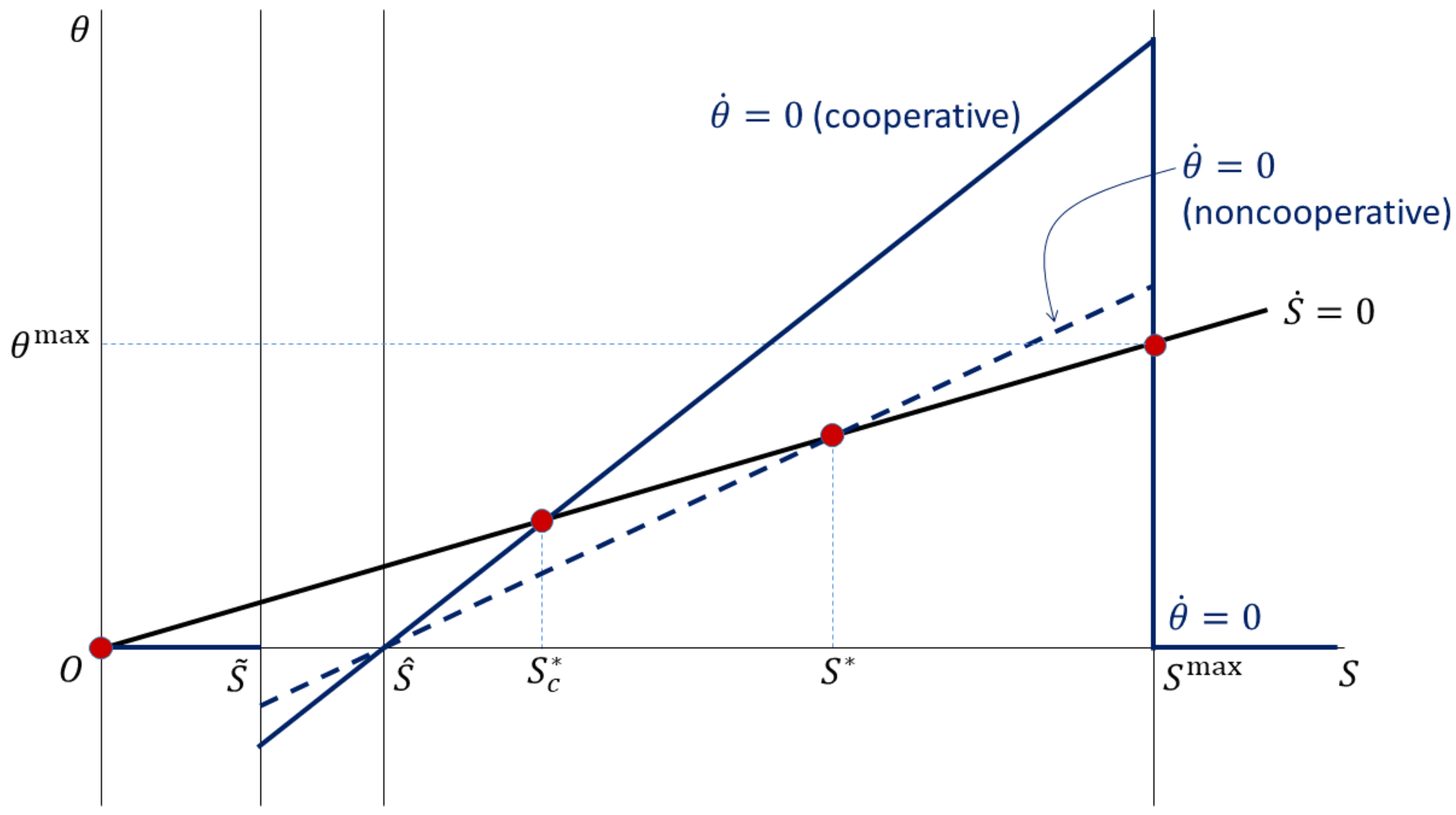
4.2. Comparison with the Cooperative Solution

Suppose that home and foreign governments cooperatively determine the public investment so as to maximize the joint welfare,

$${\int }_0^{\infty }{e}^{-\rho t}\left\{(1-\gamma )\left[v_H\left(\tau \left(S\left(t\right)\right)\right)+v_F\left(\tau \left(S\left(t\right)\right)\right)\right]+2-2f+2{\overline{q}}_0-\frac{\beta }{2}{k}_H{\left(t\right)}^2-\frac{\beta }{2}{k}_F{\left(t\right)}^2\right\}dt,$$

(31)

subject to (14). In this subsection, we derive the solution of this dynamic optimization problem under international cooperation and compare the open-loop Nash equilibrium to discuss the benefits of cooperative behavior.

The current-value Hamiltonian is defined as follows:

$$H=(1-\gamma )\left[v_H\left(\tau \left(S\right)\right)+v_F\left(\tau \left(S\right)\right)\right]-\frac{\beta }{2}{k}_H^2-\frac{\beta }{2}{k}_F^2+\theta \left(k_H+k_F-\delta S\right).$$

The first-order condition for optimal investment and the transversality conditions correspond to (17) and (19), respectively. The adjoint equation is now:

$$\dot{\theta }=\rho \theta -\frac{\partial H}{\partial S}=(\rho +\delta )\theta +(1-\gamma )\chi \left[v_H^{\prime }\left(\tau \left(S\right)\right)+v_F^{\prime }\left(\tau \left(S\right)\right)\right].$$

(32)

Since the two countries are assumed to be symmetric, we have the same critical values for $\tau$, that is $\tilde{\tau }\equiv 2/(2+A)$ and $\widehat{\tau }\equiv a/b$ defined in (22). The corresponding critical values for S are also the same as those in the noncooperative dynamic game. Investigating (32) in the regions between these critical values, we obtain the $\dot{\theta }=0$ locus as follows:

$$\theta =\left\{\begin{array}{cc}0\hfill & \mathrm{for}0\le S\le \tilde{S},\hfill \\ -2(1-\gamma )\chi \left(b\overline{\tau }-a-b\chi S\right)/(\rho +\delta )\hfill & \mathrm{for}\tilde{S}<S<S^{max},\hfill \\ \forall \theta \in \left[0,2(1-\gamma )\chi a/(\rho +\delta )\right]\hfill & \mathrm{for}S=S^{max},\hfill \\ 0\hfill & \mathrm{for}S>S^{max}.\hfill \end{array}\right.$$

(33)

The slope of the $\dot{\theta }=0$ locus in the cooperative solution in $\left(\tilde{S},S^{max}\right)$ is twice the slope of the $\dot{\theta }=0$ locus in the open-loop Nash equilibrium given by (24).

The $\dot{S}=0$ locus is given by (25), the same as that in the noncooperative equilibrium. Thus, the steady state solutions for the infrastructure stock and its shadow price are determined by (25) and (33). If Assumption 2 is satisfied and so is (26), it is clear that there is an interior cooperative solution in $\left(\tilde{S},S^{max}\right)$, as illustrated in Figure 7. Let us denote the infrastructure stock at this interior steady state by $S_c^{*}$. By examining the linearized dynamic system around the interior steady state, we can verify that this steady state is locally unstable. In addition to this unstable steady state, there are two steady states, one that achieves $S=0$ and the other that achieves $S=S^{max}$, and as in the case of noncooperative equilibrium, it can be verified that both steady states are local saddle points.

Since the steady state stock levels under the open-loop Nash equilibrium and cooperative solutions are respectively derived as:

$$S^{*}=\frac{2(1-\gamma )\chi (b\overline{\tau }-a)}{2(1-\gamma )b{\chi }^2-\beta \delta (\rho +\delta )}\mathrm{and}{S}_c^{*}=\frac{4(1-\gamma )\chi (b\overline{\tau }-a)}{4(1-\gamma )b{\chi }^2-\beta \delta (\rho +\delta )}$$

and thus,

$$\frac{S^{*}}{S_c^{*}}=\frac{4(1-\gamma )b{\chi }^2-\beta \delta (\rho +\delta )}{4(1-\gamma )b{\chi }^2-2\beta \delta (\rho +\delta )}>1,$$

we have $S_c^{*}<S^{*}$.

The linearized dynamic system around the interior steady state $(S_c^{*},{\theta }_c^{*})$ is:

$$\left[\begin{array}{c}\dot{\theta }\\ \dot{S}\end{array}\right]=\left[\begin{array}{cc}\rho +\delta & -2(1-\gamma ){\chi }^{2}b\\ 2/\beta & -\delta \end{array}\right]\left[\begin{array}{c}\theta -{\theta }_c^{*}\\ S-S_c^{*}\end{array}\right]$$

(34)

and thus, the interior steady state is an unstable node if ${\rho }^2-4{\Delta }_c>0$, where:

$${\Delta }_c\equiv \frac{4(1-\gamma )b{\chi }^2}{\beta }-(\rho +\delta )\delta .$$

Since ${\Delta }_c>\Delta >0$ if (26) is satisfied, the interior steady state in the open-loop Nash equilibrium is also an unstable node if ${\rho }^2-4{\Delta }_c>0$, or equivalently,

$${\rho }^2>4\left[\frac{4(1-\gamma )b{\chi }^2}{\beta }-(\rho +\delta )\delta \right].$$

(35)

Hence, the following proposition can be established.

Proposition 4. 

Suppose that (35) is satisfied in addition to Assumptions 1 and 2.

(i) If $S_0<S_c^{*}$, both the open-loop Nash equilibrium and the cooperative solution result in zero stock of infrastructure and, hence, autarky in the long run.

(ii) If $S_0\in \left(S_c^{*},S^{*}\right)$, the world economy would converge to the autarkic steady state with zero stock of infrastructure in the noncooperative equilibrium, whereas it can converge to the free trade steady state with $S=S^{max}$ in the presence of international cooperation.

(iii) If $S_0>S^{*}$, both the open-loop Nash equilibrium and the cooperative solution converge to the free trade steady state with the stock of infrastructure $S^{max}$.

We assume that the stock of infrastructure is an international public good, and thus, the lack of international cooperation tends to result in under-provision of the public good. Indeed, studies on the dynamic voluntary provision of public goods have shown that cooperative behavior leads to a higher steady state stock of infrastructure in comparison with noncooperative Nash equilibrium (e.g., Fershtman and Nitzan [28]). However, in the present framework of the model, the maximum steady state level of the infrastructure stock is $S^{max}$, irrespective of whether the countries cooperate or not. Therefore, there is no disadvantage of a lack of cooperation in the conventional sense if the initial stock of the infrastructure is sufficiently small or sufficiently large, as demonstrated in (i) and (iii) of Proposition 4. Nevertheless, international cooperation can be beneficial if the initial stock of infrastructure is at the moderate level, as demonstrated in Proposition 4 (ii). See also Figure 8, in which the initial stock $S_0$ is in $[S_c^{*},S^{*}]$. In this case, the open-loop Nash equilibrium results in zero stock of infrastructure, and thus, the world economy results in autarky, whereas international cooperation achieves the maximum level of the infrastructure stock and, thus, free trade. As demonstrated in Proposition 1, the cooperative solution achieves higher steady state welfare than the Nash equilibrium does. In other words, under international cooperation, the world economy can escape from a “low development trap” that would be caused by the noncooperative behavior of infrastructure investment.

5. Concluding Remarks

In this paper, we analyze a dynamic game of public infrastructure investment for reducing international trade costs in a two country world economy. We found that, depending on the trade costs and international distribution of manufacturing firms, the market equilibrium outcome is either two way intra-industry trade, one way inter-industry trade, or autarky. The national welfare in each country is affected by these trade patterns, and it is shown that in the presence of trade costs, free trade is not always beneficial relative to autarky. Because of the non-monotonic relationship between trade costs and national welfare, the dynamic equilibrium of the policy game turns out to generate the possibility of complex dynamics in the process of infrastructure accumulation. Specifically, we showed that the dynamic equilibrium of the policy game may exhibit history dependency in the sense that the initial stock of international infrastructure determines the subsequent dynamic path of the world economy including the pattern of international trade. We also compared the noncooperative equilibrium solution with an optimal solution under international cooperation on infrastructure investment and showed that the cooperative policy making may enable the world economy to escape from a “low development trap”.

Our analysis of the complex dynamics of noncooperative equilibrium is closely related to the existence of a Skiba point, which is analytically difficult to identify. This is because of the lack of an appropriate local equation to define Skiba points. We may find the Skiba point by solving the model numerically. In addition, our analysis focused on the open-loop Nash equilibrium, and it is interesting to show how the Markov-perfect Nash equilibrium of this policy game will look. Moreover, we focus on the case of symmetric countries and firms with identical production technologies. Even if we maintain the assumption of homogeneous firms, allowing for asymmetric countries leads to an analysis that needs numerical studies. Furthermore, in the case of asymmetric countries, there can be room for international transfer or taking over the investment by one of the countries. These are left for future research.

References

1. Anderson, J.E.; van Wincoop, E. Trade costs. J. Econ. Lit. 2004, 42, 691–751. [Google Scholar] [CrossRef]
2. Arvis, J.-F.; Duval, Y.; Shepherd, B.; Utoktham, C.; Raj, A. Trade Costs in the Developing World: 1996–2010. World Trade Rev. 2016, 15, 451–474. [Google Scholar] [CrossRef] [Green Version]
3. Jacks, D.S.; Meissner, C.M.; Novy, D. Trade Booms, Trade Busts, and Trade Costs. J. Int. Econ. 2011, 83, 185–201. [Google Scholar] [CrossRef] [Green Version]
4. Donaldson, D. Railroads of the Raj: Estimating the Impact of Transportation Infrastructure. Am. Econ. Rev. 2018, 108, 899–934. [Google Scholar] [CrossRef] [Green Version]
5. Allen, T.; Arkolakis, C. Trade and the Topography of the Spatial Economy. Q. J. Econ. 2014, 129, 1085–1140. [Google Scholar] [CrossRef] [Green Version]
6. Felbermayr, G.J.; Tarasov, A. Trade and the Spatial Distribution of Transport Infrastructure, CESifo Working Paper Series No. 5634. 2015. Available online: https://ideas.repec.org/p/ces/ceswps/_5634.html (accessed on 29 December 2020).
7. Bond, E.W. Transportation Infrastructure Investments And Trade Liberalization. Jpn. Econ. Rev. 2006, 57, 483–500. [Google Scholar] [CrossRef]
8. Hochman, G.; Tabakis, C.; Zilberman, D. The Impact of International Trade on Institutions and Infrastructure. J. Comp. Econ. 2013, 41, 126–140. [Google Scholar] [CrossRef]
9. Martin, P.; Rogers, C. Industrial Location and Public Infrastructure. J. Int. Econ. 1995, 39, 335–351. [Google Scholar] [CrossRef]
10. Mun, S.; Nakagawa, S. Pricing and Investment of Cross-border Transport Infrastructure. Reg. Sci. Urban Econ. 2010, 40, 228–240. [Google Scholar] [CrossRef] [Green Version]
11. Tsubuku, M. Endogenous Transport Costs and Firm Agglomeration in New Trade Theory. Pap. Reg. Sci. 2016, 95, 353–362. [Google Scholar] [CrossRef]
12. Anderson, J.A.; Marcouiller, D. Insecurity and the Pattern of Trade: An Empirical Investigation. Rev. Econ. Stat. 2002, 84, 342–352. [Google Scholar] [CrossRef] [Green Version]
13. Francois, J.; Manchin, M. Institutions, Infrastructure, and Trade. World Dev. 2013, 46, 165–175. [Google Scholar] [CrossRef] [Green Version]
14. Freund, C.L.; Weinhold, D. The Effect of the Internet on International Trade. J. Int. Econ. 2004, 62, 171–189. [Google Scholar] [CrossRef] [Green Version]
15. Limão, N.; Venables, A.J. Infrastructure, Geographical Disadvantage, Transport Costs and Trade. World Bank Econ. Rev. 2001, 15, 451–479. [Google Scholar] [CrossRef]
16. Allen, T.; Arkolakis, C. The Welfare Effects of Transportation Infrastructure Improvements. Unpublished manuscript. Available online: https://ideas.repec.org/p/nbr/nberwo/25487.html (accessed on 29 December 2020).
17. Bougheas, S.; Demetriades, P.O.; Morgenroth, E.L.W. Infrastructure, Transport Costs and Trade. J. Int. Econ. 1999, 47, 169–189. [Google Scholar] [CrossRef]
18. Bougheas, S.; Demetriades, P.O.; Morgenroth, E.L.W. International aspects of public infrastructure investment. Can. J. Econ. 2003, 36, 884–910. [Google Scholar] [CrossRef] [Green Version]
19. Brancaccio, G.; Kalouptsidiy, M.; Papageorgiouz, T. Geography, Search Frictions and Endogenous Trade Costs, NBER Working Paper No. 23581. 2017. Available online: https://econpapers.repec.org/paper/nbrnberwo/23581.htm (accessed on 29 December 2020).
20. Fajgelbaum, P.D.; Schaal, E. Optimal Transport Networks in Spatial Equilibrium, NBER Working Paper No. 23200. 2017. [Google Scholar]
21. McMillan, J. A Dynamic Analysis of Public Intermediate Goods Supply in Open Economy. Int. Econ. Rev. 1978, 19, 665–678. [Google Scholar] [CrossRef]
22. Bougheas, S.; Demetriades, P.O.; Mamuneas, T.P. Infrastructure, Specialization, and Economic Growth. Can. J. Econ. 2000, 33, 506–522. [Google Scholar] [CrossRef]
23. Yanase, A.; Tawada, M. History-Dependent Paths and Trade Gains in a Small Open Economy with a Public Intermediate Good. Int. Econ. Rev. 2012, 53, 303–314. [Google Scholar] [CrossRef]
24. Yanase, A.; Tawada, M. Public Infrastructure for Production and International Trade in a Small Open Economy: A Dynamic Analysis. J. Econ. 2017, 121, 51–73. [Google Scholar] [CrossRef]
25. Yanase, A.; Tawada, M. Public Infrastructure and Trade in a Dynamic Two-country Model. Rev. Int. Econ. 2020, 28, 447–465. [Google Scholar] [CrossRef]
26. Colombo, L.; Lambertini, L.; Mantovani, A. Endogenous transportation technology in a Cournot Differential Game with Intraindustry Trade. Jpn. World Econ. 2009, 21, 133–139. [Google Scholar] [CrossRef] [Green Version]
27. Devereux, M.B.; Mansoorian, A. International Fiscal Policy Coordination and Economic Growth. Int. Econ. Rev. 1992, 33, 249–268. [Google Scholar] [CrossRef]
28. Fershtman, C.; Nitzan, S. Dynamic Voluntary Provision of Public Goods. Eur. Econ. Rev. 1991, 35, 1057–1067. [Google Scholar] [CrossRef]
29. Figuières, C.; Prieur, F.; Tisball, M. Public Infrastructure, Non-cooperative Investments, and Endogenous Growth. Can. J. Econ. 2013, 46, 587–610. [Google Scholar] [CrossRef] [Green Version]
30. Han, Y.; Pieretti, P.; Zanaj, S.; Zou, B. Asymmetric Competition among Nation States: A Differential Game Approach. J. Public Econ. 2014, 119, 71–79. [Google Scholar] [CrossRef] [Green Version]
31. Itaya, J.-I.; Shimomura, K. A Dynamic Conjectural Variations Model in the Private Provision of Public Goods: A Differential Game Approach. J. Public Econ. 2001, 81, 153–172. [Google Scholar] [CrossRef]
32. Krugman, P. History versus Expectations. Q. J. Econ. 1991, 106, 651–667. [Google Scholar] [CrossRef]
33. Matsuyama, K. Increasing Returns, Industrialization, and Indeterminacy of Equilibrium. Q. J. Econ. 1991, 106, 617–650. [Google Scholar] [CrossRef] [Green Version]
34. Fukao, K.; Benabou, R. History versus Expectations: A Comment. Q. J. Econ. 1993, 108, 535–542. [Google Scholar] [CrossRef]
35. Skiba, A.K. Optimal Growth with a Convex-concave Production Function. Econometrica 1978, 46, 527–539. [Google Scholar] [CrossRef]
36. Deissenberg, C.; Feichtinger, G.; Semmler, W.; Wirl, F. Multiple Equilibria, History Dependence, and Global Dynamics in Intertemporal Optimization Models. In Economic Complexity (International Symposia in Economic Theory and Econometrics); Barnett, W.A., Deissenberger, C., Feichtinger, G., Eds.; Emerald Group Publishing: Bingley, UK, 2004; Volume 14, pp. 91–122. [Google Scholar]
37. Hartl, R.F.; Kort, P.M.; Feichtinger, G.; Wirl, F. Multiple Equilibria and Thresholds Due to Relative Investment Costs. J. Optim. Theory Appl. 2004, 123, 49–82. [Google Scholar] [CrossRef]
38. Oyama, D. History versus Expectations in Economic Geography Reconsidered. J. Econ. Dyn. Control 2009, 33, 394–408. [Google Scholar] [CrossRef] [Green Version]
39. Wagener, F.O.O. Skiba Points and Heteroclinic Bifurcations, with Applications to the Shallow Lake System. J. Econ. Dyn. Control 2003, 27, 1533–1561. [Google Scholar] [CrossRef]
40. Wirl, F. Indeterminacy and History Dependence of Strategically Interacting Players. Econ. Lett. 2016, 145, 19–24. [Google Scholar] [CrossRef]
41. Ottaviano, G.I.P.; Tabuchi, T.; Thisse, J.-F. Agglomeration and Trade Revisited. Int. Econ. Rev. 2002, 43, 409–436. [Google Scholar] [CrossRef]
42. Furusawa, T.; Konishi, H. Free Trade Networks. J. Int. Econ. 2007, 72, 310–335. [Google Scholar] [CrossRef] [Green Version]
43. Zhelobodko, E.; Kokovin, S.; Parenti, M.; Thisse, J.-F. Monopolistic Competition: Beyond the Constant Elasticity of Substitution. Econometrica 2012, 80, 2765–2784. [Google Scholar]
44. Brander, J.; Krugman, P. A ‘Reciprocal Dumping’ Model of International Trade. J. Int. Econ. 1983, 15, 313–321. [Google Scholar] [CrossRef] [Green Version]
45. Friberg, R.; Ganslandt, M. Reciprocal Dumping with Product Differentiation. Rev. Int. Econ. 2008, 16, 942–954. [Google Scholar] [CrossRef]
46. Fujiwara, K. Trade Liberalization in a Differentiated Duopoly Reconsidered. Res. Econ. 2009, 63, 165–171. [Google Scholar] [CrossRef]
47. Gilbert, J.; Oladi, R. International Trade and Welfare with Differentiated Goods and Strategic Asymmetry, Mimeo. Available online: http://www.etsg.org/ETSG2018/papers/006.pdf (accessed on 29 December 2020).
48. Yanase, A.; Long, N.V. Trade Costs and Strategic Investment in Infrastructure in a Dynamic Global Economy with Symmetric Countries, CIRANO Working Papers 2020s-59. 2020. Available online: https://ideas.repec.org/p/ces/ceswps/_8707.html (accessed on 29 December 2020).
Figure 1. Possible trade patterns.
Mathematics 09 00063 g001
Figure 2. Graph of v ( τ ) .
Mathematics 09 00063 g002
Figure 3. Threshold levels of τ and S.
Mathematics 09 00063 g003
Figure 4. Steady states in the symmetric open-loop Nash equilibrium.
Mathematics 09 00063 g004
Figure 5. History-dependent dynamics.
Mathematics 09 00063 g005
Figure 6. Indeterminacy of equilibrium paths.
Mathematics 09 00063 g006
Figure 7. Comparison of steady states between noncooperative and cooperative solutions.
Mathematics 09 00063 g007
Figure 8. Comparison of steady states between noncooperative and cooperative solutions.
Mathematics 09 00063 g008
Publisher’s Note: MDPI stays neutral with regard to jurisdictional claims in published maps and institutional affiliations.