Abstract
A radial basis function-finite differencing (RBF-FD) scheme was applied to the initial value problem of the Benjamin–Ono equation. The Benjamin–Ono equation has traveling wave solutions with algebraic decay and a nonlocal pseudo-differential operator, the Hilbert transform. When posed on , the former makes Fourier collocation a poor discretization choice; the latter is challenging for any local method. We develop an RBF-FD approximation of the Hilbert transform, and discuss the challenges of implementing this and other pseudo-differential operators on unstructured grids. Numerical examples, simulation costs, convergence rates, and generalizations of this method are all discussed.
1. Introduction
In this paper we use the benjamin–ono equation as a test-bed for new radial basis function-finite differencing (RBF-FD) simulations of nonlocal wave equations on non-uniform grids. The Benjamin–Ono equation presents the numerical challenges of numerical stiffness, a nonlocal pseudo-differential operator, and localized traveling solutions with slow decay. The equation
in which is the Hilbert transform, has many known exact solutions. For example, on , Equation (1) supports traveling solitary waves solutions:
The Benjamin–Ono equation is known to be well-posed [1] and integrable. It can be solved with inverse scattering, and many exact solution profiles are known [2,3]. It has been numerically simulated many times, both in the periodic setting [4] and on [5,6].
In this work we develop an RBF-FD scheme for the Benjamin–Ono equation. Common practice for the simulation of (1) on is to use periodic boundary conditions, allowing for Fourier collocation, on a large spatial domain [7]. Global radial basis functions (RBFs) have been used as a basis set for simulation of Benjamin–Ono [8]; instead, this work is the first example of the application of RBF-FD to this model. In many cases, RBFs allow for high orders of accuracy while taking advantage of non-uniform spacing in the node set when approximating linear operators. There are an increasing number of texts discussing the use of RBFs in the approximation of differential operators (see, e.g., [9,10]) while presenting much of their history and theory in detail. Recently, the concept of RBF-FD has been further extended to the approximation of definite integrals—first over smooth surfaces [11,12,13] and then over the volume of the ball [14]. In this paper we look at an extension of RBF-FD now to pseudo-differential operators. The method presented in this paper utilizes as a basis for approximation the so-called polyharmonic spline RBF augmented by shifted monomials. In this case, reference [15] explains that if the shifted monomials up to degree m are included in the basis for approximation, then all of the terms in the Taylor series up to degree m will be handled exactly for the function being interpolated. Therefore, for functions with rapidly decaying terms in the Taylor series, the linear operator will be applied to an approximation with accuracy on a node set with step size .
RBF-FD simulation of the Benjamin–Ono equation presents the challenge of creating a local approximation of a non-local pseudo-differential operator—the Hilbert transform. The process used herein is generalizable to other pseudo-differential operators, but is the primary cost of the method as it requires diagonalization of an RBF-FD differentiation matrix. Further, the spectrum of the RBF-FD differentiation matrix, particularly when constructed on non-uniform spaced node sets, can often include spurious eigenvalues (for example, with a positive, real part when approximating an operator with pure imaginary spectrum), similar to those observed in [16,17]. We observe that these spurious eigenvalues are the result of floating point errors due to the conditioning of the RBF-FD discretization of the linear operators.
Another complication is the slow decay of the solution as increases. To deal with this complication and with a localized steep gradient in the solutions, we increase the point density where the wave amplitude is large and decrease point density in the far field. This allows for increased accuracy over uniform grids with the same number of nodes. Consideration of non-uniform node sets is a key advantage of RBF based approximations. Even in the context of approximating a non-local operator with local approximations and slowly decaying solutions, we demonstrate accuracy where is the smallest spacing between adjacent points in a node set. We report errors based on this smallest step size, rather than the largest or the number of nodes as in [18,19], because the mapping we use to refine the node set both decreases the step size near important features of the solution and increases the large step sizes elsewhere while keeping the total number of nodes fixed. To further illustrate this method, we present a brief example in another model equation [20].
In the process of simulating the Benjamin–Ono equation, we present a simple framework for using RBF-FD to approximate pseudo-differential operators. The procedure extends the applicability of RBF methods beyond the purely differential equations previously simulated (see [16,21]) to a host of other pseudo-differential model equations—e.g., Whitham [22], Akers-Milewksi [20], and many more [23,24,25]. Many of these pseudo-differential equations exhibit coherent structures which are computed with quasi-Newton iteration [26,27]. The simulation of the dynamics near these coherent structures is the application where we believe this method will be most useful. The diagonalization cost required to approximate the pseudo-differential operators in our simulations (a pre-processing step) is comparable to the cost of the quasi-Newton iteration already being done to compute these waves [28].
The paper is organized as follows. Section 2 describes the RBF-FD based numerical method for simulating the Benjamin–Ono equation. This includes a discussion of RBF-FD, a node placement strategy, the approximation of a pseudo-differential operator, and the time-stepping scheme. Then, Section 3 presents numerical results when applying the method to both the Benjamin–Ono equation and the Akers–Milewski equation. Finally, Section 4 draws some conclusions about the use of these methods for approximation pseudo-differential operators.
2. Numerical Method
The numerical method begins in the familiar way of partitioning an interval using N subintervals. The endpoints of these subintervals are the sets of points . In this paper periodic boundary conditions on a large domain are imposed as a proxy for the slow decay of the solution as . To implement these boundary conditions, the method creates two periodic images of the set . These are defined by , where the signs each define a separate set and L is the period. Considering a point , define to be the set of n points in nearest to . The proposed method approximates the application of a linear operator to by interpolating u over the points in and then applying the linear operator to the interpolant. Traditional finite difference methods are defined in this way, where a polynomial interpolant of degree is constructed over the set and prescribed neighbors, and the linear operator is applied to the interpolant. The method proposed here, however, utilizes local RBF interpolation. RBF interpolation has been used successfully in the approximation of differential operators over subsets of scattered data through the concept of RBF-FD in, for instance, [10,29,30,31].
2.1. RBF-FD Weight Calculations for Linear Operators
For the simplicity of discussion, consider approximating applied to u at a point . That is, consider
Following common RBF/RBF-FD procedures, the interpolant is constructed via
with being function dependent only on the distance from the point . Note that the shift in the monomial terms is included for numerical stability when inverting the matrix in what follows. The interpolation coefficients , , and , , are chosen to satisfy the interpolation conditions , , along with constraints , for . By applying to the interpolant and then evaluating at , we wish to reduce the desired approximation to
A simple derivation can be carried out to show that the weights can be found by solving the system of linear equations . This system of equations includes the matrix
where and , for and ([10], Section 5.1.4). The right-hand side is the length column vector
The system of linear equations is uniquely solvable in our present context ([32], Theorem 8.21) and the weights , are the first n entries of the solution vector .
It is typical to approximate the action of on u at each point in simultaneously through the product , where D is an matrix and
The entries of D are found row by row (something that is easily parallelized), so that
that is, entry i of row k is nonzero only if (one of the points in ) or one of its periodic images, , appears in the set of the points nearest .
2.2. Node Placement
To construct node sets With non-uniform spacing that take advantage of the features of the solution, we first create a spatial node set with equal spacing on the domain . We then apply a nonlinear transformation:
The parameter a dictates the variation in step size in this transformation. For , the node set has uniform spacing; for the transformation degenerates by making the step size near the origin equal to zero. The transformation in Equation (3) is designed to preserve the overall domain length. It is by no means the only transformation which places a larger density of points near the origin and fewer far from the origin. We also ran experiments with the generalization
for . Increasing either p or a causes increased node density near the origin; however, it also leads to issues with the spectrum of the approximation of the linear operators, as we discuss in next section. For the numerical results presented in this work, we used only (3); examples of step-sizes for a sampling of a values in Equation (3) are in Figure 1.
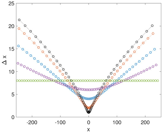
Figure 1.
The step sizes from (3) as a function of x. The horizontal equi-spaced case is . The step size becomes increasing variable as a ascends through the samples and (the extreme graph). The step size near the origin vanishes as . The domain has length , with points.
2.3. Approximating the Hilbert Transform
In this work we use degree seven polyharmonic splines as the radial basis functions, complemented with polynomials as described above, so that
These are a common choice for RBF-FD [10], but make the computation of pseudo-differential operators such as the Hilbert transform less straightforward than some other RBFs [8]. The classic procedure to approximate a linear operator using RBFs includes a step where the linear operator is exactly applied to the basis function. This has been done in a previous RBF-based numerical study of the Benjamin–Ono equation using gaussian basis functions on which the Hilbert transform can be exactly calculated [8]. For polyharmonic splines, an exact formula for the Hilbert transform is unavailable. Instead, we use ideas motivated by the Fourier transform definition of the Hilbert transform:
The Fourier transform definition reveals a relationship between the spectrum of the derivative operator, , and the spectrum of the Hilbert transform , so that
Using this relationship, if the spectrum of the derivative operator is known, then the spectrum of the Hilbert transform can be computed by an algebraic transformation of the spectrum of the derivative. We use this transformation to compute an approximation to the Hilbert transform by first computing a matrix which approximates the derivative, as described in Section 2.1. Next we diagonalize this matrix using QR iteration to get its eigenvalues and eigenvectors. The Hilbert transform can then be approximated using the same eigenvectors and Equation (5) applied to the computed to get its eigenvalues. This computation of the Hilbert transform, a pre-processing step, costs flops, where N is the number of spatial points. The time-stepping portion of the RBF-FD method is flops per step, due to the full matrix that approximates the Hilbert transform. The resulting method however, allows for non-uniform point spacing, so that larger domains can be accurately simulated with a fixed number of points. We expect this method to be competitive only in cases where there are fine local features of interest and slow decay to a remote boundary, as in the Benjamin–Ono solitary wave on . We admit that the Benjamin–Ono equation has special properties, i.e., integrability, which make other simulation methods such as inverse scattering available [3]. The above algorithm makes no use of integrability, and thus can be trivially extended to other equations with pseudo-differential operators, such as the intermediate-long wave [25], Whitham [22], and Akers–Milewski equations [20].
2.4. Time Stepping
For the time evolution of the system of differential equations induced by the RBF-FD spatial discretization of (1), we use a second order IMEX method [33],
in which is the nonlinear term (explicitly treated) and is the linear term (implicitly treated). This method is sometimes called SBDF [33], or extrapolated GEAR [34]. The linear stability region for this scheme is exterior to an egg-shaped region in the right half plane; it is unconditionally stable for wave equations—such as the Benjamin–Ono equation—that have pure imaginary linear spectra. We chose this method over the competing IMEX scheme CNAB (Crank–Nicholson Adams–Bashforth) so that small, real perturbations of the pure imaginary spectrum do not leave the stability region (as is the case for the CNAB). As we will see later, floating point errors due to the condition number of the matrices involved in RBF-FD discretization of the linear operators can cause changes in the spectrum of the approximation of the linear operators involved. We chose (6) to be as robust as possible to such errors.
The method we used to approximate the linear operators begins with an eigenvalue calculation. As such, other numerical time steppers are available—for example, exponential time differencing (ETD) [35] and integrating factors (IF) [36]. Since the equation is nonlinear, after diagonalizing the linear part, both ETD and IF methods require full matrix multiplications to evaluate the nonlinearity at each time step. The IMEX method used here has the inversion of a full matrix (for the implicit linear term); however, this can be done as a pre-processing step, so it also has a cost which scales like a full matrix multiplication per time step (and thus is comparable with ETD or IF). We chose the IMEX scheme due to its unconditional stability, to ameliorate the stiffness of this equation in explicit time steppers and to be robust to perturbations of the spectrum off the imaginary axis. In future work we plan to explore other time steppers, including higher order IMEX methods with unbounded stability regions [33].
3. Results
In this section, the numerical method described herein is evaluated via a number of numerical tests. We show the effects of the numerical discretization and truncation error, and the effect of truncating to finite length. Errors are measured as a function the minimal step size of our non-uniform parameterization. The effect of the non-uniform step-size on the spectrum of approximation to the linear operator is also discussed. Example simulations of algebraically decaying Benjamin–Ono solitary waves are shown, along with an oscillatory exponentially decaying wave in the Akers–Milewski equation.
In Figure 2, we display an example of a simulation of the Benjamin–Ono solitary wave:
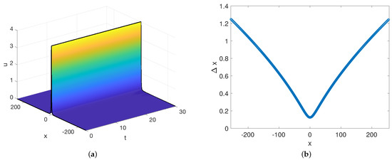
Figure 2.
(a) The soliton solution propagated on a domain . (b) The step-sizes used for the RBF-FD discretization used in the left simulation.
The simulation was computed in a frame which travels with the wave so that the wave appears stationary. As is common practice, a large domain size with periodic boundary conditions was used as a proxy for [7] since the solution decays as . The crest of the wave profile, in the left panel, is marked with a solid black line, to highlight the lack of oscillation in time. The initial profile is also marked with a solid black line for highlighting purposed. The right panel shows the step sizes used for this simulation, which range over an order of magnitude with . The node spacing is concentrated near the origin, where the wave (and its derivatives) is largest; the largest spacing occurs for large x, where the wave is small. This allows for increased accuracy for the same number of points as compared to uniform step sizes.
In Figure 3, we study the accuracy of the spatial discretization of the linear operator
when applied to the solitary wave (7). There are two competing parameters which determine the spatial accuracy, the domain size L, and the minimal space step . We present two experiments, one where the domain size is varied for a sampling of parameterizations (left panel of Figure 3) and one where the parameterization is varied for a fixed domain size (right panel of Figure 3). In the left panel, all discretizations show an initial decrease in error as the domain size increases, scaling like , up to a point where the truncation error of the discretization of the linear operator grows to be larger than the domain discretization error. For each discretization, including Fourier, there is a length L for which the method is most accurate (for a fixed number of points). All of the RBF-FD discretizations, based on (3), are able to give a more accurate discretization than a Fourier discretization (with the best observed improvement at ). That these methods outperform a Fourier discretization on the Benjamin–Ono solitary wave is natural, since a periodic tiling of this wave has a discontinuous first derivative at the boundary, limiting the accuracy of a Fourier discretization. The variable space step RBF-FD is not limited by this discontinuity, even with an approximation that assumes more than one continuous derivative at the boundary. The accuracy of the RBF-FD discretization of the linear operator as a function of minimal step size (controlled by the parameter a) is depicted in the right panel of Figure 3, in which we observe accuracy. Given that the approximation of the linear operator was formed by applying the linear operator to an interpolant with a basis set of polynomials terms up to degree eight and polyharmonic splines of , it is not surprising to see accuracy since the interpolation procedure provides for at least that order of accuracy [15].
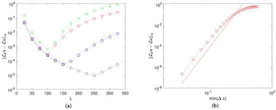
Figure 3.
The infinity norm of the error of the numerical approximation of the linear operator, , against the exact on the solitary wave is depicted. (a) The error’s dependence on domain size, L, is compared for the RBF-FD discretization using the spatial points in (3) with (red triangles), (blue circles), and (black squares), and an equi-spaced Fourier discretization (green stars). All of these computations use . (b) The error dependence on the minimal step size for , altering the step size with the parameter “a”. The numerical results are marked with triangles; the continuous line marks .
The method used here to discretize the linear operator in Equation (8) is based on a diagonalization of a RBF-FD differentiation matrix. First we compute an RBF-FD approximation of a derivative matrix. Next we compute the eigenvalues and eigenvectors of this matrix. As we knew the exact spectrum of the derivative and the Hilbert transform in the infinite dimensional problem from Fourier analysis,
we constructed eigenvalues of the discrete Hilbert transform by applying the same relationship to the discrete problem. If is an eigenvalue of the differentiation matrix, then the eigenvalues of the discretized Hilbert transform are defined to satisfy
Eigenvalue manipulation based on the above definition is used to find all the eigenvalues of the approximation to (8); the eigenvector matrix (and its inverse) of the RBF-FD differentiation matrix is then multiplied by diagonal matrices with this approximate spectrum to get an approximation for (8). Although the eigenvalues were constructed to be pure imaginary, as is the spectrum of the exact problem, the result of the matrix multiplication (by the matrix of eigenvectors and its inverse) can perturb the spectrum due to machine precision errors. These errors scale with the condition number of the matrix of the eigenvectors of the RBF-FD differentiation matrix. As is the case for classic polynomial interpolation, the condition number of this matrix grows as the points get closer together. This increase in condition number results in a corresponding increase in the size of spurious real eigenvalues of the discretized linear operator (which poses a stability problem for numerical time stepping algorithms). To observe this phenomenon, after creating the approximate linear operator , we apply a QR iteration to compute the eigenvalues of this matrix. That these computed eigenvalues differ at all from the desired spectrum is a direct result of the conditioning of the eigenspace of RBF-FD differentiation matrix. An example of the computed spectrum of the matrix used to evolve the Benjamin–Ono solitary wave in Figure 2 is in the left panel of Figure 4. This spectrum includes spurious eigenvalues with a real part as large as . In the right panel of Figure 4, we observe the dependence of the eigenvalue with the largest real part as a function of the parameter a from Equation (3). The match between the size of the eigenvalues and the condition number of the matrix of eigenvectors, F, times the machine precision, is displayed in the right panel of Figure 4.
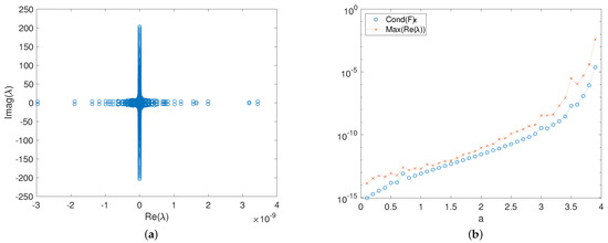
Figure 4.
(a) The spectrum of the linear operator used for the evolution depicted in Figure 2. (b) The condition number and the maximally real eigenvalue of the approximation of the linear operator as a function of the step-size parameter “a” in Equation (3), marked with xs, is compared to the condition number of eigenvector matrix, F, of the RBF-FD differentiation matrix times the machine precision, , marked with circles.
Examples of the discretized eigenfunctions are plotted in Figure 5. These eigenfunctions were all computed on a domain of length ; the panels each show different subsets of the computational domain. As the discretization becomes coarser near the boundary (), globally supported eigenfunctions are more poorly resolved. This is natural, as a trade-off for better resolution near the origin. The exact relationship between the resolution of the eigenfunctions and the errors in the argument of the corresponding eigenvalues is unknown. This does, however, point to a possible explanation for the ill-conditioning of the eigenspace of the differentiation matrix. Poor resolution of globally supported eigenfunctions could be the cause; the ill-conditioned eigenspace could be due to some points being too far apart, rather than too close together (as is typical in polynomial interpolation matrices).
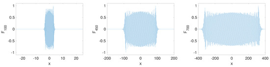
Figure 5.
The real part of three sample eigenfunctions is depicted. These eigenfunctions have eigenvalues with “spurious” real parts and respectively. These values were computed with , , and .
A few references have studied the behavior of eigenvalue stability with regard to node placement. This includes [16] which investigates special node distributions that improve eigenvalue stability for global RBF methods, and [37,38,39,40,41,42] which investigate the effects of using mapped nodal sets on the accuracy and eigenvalue stability of finite-difference and pseudo-spectral methods. These works may provide the framework for future research avenues which resolve the relationship between node placement the ill-conditioning of the eigenspace of differential operators.
The method presented here and error analysis are presented in the context of the Benjamin–Ono equation, where the combination of algebraic decay of the solitary wave and nonlocal nature of the Hilbert transform make a challenging testbed for a numerical scheme. The same ideas generalize easily to other nonlocal equations; it is trivial to apply this method to the Whitham equation [22] or the Akers–Milewski equation [20,43]. The Akers–Milewski equation,
supports traveling, wavepacket-type solitary waves [44]. These waves decay exponentially in space, and thus do not present the same challenges for numerical simulation, (Fourier collocation is spectrally accurate) as the Benjamin–Ono solitary wave (7). As evidence of the ease of generalizing this approach, we include an example of the evolution of such a wave using RBF-FD discretization a non-uniform grid in Figure 6.
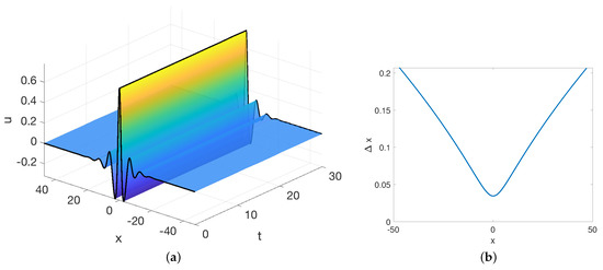
Figure 6.
(a) An example of the evolution of a traveling wavepacket-type solitary wave in the Akers–Milewski Equation (9). (b) The step sizes used for this simulation.
Although the method is presented in one spatial dimension with periodic boundary conditions, its application is not exclusive to either. The exact methodology can be directly applied for higher dimensional problems (for example, the two-dimensional solutions of Akers–Milewski [20]). In order to consider different boundary conditions, one needs a relationship between the spectrum of the derivative operator and that of the pseudo-differential operator with the new boundary conditions. This relationship may be simple to determine (for example, the relationship for homogeneous Dirichelet boundary conditions agreeing with that of the periodic case), in which case the definition of the pseudo-differential operator is unchanged and the boundary conditions may be implemented with standard RBF-FD methods. For general boundary conditions the relationship between the derivative’s spectra and the pseudo-differential operator’s spectra should be investigated before applying the method.
4. Conclusions
In this paper an RBF-FD implementation of the Benjamin–Ono equation was presented. This required the development of an RBF-FD implementation of the Hilbert transform. An approximation of the Hilbert transform was built by manipulating the spectrum of a differentiation matrix. This approach generalizes simply to other pseudo-differential operators, but incurs an pre-processing cost, meaning that this method is expensive compared to a Fourier implementation. The approach, however, allows for arbitrary boundary conditions and non-uniform grids. We expect it to be most useful in problems where an pre-processing cost is already being paid, for example, in the evolution of a coherent structure which was computed via quasi-Newton iteration. A future avenue for research is in the relationship between the node placement and the conditioning of the eigenspace of the differentiation matrix; we observe that this plays a key role in the accuracy of the approximation of the spectrum of the linear operator.
Author Contributions
Conceptualization, B.A.; methodology, B.A. and J.R.; software, B.A., J.R., and T.L.; validation, B.A., J.R., and T.L.; formal analysis, B.A., J.R., and T.L.; writing—original draft preparation, B.A., J.R., and T.L.; writing—review and editing, B.A., J.R., and T.L.; visualization, B.A.; supervision, B.A.; project administration, B.A.; funding acquisition, B.A. All authors have read and agreed to the published version of the manuscript.
Funding
This research received no external funding.
Acknowledgments
All three authors acknowledge the support of Office of Naval Research via the project Atmospheric Propagation Sciences for High Energy Lasers. B.F. Akers acknowledges support from the Air Force Office of Sponsored Research’s Computational Mathematics Program via the project Radial Basis Functions for Numerical Simulation.
Conflicts of Interest
This report was prepared as an account of work sponsored by an agency of the United States Government. Neither the United States Government nor any agency thereof, nor any of their employees, make any warranty, express or implied, or assume any legal liability or responsibility for the accuracy, completeness, or usefulness of any information, apparatus, product, or process disclosed, or represent that its use would not infringe privately owned rights. Reference herein to any specific commercial product, process, or service by trade name, trademark, manufacturer, or otherwise does not necessarily constitute or imply its endorsement, recommendation, or favoring by the United States Government or any agency thereof. The views and opinions of authors expressed herein do not necessarily state or reflect those of the United States Government or any agency thereof.
References
- Tao, T. Global well-posedness of the Benjamin–Ono equation in H1 (R). J. Hyperbolic Differ. Equat. 2004, 1, 27–49. [Google Scholar] [CrossRef]
- Matsuno, Y. Interaction of the Benjamin-Ono solitons. J. Phys. A Math. Gen. 1980, 13, 1519. [Google Scholar] [CrossRef]
- Kaup, D.; Matsuno, Y. The inverse scattering transform for the Benjamin–Ono equation. Stud. Appl. Math. 1998, 101, 73–98. [Google Scholar] [CrossRef]
- Ambrose, D.M.; Wilkening, J. Computation of time-periodic solutions of the Benjamin–Ono equation. J. Nonlinear Sci. 2010, 20, 277–308. [Google Scholar] [CrossRef][Green Version]
- Feng, B.F.; Kawahara, T. Temporal evolutions and stationary waves for dissipative Benjamin–Ono equation. Phys. D Nonlinear Phenom. 2000, 139, 301–318. [Google Scholar] [CrossRef]
- Pelloni, B.; Dougalis, V.A. Numerical solution of some nonlocal, nonlinear dispersive wave equations. J. Nonlinear Sci. 2000, 10, 1–22. [Google Scholar] [CrossRef]
- Kalisch, H. Error analysis of a spectral projection of the regularized Benjamin–Ono equation. BIT Numer. Math. 2005, 45, 69–89. [Google Scholar] [CrossRef][Green Version]
- Boyd, J.P.; Xu, Z. Comparison of three spectral methods for the Benjamin–Ono equation: Fourier pseudospectral, rational Christov functions and Gaussian radial basis functions. Wave Motion 2011, 48, 702–706. [Google Scholar] [CrossRef]
- Fasshauer, G.E. Meshfree Approximation Methods with MATLAB; World Scientific: Singapore, 2007; Volume 6. [Google Scholar]
- Fornberg, B.; Flyer, N. A Primer On Radial Basis Functions With Applications To The Geosciences; SIAM: Philadelphia, PA, USA, 2015. [Google Scholar]
- Reeger, J.A.; Fornberg, B. Numerical quadrature over the surface of a sphere. Stud. Appl. Math. 2016, 137, 174–188. [Google Scholar] [CrossRef]
- Reeger, J.A.; Fornberg, B.; Watts, M.L. Numerical quadrature over smooth, closed surfaces. Proc. R. Soc. A Math. Phys. Eng. Sci. 2016, 472. [Google Scholar] [CrossRef]
- Reeger, J.A.; Fornberg, B. Numerical quadrature over smooth surfaces with boundaries. J. Comput. Phys. 2018, 355, 176–190. [Google Scholar] [CrossRef]
- Reeger, J.A. Approximate Integrals Over the Volume of the Ball. J. Sci. Comput. 2020, 83. [Google Scholar] [CrossRef]
- Bayona, V. An insight into RBF-FD approximations augmented with polynomials. Comput. Math. Appl. 2019, 77, 2337–2353. [Google Scholar] [CrossRef]
- Platte, R.B.; Driscoll, T.A. Eigenvalue stability of radial basis function discretizations for time-dependent problems. Comput. Math. Appl. 2006, 51, 1251–1268. [Google Scholar] [CrossRef]
- Sarra, S.A. A numerical study of the accuracy and stability of symmetric and asymmetric RBF collocation methods for hyperbolic PDEs. Numer. Methods Part. Differ. Equ. Int. J. 2008, 24, 670–686. [Google Scholar] [CrossRef]
- Libre, N.A.; Emdadi, A.; Kansa, E.J.; Shekarchi, M.; Rahimian, M. A multiresolution prewavelet-based adaptive refinement scheme for RBF approximations of nearly singular problems. Eng. Anal. Bound. Elem. 2009, 33, 901–914. [Google Scholar] [CrossRef]
- Davydov, O.; Oanh, D.T. Adaptive meshless centres and RBF stencils for Poisson equation. J. Comput. Phys. 2011, 230, 287–304. [Google Scholar] [CrossRef]
- Akers, B.; Milewski, P.A. A model equation for wavepacket solitary waves arising from capillary-gravity flows. Stud. Appl. Math. 2009, 122, 249–274. [Google Scholar] [CrossRef]
- Shen, Q. A meshless method of lines for the numerical solution of KdV equation using radial basis functions. Eng. Anal. Bound. Elem. 2009, 33, 1171–1180. [Google Scholar] [CrossRef]
- Ehrnström, M.; Kalisch, H. Traveling waves for the Whitham equation. Differ. Integral Equat. 2009, 22, 1193–1210. [Google Scholar]
- Akers, B.; Milewski, P.A. Dynamics of three-dimensional gravity-capillary solitary waves in deep water. SIAM J. Appl. Math. 2010, 70, 2390–2408. [Google Scholar] [CrossRef]
- Akers, B.; Milewski, P.A. Model equations for gravity-capillary waves in deep water. Stud. Appl. Math. 2008, 121, 49–69. [Google Scholar] [CrossRef]
- Ablowitz, M.; Fokas, A.; Satsuma, J.; Segur, H. On the periodic intermediate long wave equation. J. Phys. A Math. Gen. 1982, 15, 781. [Google Scholar] [CrossRef]
- Parau, E.; Vanden-Broeck, J.M.; Cooker, M. Nonlinear three-dimensional gravity-capillary solitary waves. J. Fluid Mech. 2005, 536, 99–105. [Google Scholar] [CrossRef]
- Oliveras, K.; Curtis, C. Nonlinear travelling internal waves with piecewise-linear shear profiles. J. Fluid Mech. 2018, 856, 984–1013. [Google Scholar] [CrossRef]
- Claassen, K.M.; Johnson, M.A. Numerical bifurcation and spectral stability of wavetrains in bidirectional Whitham models. Stud. Appl. Math. 2018, 141, 205–246. [Google Scholar] [CrossRef]
- Flyer, N.; Lehto, E.; Blaise, S.; Wright, G.B.; St-Cyr, A. A Guide to RBF-generated finite-differences for nonlinear transport: Shallow water simulations on a sphere. J. Comput. Math. 2012, 231, 4078–4095. [Google Scholar] [CrossRef]
- Flyer, N.; Wright, G.; Fornberg, B. Radial Basis function-generated finite differences: A mesh-free method for computational geosciences. In Handbook of Geomathematics; Freeden, W., Nashed, M.Z., Sonar, T., Eds.; Springer: Berlin/Heidelberg, Germany, 2014. [Google Scholar] [CrossRef]
- Fornberg, B.; Flyer, N. Solving PDEs with radial basis functions. Acta Numer. 2015, 24, 215–258. [Google Scholar] [CrossRef]
- Wendland, H. Scattered Data Approximation; Cambridge University Press: Cambridge, UK, 2005. [Google Scholar]
- Ascher, U.; Ruuth, S.; Wetton, B. Implicit-explicit methods for time-dependent partial differential equations. SIAM J. Numer. Anal. 1995, 32, 797–823. [Google Scholar] [CrossRef]
- Varah, J.M. Stability restrictions on second order, three level finite difference schemes for parabolic equations. SIAM J. Numer. Anal. 1980, 17, 300–309. [Google Scholar] [CrossRef]
- Kassam, A.K.; Trefethen, L. Fourth-order time-stepping for stiff PDEs. SIAM J. Sci. Comput. 2005, 26, 1214–1233. [Google Scholar] [CrossRef]
- Milewski, P.; Tabak, E. A pseudospectral procedure for the solution of nonlinear wave equations with examples from free-surface flows. SIAM J. Sci. Comput. 1999, 21, 1102–1114. [Google Scholar] [CrossRef]
- Kosloff, D.; Tal-Ezer, H. A modified Chebyshev pseudospectral method with an O (N-1) time step restriction. J. Comput. Phys. 1993, 104, 457–469. [Google Scholar] [CrossRef]
- Bayliss, A.; Turkel, E. Mappings and accuracy for Chebyshev pseudo-spectral approximations. J. Comput. Phys. 1992, 101, 349–359. [Google Scholar] [CrossRef]
- Shen, J.; Wang, L.L. Error analysis for mapped Legendre spectral and pseudospectral methods. SIAM J. Numer. Anal. 2004, 42, 326–349. [Google Scholar] [CrossRef][Green Version]
- Zhong, X.; Tatineni, M. High-order non-uniform grid schemes for numerical simulation of hypersonic boundary-layer stability and transition. J. Comput. Phys. 2003, 190, 419–458. [Google Scholar] [CrossRef]
- Shukla, R.K.; Zhong, X. Derivation of high-order compact finite difference schemes for non-uniform grid using polynomial interpolation. J. Comput. Phys. 2005, 204, 404–429. [Google Scholar] [CrossRef]
- Orszag, S.A. Accurate solution of the Orr–Sommerfeld stability equation. J. Fluid Mech. 1971, 50, 689–703. [Google Scholar] [CrossRef]
- Diorio, J.; Cho, Y.; Duncan, J.H.; Akylas, T. Gravity-capillary lumps generated by a moving pressure source. Phys. Rev. Lett. 2009, 103, 214502. [Google Scholar] [CrossRef]
- Akers, B.F.; Seiders, M. Numerical Simulations of Overturned Traveling Waves. In Nonlinear Water Waves; Springer: Berlin/Heidelberg, Germany, 2019; pp. 109–122. [Google Scholar]


Publisher’s Note: MDPI stays neutral with regard to jurisdictional claims in published maps and institutional affiliations. |
© 2020 by the authors. Licensee MDPI, Basel, Switzerland. This article is an open access article distributed under the terms and conditions of the Creative Commons Attribution (CC BY) license (http://creativecommons.org/licenses/by/4.0/).