Abstract
A copula is a multivariate cumulative distribution function with marginal distributions . For this reason, a classical kernel estimator does not work and this estimator needs to be corrected at boundaries, which increases the difficulty of the estimation and, in practice, the bias boundary correction might not provide the desired improvement. A quantile transformation of marginals is a way to improve the classical kernel approach. This paper shows a Beta quantile transformation to be optimal and analyses a kernel estimator based on this transformation. Furthermore, the basic properties that allow the new estimator to be used for inference on extreme value copulas are tested. The results of a simulation study show how the new nonparametric estimator improves alternative kernel estimators of copulas. We illustrate our proposal with a financial risk data analysis.
1. Introduction
Based on the kernel method and transformations, we present a new nonparametric estimator of a multivariate copula that improves the empirical copula and the most prominent kernel estimators (see reference [], for a detailed review). We use the new estimator to analyse and test the extreme value dependence between the losses in the Spanish stock market index and different stock market indexes of Europe, USA and China.
The copula model allows us to represent the dependence structure of a multivariate random vector of continuous variables , which combines with marginal distributions to give the multivariate distribution. This idea was established in the fundamental theorem proposed by Sklar []. This theorem shows that a multivariate cumulative distribution function (cdf) H of the random vector , with marginal distributions functions , has associated a copula C, so that:
In practice, the dependence structure and marginal distributions are unknown and both will need to be fitted. We assume that marginal cdfs can be easily adjusted using parametric distributions or nonparametric methods and we focus on the fitting of dependence structure using a copula. It is often difficult by visualizing the data to select the appropriate dependency structure and, therefore, the right copula model. Alternatively, a nonparametric estimation of a copula can be obtained whose results can be used for estimating joint probabilities or for testing the adequacy of a copula family, for example, the extreme value copula family. In this paper, these two aims of our new nonparametric estimator are analysed through a simulation study.
Because there are a lot of dependence structures represented by different copulas families, specific tests for choosing the best copula are useful. The approach for developing a test for the adequacy of copulas takes its lead from, for example, the proposal of Genest and Rivest [] for bivariate Archimedean copulas; the test of Scaillet [] on inference for the positive quadrant dependence hypothesis; the test for equality between two copulas of [] or the test of symmetry for bivariate copulas of Genest et al. [].
On inference for extreme value copulas, alternative types of tests have been proposed, among which the most well known are the test of Genest et al. [] based on a Cramér-von Mises statistic, the test analysed by Ghorbal et al. [] based on an U-statistic and the test of Kojadinovic et al. [] that uses the - property and is also based on a Cramér-von Mises statistic (see also [] for complete properties of the test based on - property).
The test proposed by Kojadinovic et al. [] is based on the empirical copula that is equivalent to the multivariate empirical distribution. However, the empirical copula is inefficient for certain shapes of distribution, for example, when the marginal cdfs are associated with extreme value distributions. Alternatively, Omelka et al. [] analyse how testing extreme value copula can be based on different kernel estimators. The main difficulty of a classical kernel estimator is its bias on the boundaries when the function values at these points are positive. Based on this concern, Chen and Huang [] analyse the kernel copula estimator with local linear boundary correction which the authors proved reduces bias and variance. Alternatively, Omelka et al. [] propose the transformation of a kernel copula estimator based on standard normal inverse distribution function transformations, which is very easy to implement and has the same weak convergence properties as the previous proposal. In this paper, an improved transformed kernel estimator is proposed that has the same weak convergence properties and is useful for the inference on extreme value copulas. The theoretical results are shown for the bivariate case, but they are easily extrapolated to the multivariate case.
In Section 2, we present the background on kernel estimation of copulas, the new estimator and its theoretical asymptotic properties for testing the - property of extreme value copulas. Section 3 presents the simulation results that allow us to analyse finite-sample properties and inference errors type 1 and 2. As an illustration, in Section 4, a financial risk analysis is carried out where the extreme value copula family hypothesis between the Spanish stock market index and different neighbouring and non-neighbouring countries is tested. Finally, we conclude in Section 5.
2. Kernel Estimation of Copulas
Let , ∀, be a sample of n independent and identically distributed (i.i.d.) bivariate data, the product kernel estimator of the bivariate cdf can be expressed as:
where K is the cdf associated with the kernel function k, that is a bounded or asymptotically bounded and symmetric probability density function (pdf) (see [,] for a review on kernel estimation of the multivariate distribution function). Examples of such functions are the Epanechnikov and the Gaussian kernels (see []). The parameters and , known as the bandwidths or smoothing parameters, control the smoothness of the estimation. Thus, the larger the value of and , the smoother the resulting function. Their values depend on the sample size n—the biggest sample size n, the lower the smoothing parameters—but obtaining optimal values for these smoothing parameters is one of the greatest difficulties posed by the kernel estimation.
Based on Slark’s theorem, from (2) we specify the kernel estimator of copula as:
where , , are estimators of the marginal cdfs that, in practice, can be obtained based on a parametric distribution or with a non-parametric estimator. Given that the copulas allow us to separate dependence structure from marginal distribution, we focus on estimating the first; so, the aim is to estimate a multivariate cdf with marginal distributions, whose kernel estimator for bivariate case is expressed as:
where, unlike (2), given that the marginal distributions are , we assume and as , taking into account the relationship between b and n, hereinafter we denote it as . In practice, we need to define observations , ∀, the values of the marginal empirical distributions , and , are a natural choice. However, it is known that empirical distribution takes value 1 at the maximum value observed and most of the commonly used copulas (Gumbel, Clayton, Gaussian and Student’s t) are not finite derivatives (copula density values) at corners ; then, these empirical distributions are replaced by corrected versions that are known as pseudo-data and that can be defined as: or, as Chen and Huang [] suggested, . So, the kernel estimator of a copula is defined as:
To obtain the estimator defined in (5) a kernel function, K, needs to be selected that will have minimal effect on the results obtained, and to calculate the bandwidth , whose value will have an important effect on the estimated copula. The bandwidth can be calculated using some cross-validation or plug-in method or using the rule-of-thumb proposed by Silverman [] for the kernel estimator of pdf adapted to the kernel estimator of cdf (see [,]).
The properties of a kernel estimator depend on some smoothness characteristics of the cdf; in our context in particular, it is a requirement that the first two derivatives take finite values different from zero. Furthermore, when the distribution has a bounded domain and the density at boundary takes positive values, as in the case of the bivariate copula with domain on , the estimator defined in (5) has boundary bias. This means that the kernel estimator at boundary is not consistent (see [] pp. 46–47, for a clear description in the kernel density estimator context). This is problematic since our aim is to test if our data is generated by an extreme value copula. There are three alternative proposals to achieve consistency at boundary of a kernel estimator of a copula. Boundary kernel methods are the most common techniques proposed in the context of kernel regression and density estimation (see [,]), the main difficulty with the use of this type of kernel being that it does not integrate one which, in practice, could be inconvenient. Chen and Huang [] proposed a kernel estimator of copulas with linear boundary correction, the weakness of their method is that for many common families of copulas (e.g., Clayton, Gumbel, Gaussian and Student’s t) the bias at some of the corners of the unit square is only of order , versus the that is reached in the central values of the domain, where is the asymptotic order operator. Another way to correct boundary bias is using the mirror-reflection kernel estimator, this method being proposed by Gijbels and Mielniczuk [] to estimate the density of the copula. In all cases, the main difficulty of a kernel estimator with or without boundary bias is calculating the smoothing parameter whose value will greatly affect the results.
An alternative strategy to avoid boundary bias and to calculate the smoothing parameter easily is to transform marginal distributions of the copula so that the kernel estimator of the new marginal distributions does not have boundary bias and their shapes allow us to minimise the bias of the kernel estimator. This idea also addresses the problems of the estimator defined in (3) based on the original scale of the data. On the one hand, although the marginal distributions are not uniform, they can have shapes that could also be subject to inconsistency at the boundaries, i.e., the distribution could have bounded domain on one or both sides with positive density. On the other hand, the problems associated with the kernel estimator defined in (3) are widely known when the distribution to estimate has one or two long tails (see [,,]).
The transformed estimator of the copula is based on the equality:
i.e., the values of the copula function C evaluated on original scale are equal to the values of function evaluated on transformed scale. So, the transformed kernel estimator (TKE) of a copula is defined as:
where is a transformation which is equal to the inverse of a given continuous cdf. The estimator defined in (6) has a fundamental advantage over the kernel estimator defined in (5) and its versions that incorporate boundary bias reduction; given that the function is the inverse of a given cdf, we know the marginal distributions of and the bandwidth can be calculated based on these distributions.
Omelka et al. [] proposed that , where is the cdf of the standard normal distribution. This standard normal transformation is based on the idea that the normal distribution does not have boundary bias problems and it can be estimated easily using a classical kernel estimator. This transformed estimator is called Gaussian transformed kernel estimator and is defined as:
In practice, in this case the value of bandwidth can be calculated using the idea of rule-of-thumb of Silverman [] applied to the standard normal marginal cdfs, that is . In the simulation study presented in Section 3, we show the difference between the mean integrated squared error of a copula, , using optimal and using the proposed rule-of-thumb.
We propose an alternative estimator to the one defined in (7) using a transformation T that is better than . Our proposal is based on the second-order approximation properties of univariate kernel estimator of marginal distributions. When as , f is a continuous pdf and the first derivative exists, the bias and variance of kernel estimator of cdf are (see [,,]):
and
By addition of the integrated variance and the integrated squared bias, we can approximate the MISE of the kernel estimation of marginal distributions as:
where the integral limits are given by the domain of argument variable Y. From expression (10) it is easy to deduce that the distribution that minimises MISE also minimises the functional . Terrell [] found the pdf family that minimises the functionals of type , where p is the order of the derivative. This principle was applied to cdf and quantile kernel estimation by Alemany et al. [], who showed how the , whose pdf and cdf are:
minimises the functional , , and therefore minimises the integrated bias of the classical kernel estimator of a cdf. Section 2 includes the theoretical results on testing extreme value copulas, and Theorem 1 shows as the cdf M has the properties that allow us to conclude that the kernel estimator of does not have boundary bias (see []). So, the Beta transformed kernel estimator of a copula is:
where can be calculated using rule-of-thumb applied to the marginal distributions, that is . In the simulation study shown in Section 3, the MISE calculated with this bandwidth is compared to the one that minimises MISE.
Next, we present some theoretical results related to the weak convergence to a Gaussian process of the estimator defined in (12) and the - property for testing extreme value copulas.
Theoretical Results
We use the result from Fermanian et al. [] for the weak convergence of the kernel estimator of a copula defined in (5) to a Gaussian process in the space of all bounded real-valued functions on , i.e., , which is expressed as follows:
where , are the partial derivatives of the function C with respect to , ⟼ indicates weak convergence and is a Brownian bridge on with covariance function:
where ∧ is the minimum.
The weak convergence defined in (13) requires that the copula has continuous partial derivatives. Furthermore, Omelka et al. [] proved the weak convergence of local linear, mirror reflection and Gaussian transformed kernel estimators of copula. These authors remark that it is sufficient to assume that the first partial derivatives are continuous on , i.e., we can eliminate the corners. This is an important result, given that most of the commonly used copulas (Clayton, Gumbel, Normal and Student’s t) do not have finite partial derivatives at the corners.
The weak convergence of our Beta transformed kernel estimator is defined in the following theorem.
Theorem 1.
Let us suppose a continuous copula C, with continuous first order partial derivatives and bounded second order partial derivatives on that satisfies the following asymptotic properties: , and . If the Beta transformed kernel estimator meets the weak convergence defined in (13).
Proof of Theorem 1.
Let be the inverse transformation function in , the proof of Theorem 1 comes directly from the results of Theorem 2 in Omelka et al. [], who proved that, if the first derivative and are bounded, then converge weakly to the Gaussian process . For we have that , and , . Directly, we know that the pdf m of the is bounded. Moreover, if the quotient is analysed, the maximum is approximately found at . □
The weak convergence of Theorem 1 allows us to use for the inference on copulas. We focus on an extreme value copula test based on the proposal of Kojadinovic et al. [], that analyses the - property associated with this family of copulas (see, for example, []). A copula is - if and in the null hypothesis is not rejected from the alternative . In practice, we test the - hypothesis using some values of (see []),
To test the previous hypotheses we propose estimating = using the Beta transformed kernel estimator of the copula, i.e., .
Proposition 1.
If the partial derivatives of the copula are continuous then for any we have:
in .
Proof of Proposition 1.
The result in Proposition 1 is obtained from:
Using the convergence of Theorem 1:
We now need to prove the weak convergence of . To this end, we use the result of Kojadinovic et al. [], that proved the weak convergence of this difference for empirical copula (see also []). In general, this result can be directly extrapolated to the kernel estimator and, in particular, to the Beta transformed kernel estimator, considering that . Then, under , , it weakly converges to process (14). □
For hypothesis testing given a fixed r, we use a Cramér-von Mises statistic:
and for a range of values , the following statistic can be considered:
For implementing the test based on , we use the numerical approximation proposed by Kojadinovic et al. [], replacing the empirical copula by a Beta transformed kernel estimator of the copula. The procedure is as follows:
- The statistics are approximated using a uniformly spaced grid , , of points on , i.e., .
- R independent copies of , are generated, such thatwhere are independent copies of . The process of obtaining these independent copies of is described in Appendix A.
- To calculate the copies of as and to obtain the p-value of the statistics as:
3. Simulation Study
We summarise the results of our simulation study, we aim to evaluate the finite sample properties of our Beta transformed kernel estimator in (12), and compare it with the empirical copula, with the classical kernel estimator in (5) and with the Gaussian transformed kernel estimator in (7). We also obtain some results using boundary kernel, but the computational times are longer and in our simulation study we do not achieve better results than those obtained with classical kernel.
We show two types of results; in the former, the errors between the estimations and true copulas are compared and, in the latter, the differences between the extreme value copula tests obtained with the empirical copula and with the Beta transformed kernel estimator are analysed.
3.1. Analysing the Errors of Kernel Estimators
To carry out the study, we simulate 500 samples of size and from different family and parameters of copulas that are indicated in the tables with the simulation results shown in this section. The alternative estimators are compared approximating the using a grid uniformly spaced in points on . The Epanechnikov kernel is used in all cases. Furthermore, bandwidth needs to be calculated, its value has an important impact on the results. Sometimes, the calculation of requires long optimization processes based on leave-one out estimators (see [] for a review on kernel density estimation). Alternatively, the rule-of-thumb similar to the proposal of Silverman [] can be used; however, to calculate the rule-of-thumb smoothing parameter we would need to use a parametric copula with a given parameter. A direct alternative, based on the product kernel estimator, consists of using the rule-of-thumb based on independent marginal reference distribution. The difficulty with marginal is that , , and the rule-of-thumb smoothing parameter based on the proposal of Silverman [] can not be calculated. In this case, to use the standard normal bandwidth is an easy solution (see [] for an example on kernel density estimation of transformed data). In our simulation study, two types of results are shown, on the one hand, the obtained with the rule-of-thumb bandwidth based on standard normal distribution for kernel and Gaussian transformed kernel estimator and based on for Beta transformed kernel estimator. On the other hand, the obtained optimizing the approximate on a grid the values for .
To facilitate the interpretation of the results, we calculate the quotient between the MISE obtained for each kernel estimator and the one obtained using the empirical copula. The reference values of MISE for the empirical copula are shown in Table A1 in Appendix B. Table 1 and Table 2 contain, respectively, the quotients for the analysed elliptical and archimedean copulas. These results show how, using the adequate smoothing parameter, the analysed kernel estimators improve the empirical copula. Focusing on archimedean copulas in Table 1, it can be seen that, if the optimal smoothing parameter is used, in all cases the best results are obtained with the Beta transformed kernel estimator (). With the optimal bandwidth, the Gaussian transformed kernel estimator () only slightly improves the classical kernel estimator () for Gumbel with dependence parameter equal to 3 and 4, i.e., for the most extreme value dependence copulas. In Table 2, for elliptical copulas, the results with optimal smoothing parameter are similar, is the best and improves when the data is generated by the most extreme value copulas, the Student’s t with dependence parameter equal to .

Table 1.
Quotient betweenthe approximate MISE of kernel estimators of the copula (numerator) and approximate MISE of the empirical copula (denominator) for elliptical copulas (* indicates optimal bandwidth).
Table 2.
Quotient between the approximate MISE of kernel estimators of the copula (numerator) and approximate MISE of the empirical copula (denominator) for archimedean copulas (* indicates optimal bandwidth).
In practice, we will not know what the optimal smoothing parameter is, and having estimators that allow this parameter to be obtained in a direct and simple way is essential. As shown in Table 1 and Table 2, and have this characteristic; in both cases the results with the rule-of-thumb smoothing parameter are near the optimal results and the lowest MISEs are obtained with .
3.2. Test for Extreme Value Copula
We show the results of a reduced simulation study (to avoid long computing periods) that allows us to compare type 1 and 2 errors of the extreme value copula test on smaller-sized samples, calculated from the empirical copula (proposed by []) and from the Beta transformed kernel estimator () proposed in this paper, where the optimal bandwidth is used. For this experiment, we use 100 samples of size . Both tests are implemented using a uniformly spaced points on for calculating and with estimated copies of , . The results for type 1 errors are shown in Table 3 for theoretical extreme value copulas with which is true. Table 4 shows the type 2 errors for copulas with non-dependence in extreme. They indicate that using we reduce type 1 error at the cost of increasing type 2 error, although for this error is already high for the test based on the empirical copula. In general, a larger-size sample is required for reducing type 2 error.
Table 3.
Error type 1 calculated with different significant levels .
Table 4.
Error type 2 calculated with different significant levels .
The results in Table 3 imply that, if the data is generated by an extreme value copula, based test practically ensures a correct result. This is fundamental in the context of risk quantification, given that the consequences of not detecting extreme dependency could be more serious than those of not detecting the opposite, i.e., non-dependence in extreme.
4. Data Analysis
For illustrating the usefulness of our proposed estimator , we analyse the dependence between the Spanish stock market index (IBEX35) and the stock market indexes of some neighbouring European countries, namely Germany (DAX), France (CAC40), Italy (FTSE MIB), Portugal (PSI20) and United Kingdom (FTSE100) as well as the two principal stock market indexes of the USA (DOWJONES and S&P500) and the Hong Kong stock market index (HANG SENG) (see [] for an analysis of extreme dependence between markets).
Two types of results are shown:
- The fit of non parametric copulas to estimate the probability that the observed losses of two stock market indexes together exceed some percentiles, i.e., we estimate the value of , , with the analysed kernels estimators.
- The test to analyse if the data is generated by an extreme value copula.
To carry out the analysis we use a database of the monthly losses of the stock market indexes from January 2000 to March 2021. These losses are calculated from the quotes of the analysed indexes that are public and can be downloaded, for example, from Investing.com. Throughout the period analysed, three major events influenced market performance leading to higher losses than in periods of stability: the Lehman Brothers crisis that began in September 2008, the referendum on Brexit on 23 June 2016, and the ongoing COVID-19 crisis which started in March 2020. The three events are considered systemic risks that affect all markets and, if this effect is simultaneous, the data should be generated by an extreme value copula. In Table 5, the main descriptive statistics of the losses in percentage are shown. Furthermore, normality tests and a positive skewness test are carried out and, in all cases, normality hypothesis is rejected and skewness greater than zero can not be rejected, i.e., in absolute value, positive losses are bigger that negative ones.
Table 5.
Descriptive statistics of monthly losses in percentage: Means, Standard Deviation (STD), Minimum (Min), First Quantile (Q25), Median, Third Quantile (Q75), Maximum (Mas), Skewness and Kurtosis.
The losses of the Spanish stock market index are plotted together with the indexes of the countries listed for comparison. In Figure 1, we compare Spain (in blue) with four countries that also currently belong to the European Union (in black) and, Figure 2, the comparison is made with the other countries (in black).
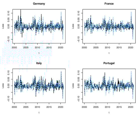
Figure 1.
Losses of Spanish stock market index (dashed line in blue) and stock market indexes of four countries in the European Union (solid line in black).
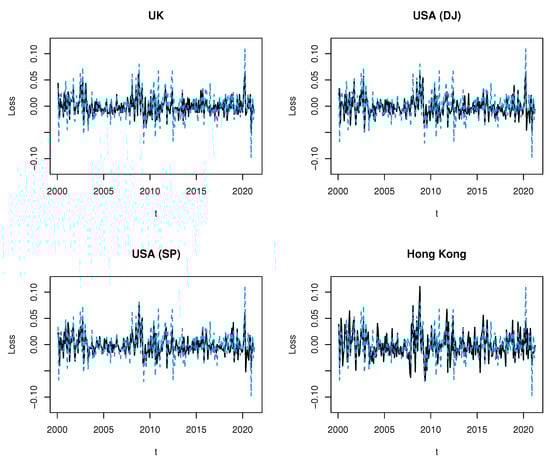
Figure 2.
Losses of Spanish stock market index (dashed line in blue) and stock market indexes of four countries outside of the European Union (solid line in black).
To obtain the Beta transformed kernel estimator we need the data to be i.i.d. so, with this in mind, we analyse if the the monthly losses of the stock market indexes have some kind of time dependence on the mean or on the variance. The simple and partial autocorrelation functions of the series and the square series allows us to find the model used to filter series and to get i.i.d. data (see, for example, []). The filter models used are shown in Table A2 of Appendix A.
In Table 6, we show the results of for estimated with , i.e., the probability of jointly exceeding a given extreme quantile. The upper tail dependence can be approximated as . In Appendix C, we show that the results obtained with the empirical copula and provide lower values than . It should be noted that the empirical copula tends to underestimate the probability of the tail when extreme values exist. Furthermore, in the simulation study improves for all the compared copulas.
Table 6.
Values of for Spain and the countries analysed.
We obtain the results of the extreme value copula test of Kojadinovic et al. [] based on the empirical copula, and the same test based on the Beta transformed kernel estimator that is analysed in this paper, using the asymptotically optimal smoothing parameter and a grid of 4 values around it. As expected, all the results indicate that all the analysed bivariate data have a dependence structure generated by an extreme value copula. This behaviour has been accentuated by the COVID-19 crisis, which has led to greater losses and a systemic risk that lasts over time (see [,] for a review on effect of COVID-19 on markets returns and volatility). In Figure 3 and Figure 4, pairs of pseudo-data are plotted; in all cases some accumulation of points is detected near the corner , which is an indicator of extreme value dependence.
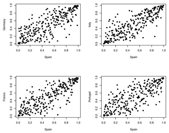
Figure 3.
Pseudo-data for each bivariate copula between Spain and Germany, Italy, France and Portugal.
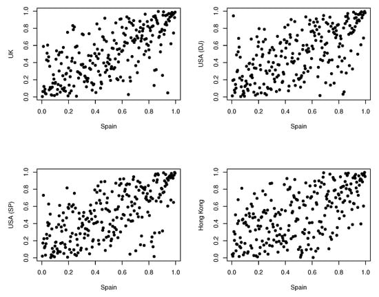
Figure 4.
Pseudo-data for each bivariate copula between Spain and UK, USA (DJ and SP) and Hong Kong.
5. Conclusions
A new kernel estimator of a copula based on a transformation is analysed. The asymptotic theoretical properties that allow it to be used for inference are proved. A simulation study shows that the proposed estimator improves the alternative estimator in the most common copulas.
The new estimator allows us to reduce the type 1 error associated with the extreme value copula test, while the type 2 error increases slightly. A future line of work would be to investigate how to reduce the type 2 error with a small sample size of the tests based on the - property.
The financial data analysis shows that the new estimator is useful for the risk analysis linked to the dependence between stock markets.
Author Contributions
Conceptualization, C.B. and C.A.A.; methodology, C.B.; software, C.A.A.; validation, C.B., C.A.A.; formal analysis, C.B.; investigation, C.A.A.; resources, C.B.; data curation, C.A.A.; writing—original draft preparation, C.B. and C.A.A.; writing—review and editing, C.B. and C.A.A.; visualization, C.B. and C.A.A.; supervision, C.B. All authors have read and agreed to the published version of the manuscript.
Funding
This research received no external funding
Data Availability Statement
Acknowledgments
The authors gratefully acknowledge support from the BBVA Foundation and the Spanish Ministry of Science and Innovation grant PID2019-105986GB-C21.
Conflicts of Interest
The authors declare no conflict of interest.
Appendix A. Procedure to Obtain Independent Copies
To generate independent copies of we use the result of Proposition 1 and under we define . Following Kojadinovic et al. [], replacing the empirical copula by a Beta transformed kernel estimator of copula, the Gaussian process is estimated as:
where is a large number of copies. In expression (A1) we have that , where are i.i.d. random variables with mean 0 and variance 1, so that , is the probability function. Finally, we obtain the copies of the statistic for the extreme value copula test as:
Appendix B. Simulation Study
Results of simulation study. Table A1 shows the MISE estimated with the empirical copula.
Table A1.
Approximate MISE for the empirical copula (d.f. indicates degree of freedom).
Table A1.
Approximate MISE for the empirical copula (d.f. indicates degree of freedom).
| Copula | Gaussian | Student’s t (d.f. = 1) | Student’s t (d.f. = 2) | Student’s t (d.f. = 3) | ||||||||
|---|---|---|---|---|---|---|---|---|---|---|---|---|
| Parameter | 0.9 | 0.5 | 0.3 | 0.9 | 0.5 | 0.3 | 0.9 | 0.5 | 0.3 | 0.9 | 0.5 | 0.3 |
| n = 50 | 3.2473 | 3.0454 | 2.9277 | 3.3064 | 3.1751 | 2.9481 | 3.4585 | 3.1341 | 2.8430 | 3.3167 | 3.0923 | 2.9834 |
| n = 500 | 0.3152 | 0.3104 | 0.2984 | 0.3356 | 0.3101 | 0.2967 | 0.3272 | 0.3104 | 0.2984 | 0.3276 | 0.3098 | 0.2971 |
| Copula | Frank | Clayton | Gumbel | |||||||||
| Parameter | 1 | 2 | 3 | 1 | 2 | 3 | 2 | 3 | 4 | |||
| n = 50 | 3.1141 | 3.0819 | 3.3664 | 3.2126 | 3.3294 | 3.4487 | 7.8489 | 3.4600 | 3.4147 | |||
| n = 500 | 0.2873 | 0.2966 | 0.3040 | 0.3089 | 0.3201 | 0.3238 | 0.3081 | 0.3058 | 0.3029 | |||
Appendix C. Application
Results of application. Table A2 shows ARMA-GARCH models and Table A3 shows extreme probabilities estimated with the empirical copula and Gaussian transformed kernel estimator.
Table A2.
Filter models.
Table A2.
Filter models.
| Model | |
|---|---|
| Spain | |
| Germany | |
| France | |
| Italy | |
| Portugal | |
| UK | |
| USA (DJ) | |
| USA (SP) | |
| Hong Kong |
Table A3.
Values of for Spain and th countriese analysed, estimated with the empirical copula and Gaussian transformed kernel estimator.
Table A3.
Values of for Spain and th countriese analysed, estimated with the empirical copula and Gaussian transformed kernel estimator.
| Empirical Copula | ||||||||
|---|---|---|---|---|---|---|---|---|
| 0.9 | 0.95 | 0.99 | 0.995 | 0.9 | 0.95 | 0.99 | 0.995 | |
| Germany | 0.1294 | 0.0706 | 0.0157 | 0.0078 | 0.1490 | 0.0794 | 0.0176 | 0.0081 |
| France | 0.1339 | 0.0709 | 0.0118 | 0.0079 | 0.1469 | 0.0807 | 0.0171 | 0.0077 |
| Italy | 0.1294 | 0.0667 | 0.0118 | 0.0067 | 0.1464 | 0.0774 | 0.0150 | 0.0039 |
| Portugal | 0.1417 | 0.0669 | 0.0118 | 0.0079 | 0.1566 | 0.0797 | 0.0162 | 0.0076 |
| UK | 0.1378 | 0.0709 | 0.0157 | 0.0079 | 0.1549 | 0.0820 | 0.0184 | 0.0082 |
| USA (DJ) | 0.1417 | 0.0630 | 0.0118 | 0.0079 | 0.1546 | 0.0807 | 0.0169 | 0.0078 |
| USA (SP) | 0.1378 | 0.0709 | 0.0118 | 0.0079 | 0.1538 | 0.0836 | 0.0165 | 0.0075 |
| Hong Kong | 0.1378 | 0.0709 | 0.0118 | 0.0079 | 0.1538 | 0.0836 | 0.0179 | 0.0075 |
References
- Omelka, M.; Gijbels, I.; Veraverbeke, N. Improved kernel estimation of copulas: Weak convergence and goodness-of-fit testing. Ann. Stadist. 2009, 37, 3023–3058. [Google Scholar] [CrossRef]
- Sklar, A. Fonctions de répartition á n dimensions et leurs marges. Publications de l’Institut de Statistique de l’Université de Paris. Ann. Stadist. 1959, 8, 229–231. [Google Scholar]
- Genest, C.; Rivest, L.P. Statistical inference procedures for bivariate archimedean copulas. J. Am. Stat. Assoc. 1993, 88, 1034–1043. [Google Scholar] [CrossRef]
- Scaillet, O. A Kolmogorov-Smirnov type test for positive quadrant dependence. Can. J. Stat. 2005, 33, 415–427. [Google Scholar] [CrossRef]
- Rémillard, B.; Scaillet, O. Testing for equality between two copulas. J. Multivar. Anal. 2009, 100, 377–386. [Google Scholar] [CrossRef]
- Genest, C.; Nešleová, J.; Quessy, J.F. Tests of symmetry for bivariate copulas. Bernoulli 2012, 64, 811–834. [Google Scholar] [CrossRef]
- Genest, C.; Kojadinovic, I.; Nešleová, J.; Yan, J. A goodness-of-fit test for bivariate extreme-value copulas. Bernoulli 2011, 17, 253–275. [Google Scholar] [CrossRef]
- Ghorbal, B.; Genest, C.; Nešleová, J. On the Ghoudi, Khoudraji, and Rivest test for extreme-value dependence. Can. J. Stat. 2009, 37, 534–552. [Google Scholar] [CrossRef]
- Kojadinovic, I.; Segers, J.; Yan, J. Large-sample tests of extreme-value dependence for multivariate copulas. Can. J. Stat. 2011, 39, 703–720. [Google Scholar] [CrossRef]
- Bahraoui, Z.; Bolancé, C.; Pérez-Marín, A. Testing extreme value copulas to estimate the quantile. SORT-Stat. Oper. Res. Trans. 2014, 38, 89–102. [Google Scholar]
- Chen, S.; Huang, T. Nonparametric estimation of copula functions for dependence modelling. Can. J. Stat. 2007, 35, 265–282. [Google Scholar] [CrossRef]
- Liu, R.; Yang, L. Kernel estimation of multivariate cumulative distribution function. J. Nonparametric Stat. 2008, 20, 661–677. [Google Scholar] [CrossRef][Green Version]
- Wang, J.; Cheng, F.; Yang, L. Smooth simultaneous confidence bands for cumulative distribution functions. J. Nonparametric Stat. 2013, 25, 395–407. [Google Scholar] [CrossRef]
- Silverman, B.W. Density Estimation for Statistics and Data Analysis; Chapman & Hall: London, UK, 1986. [Google Scholar]
- Hill, P.D. Kernel estimation of a distribution function. Commun. Stat.-Theory Methods 1985, 14, 605–620. [Google Scholar]
- Wand, M.P.; Jones, M.C. Kernel Smoothing; Chapman & Hall: London, UK, 1995. [Google Scholar]
- Gasser, T.; Müller, H.G. Kernel estimation of regression functions. In Smoothing Techniques for Curve Estimation; Gasser, T., Rosenblatt, M., Eds.; Springer: Berlin, Germany, 1979; pp. 23–68. [Google Scholar]
- Gasser, T.; Muller, H.G.; Mammitzsch, V. Kernels for Nonparametric Curve Estimation. J. R. Stat. Soc. Ser. B (Methodol.) 1985, 47, 238–252. [Google Scholar] [CrossRef]
- Gijbels, I.; Mielniczuk, J. Estimating the density of a copula function. Commun. Stat.-Theory Methods 1990, 19, 445–464. [Google Scholar] [CrossRef]
- Buch-Larsen, T.; Guillen, M.; Nielsen, J.; Bolancé, C. Kernel density estimation for heavy-tailed distributions using the Champernowne transformation. Statistics 2005, 39, 503–518. [Google Scholar] [CrossRef]
- Alemany, R.; Bolancé, C.; Guillen, M. A nonparametric approach to calculating value-at-risk. Insur. Math. Econ. 2013, 52, 255–262. [Google Scholar] [CrossRef]
- Bolancé, C.; Guillen, M. Nonparametric Estimation of Extreme Quantiles with an Application to Longevity Risk. Risks 2021, 9, 77. [Google Scholar] [CrossRef]
- Reiss, R.D. Nonparametric estimation of smooth distribution functions. Scand. J. Stat. 1981, 8, 116–119. [Google Scholar]
- Azzalini, A. A note on the estimation of a distribution function and quantiles by a kernel method. Biometrika 1981, 68, 326–328. [Google Scholar] [CrossRef]
- Terrell, G.R. The maximal smoothing principle in density estimation. J. Am. Stat. Assoc. 1990, 85, 270–277. [Google Scholar] [CrossRef]
- Fermanian, J.D.; Radulović, D.; Wegkamp, M.H. Weak convergence of empirical copula processes. Bernoulli 2004, 10, 847–860. [Google Scholar] [CrossRef]
- Segers, J. Max-Stable models for multivariate extremes. REVSTAT-Stat. J. 2012, 10, 61–82. [Google Scholar]
- Hussain, S.I.; Li, S. The dependence structure between Chinese and other major stock markets using extreme values and copulas. Int. Rev. Econ. Financ. 2018, 56, 421–437. [Google Scholar] [CrossRef]
- Francq, C.; Zakoïan, J.M. Maximum likelihood estimation of pure GARCH and ARMA-GARCH processes. Bernoulli 2004, 10, 605–637. [Google Scholar] [CrossRef]
- Ashraf, B.N. Stock markets’ reaction to COVID-19: Cases or fatalities? Res. Int. Bus. Financ. 2020, 54, 101249. [Google Scholar] [CrossRef]
- Zhang, D.; Hu, M.; Ji, Q. Financial markets under the global pandemic of COVID-19. Financ. Res. Lett. 2020, 36, 101528. [Google Scholar] [CrossRef]
Publisher’s Note: MDPI stays neutral with regard to jurisdictional claims in published maps and institutional affiliations. |
© 2021 by the authors. Licensee MDPI, Basel, Switzerland. This article is an open access article distributed under the terms and conditions of the Creative Commons Attribution (CC BY) license (https://creativecommons.org/licenses/by/4.0/).