A Sampling-Based Sensitivity Analysis Method Considering the Uncertainties of Input Variables and Their Distribution Parameters

Abstract

For engineering products with uncertain input variables and distribution parameters, a sampling-based sensitivity analysis methodology was investigated to efficiently determine the influences of these uncertainties. In the calculation of the sensitivity indices, the nonlinear degrees of the performance function in the subintervals were greatly reduced by using the integral whole domain segmentation method, while the mean and variance of the performance function were calculated using the unscented transformation method. Compared with the traditional Monte Carlo simulation method, the loop number and sampling number in every loop were decreased by using the multiplication approximation and Gaussian integration methods. The proposed algorithm also reduced the calculation complexity by reusing the sample points in the calculation of two sensitivity indices to measure the influence of input variables and their distribution parameters. The accuracy and efficiency of the proposed algorithm were verified with three numerical examples and one engineering example.

1. Introduction

A variety of uncertainties are inherent in engineering products due to various factors, which inevitably affects product performances, especially for nonlinear and complex engineering products. Therefore, many uncertainty quantification and uncertainty optimization design methodologies have been developed to decrease these deteriorating impacts and improve product performances under uncertainties [1,2,3].

The sensitivity analysis (SA) quantifies the relative importance of uncertain input variables on the output performance functions, which is useful for the uncertainty design of engineering products in many fields, such as the selection of significant input variables [4,5], uncertainty reduction [6,7], model simplification [8,9], reliability/robust optimization algorithms [10,11], and so forth. SA methods can be classified into two categories: local SA methods and global SA methods [12,13]. Local SA methods characterize the influence of uncertain input variables only at the nominal point, which is useful in the calculation of iterative steps for uncertainty optimization design [14,15]. Global SA methods measure variability due to uncertain variables, including all interactions with other variables in the design space of the input variables. Based on the results of global SA methods, researchers can determine the main design variables, obtain comprehensive insight into structural systems, and decrease the uncertainty of output performances [16,17,18].

In the past few decades, many SA methodologies have been proposed, including the probabilistic analysis method [19,20], regression method [21,22], variance-based method [23,24], and moment independent method [25,26]. For simple single input and single output systems, these methods can be used to calculate the sensitivity index directly. However, the performance function is complicated in engineering structures; therefore, linear regression methods are inappropriate, as they cannot calculate the probability density function of output variables based on the original performance function. Therefore, some metamodel technologies, such as Monte Carlo [27], Kriging model [28,29], and polynomial chaos expansion methods [30,31], have been integrated with these traditional SA technologies to calculate sensitivity indices. For engineering systems with multivariate outputs, there are some strong correlations among multiple output variables; therefore, multivariate SA methods based on distance correlation analysis [32], the vector projection method [33], or the selected scalar objective function [34] have been proposed to determine the influences between multiple inputs and multiple outputs. In these SA methods, multiple uncertain input variables are assumed to be independent. However, in some situations of engineering structures, there are correlations among multiple variables, and some improved SA methods have been proposed. For example, Li [35] decomposed the variance contributions of correlated inputs to independent contributions by individual inputs, and independent contributions by interactions between the individual input and others based on the high dimensional model representation of the performance function. De Carlo [36] developed a global SA computation method with correlation variables by incorporating optimal space-filling quasi-random sequences into an existing, importance sampling-based kernel regression sensitivity method.

In these SA methods, the uncertainty information of the input variables is assumed to be determinate. However, input variables may have aleatory uncertainty or epistemic uncertainty for some engineering practices. The uncertainty input variables can be classified into statistical variables with sufficient input data, sparse variables with insufficient input data, and interval variables with little input data, according to the available amount of uncertainty input data. Sparse variables with insufficient input data exist in many uncertainty analysis problems of engineering products. Many uncertainty representation methods, such as p-box, evidence theory, and uncertainty distribution parameters, have been implemented to represent sparse variables. Additionally, many pro-processing data techniques and data-transforming methodologies are also proposed to decrease the influences of uncertainties, such as the soft computing method [37,38] and cubic normal transformation method [39,40]. Some uncertainty information can be compensated, using these pro-processing methods. However, in some engineering applications, due to the accuracy requirement and the scarcity of uncertainty representation data, the sensitivity analysis and uncertainty design under sparse variables are still problems which require attention. In this paper, we considered one type of sparse variable whose distribution type is determinate, while its distribution parameters are uncertain [41,42]. The sensitivity indices of the input variables can be influenced by the uncertainty distribution parameters, and the sensitivity indices can be decomposed by the individual influences of input variables, individual influences of distribution parameters, and correlation influences of input variables and distribution parameters. Wang [43] proposed an improved analytical variance-based sensitivity analysis method to calculate the sensitivity indices of uncertain input variables and their distribution parameters. However, sensitivity indices are calculated based on two assumptions: (1) the input variables have normal distribution types; and (2) the metamodel is a quadratic polynomial without cross-terms. However, in actual engineering problems, there is often serious coupling, and there may be multiple different distribution types.

To solve these issues, a sampling-based sensitivity analysis method, considering the uncertainties of input variables and their distribution parameters simultaneously, was proposed. The first-order sensitivity indices of the distribution parameters were calculated based on the unscented transformation method, and a detailed sampling algorithm was proposed to decrease the calculation complexity through multiplication approximation and Gaussian integration methods. This paper is organized as follows. Section 2 introduces the formulation of the proposed problem. Subsequently, Section 3 proposes an efficient method for estimating the variance-based sensitivity indices. The calculation algorithm of the proposed SA method is introduced in Section 4. Three numerical examples and one engineering example, outlined in Section 5, were utilized to verify the efficiency, accuracy and robustness of the proposed algorithm. Finally, conclusions are summarized in Section 6.

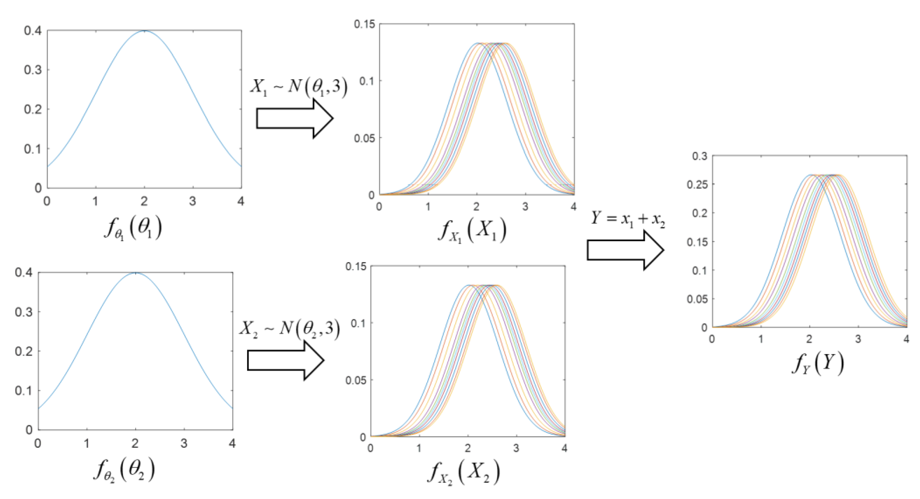
2. Problem Formulation

The computational model of an engineering system is available, the performance function $Y=g\left(X\right)$ can be calculated using theoretical analysis, finite element analysis, or experimental calculation. $X=\left(X_1,\cdots ,X_n\right)$ is the vector of n independent uncertain input variables.

In the probabilistic framework, the uncertainty of input variables $X$ can be represented with the probability density function (PDF) $f_X\left(X\right)$. The corresponding performance function Y is also uncertain, whose PDF $f_Y\left(Y\right)$ can be calculated through uncertainty propagation analysis. For the uncertain input variables $X$ with determinate distribution types and distribution parameters $\mathsf{\theta }$, the PDF $f_X\left(X\right)$ is also determinate. However, in some situations, the uncertainty representation data and uncertainty information are insufficient, and the uncertainty variables are represented by sparse variables with uncertain distribution types or distribution parameters [41,42]. For the sake of simplification, the distribution types are assumed to be determinate. Only uncertainties of distribution parameters $\mathsf{\theta }$ are analyzed, which can be represented by PDF $f_{\mathsf{\theta }}\left(\mathsf{\theta }\right)$, where $\mathsf{\theta }=\left({\theta }_1,\cdots ,{\theta }_p\right)$ is the vector of p independent distribution parameters. For instance, the distribution type of $X_l$ is a normal distribution, and there are two distribution parameters, which are the mean ${\theta }_1$ and standard deviation ${\theta }_2$.

As shown in Figure 1, when considering the uncertainty of distribution parameters $\mathsf{\theta }$, the PDF of input variables $X$ is a family of PDFs, which is the uncertainty function of distribution parameters $\mathsf{\theta }$, which can be expressed as $f_X\left(X|\mathsf{\theta }\right)$. The corresponding PDF of performance function $Y$ is also a family of PDFs. For every value of $\mathsf{\theta }$, the PDF of $X$ and corresponding PDF of $Y$ can be calculated, using uncertainty propagation methods. The uncertain distribution parameters $\mathsf{\theta }$ and input variables $X$ are continuous real numbers, and the performance function $Y$ is also a continuous variation function. Therefore, the performance function $Y=\psi \left(\mathsf{\theta }\right)$ between distribution parameters $\mathsf{\theta }$ and performance function $Y$ is also a continuous square integrable function of distribution parameters $\mathsf{\theta }$. The uncertainty representation function of $Y$ under every value of $\mathsf{\theta }$ can be calculated, using uncertainty propagation methods. However, the function $\psi$ is complex and cannot be obtained by an analytical model, but it can be represented by an approximate model or numerical method. There are some new challenges when considering the uncertainty of distribution parameters $\mathsf{\theta }$:

(1)

There is a nested double loop in the uncertainty analysis of performance function $Y$, which is complex and computationally expensive. With the increase in the total number $p$ of $\mathsf{\theta }$, the computational time increases exponentially. For example, there are 10 uncertainty variables, which have 2 uncertainty distribution parameters for every uncertainty variables. The sampling points for every distribution parameter is 1000. For considering the uncorrelation between 20 distribution parameters, the total sampling point of uncertainty distribution parameters is increased along with the number of distribution parameters; therefore, the total sampling point of distribution parameters is 20 × 1000 = 2 × 10⁴; For every group of sampling points of distribution parameters, the sampling points of 10 uncertainty variables is 10 × 1000 = 10⁴. The total number of sampling points will, therefore, be $2\times {10}^8$, which is time-consuming, especially for an engineering system whose performance function at every sampling point is difficult to calculate or analyze.

(2)

Considering the uncertainty of distribution parameters $\mathsf{\theta }$, the performance function $Y$ is a function of uncertain input variables $X$ and distribution parameters $\mathsf{\theta }$ simultaneously. Therefore, the SA of $X$ and $\mathsf{\theta }$ should be analyzed. The analytical expression of function $\psi$ is difficult to obtain. Therefore, calculating the SA values is another challenge.

According to the classical variance based sensitivity analysis method, the sensitivity between uncertain input variables $X$ and output performance function $Y$ can be represented using two indices: the first-order sensitivity index $S_{X_l}$ and total sensitivity index $S_{T{X}_l}$.

The first-order sensitivity index $S_{X_l}$ measures the variation of the output performance function $Y$ associated with variations in input variable $X_l$ and without other input variables [44,45].

$$S_{X_l}=\frac{V_{X_l}\left[E_{X_{-l}}\left(Y|X_l\right)\right]}{V\left(Y\right)},$$

(1)

where $V_{X_l}\left[E_{X_{-l}}\left(Y|X_l\right)\right]$ measures the average residual variance of the model output when $X_l$ is fixed through its full distribution range, and $X_{-l}$ represents a vector including all input variables, except $X_l$.

Similarly, the total sensitivity index $S_{T{X}_l}$ measures the total impact of uncertain input variables $X_l$, which contain the independent and interaction with other variables [46,47].

$$S_{T{X}_l}=1-\frac{V_{X_{-l}}\left[E_{X_l}\left(Y|X_{-l}\right)\right]}{V\left(Y\right)}=\frac{E_{X_{-l}}\left[V_{X_l}\left(Y|X_{-l}\right)\right]}{V\left(Y\right)},$$

(2)

The total sensitivity index $S_{T{X}_l}$ can be calculated based on the first-order sensitivity index of $S_{X_{-l}}$. Therefore, for simplicity, only the first-order sensitivity indices of input variables and distribution parameters are analyzed and calculated.

Considering the influence of uncertain distribution parameters $\mathsf{\theta }$, the output variance and the corresponding variance contribution can be analyzed using the high dimensional representation method. The expected value of output variance is decomposed to eliminate the influences of uncertain distribution parameters $\mathsf{\theta }$. Since the output variance and the variance contributions are averaged in the parameter space, the first-order sensitivity index of input variables $S_{X_l}$ in Equation (1) is transformed into Equation (3); the details are explained by Wang [43]. There is a functional relationship between the output statistical values and uncertain distribution parameters. In Equation (1), $S_{X_l}$ is calculated based on the functional relationship between x and y. Similarly, based on the functional relationship $\psi$ between θ and y, the first-order sensitivity index of distribution parameters $S_{{\theta }_i}$ is defined in Equation (4).

$$S_{X_l}=E_{{\theta }_i}\left\{V_{X_l}\left[E_{X_{-l}}(Y|X_l)\right]\right\},$$

(3)

$$S_{{\theta }_i}=V_{{\theta }_i}\left[E_{{\mathsf{\theta }}_{-i}}(\psi (\mathsf{\theta })|{\theta }_i)\right],$$

(4)

The first-order sensitivity indices $S_{X_l}$ and $S_{{\theta }_i}$ can identify the influence of input variables and distribution parameters on the output variance. However, there are difficulties in the specific calculation of these sensitivity indices: (1) it is impossible to obtain the explicit function of $\psi$, and the calculation of the mean and variance under some constraints in Equation (4) is difficult; and (2) the nested double loop of sampling for uncertain input variables and distribution parameters increases the computational complexity and decreases the computational efficiency. To solve these issues, a sampling-based sensitivity analysis method is presented here. The Gaussian integral formula was improved by incorporating the unscented transformation method [48] to solve the sensitivity analysis problem considering uncertainties of input variables and their distribution parameters simultaneously.

3. An Efficient Sampling-Based SA Method Based on Unscented Transformation

The first-order sensitivity index of input variables $S_{X_l}$ can be equivalently converted to Equation (5), according to the algorithm in [49].

$$S_{X_l}=E_{{\theta }_i}\left\{V_{X_l}\left[E_{X_{-l}}(Y|X_l)\right]\right\}=E_{{\theta }_i}\left\{V(Y)-E_X{\left[g\left(X\right)-E_{X_{-l}}(Y|X_l)\right]}^2\right\},$$

(5)

The three-loop sampling procedure is involved in the calculation of Equation (5). In the first loop, $X_{-l}$ are sampled for determinate $X_l$, and the conditional expectation $E_{X_{-l}}(Y|X_l)$ is calculated. In the second loop, $X$ are sampled for determinate distribution parameters $\mathsf{\theta }$, and the conditional expectation $E_X{\left[g\left(X\right)-E_{X_{-l}}(Y|X_l)\right]}^2$ and total variance $V\left(Y\right)$ are calculated. In the third loop, distribution parameters $\mathsf{\theta }$ are sampled according to their probability density function $f_{\mathsf{\theta }}\left(\mathsf{\theta }\right)$, and the first-order sensitivity index $S_{X_l}$ is obtained.

There are many approximation methods to reduce the sampling number in the sampling loops, such as spline Gaussian rules [50,51,52,53] and polynomial rules [49,54]. The spline Gaussian rules are exact for a sufficiently smooth integrand and spline rules, they require fewer integration points, and have been widely used in isogeometric analysis. However, the accuracy of uncertain sensitivity indices is more important than the accuracy of sampling curves in these problems. Polynomial rules have been proved in many uncertainty analysis problems; therefore, a new sampling method based on multiplication approximation [54] and the unscented transformation method is proposed to convent the inner two loops into one loop. The multiplication approximation method is a conventional dimensional reduction method, which assumes that the influence of higher-order terms is smaller than that of the univariate terms. In the uncertainty analysis, we mainly focused on the first-order sensitivity analysis in which the influences of higher-order terms are lower than those of one-dimensional terms. Therefore, the conditional expectation $E_{X_{-l}}(Y|X_l)$ in the first loop can be approximately expressed in Equation (6), based on the multiplication approximation method.

$$\begin{array}{l}{E}_{X_{-l}}(Y|X_l)={\displaystyle \int g(X)}{f}_{X_{-l}}(X_{-l})d{x}_{-l}\\ \approx {[g(c)]}^{1-n}\cdot g(c_1,\dots ,c_{l-1},x_l,c_{l+1},\dots ,c_n)\times {\displaystyle \prod _{\begin{array}{l}j=1\\ j\ne l\end{array}}^n{\displaystyle {\int }_{X_j}g}}(c_1,\dots ,c_{j-1},x_j,c_{j+1},\dots ,c_n)f_{X_j}(x_j)d{x}_j\\ =g{[(c)]}^{-1}g(c_1,\dots ,c_{l-1},x_l,c_{l+1},\dots ,c_n)\times {\displaystyle \prod _{\begin{array}{l}j=1\\ j\ne l\end{array}}^n{E}_{X_{\mathrm{j}}}}\end{array}$$

(6)

where the reference points $c=\left[c_1,c_2,\cdots ,c_n\right]$, and $c_l$ is the mean value of uncertain input variable $X_l$. $E_{X_j}$ is a one-dimensional integration function. In the traditional method, $E_{X_j}$ is calculated using the Monte-Carlo method or the Gaussian integration method, which need a large number of sampling points. Therefore, a new sampling method based on the unscented transformation method is proposed to calculate $E_{X_j}$ with few sampling points.

The sampling intervals of uncertain input variables $X_l$ are determined by $3\sigma$ criterions. The mean ${\mu }_{X_l}$ and standard deviation ${\sigma }_{X_l}$ of $X_l$ are determined based on the probability density function $f_{X_l}\left(X_l\right)$. The sampling interval $\left[{\mu }_{X_l}-3{\sigma }_{X_l},{\mu }_{X_l}+3{\sigma }_{X_l}\right]$ is equally probabilistically divided into $N^{\prime }$ subintervals that do not overlap each other and that fill the entire value area. Every subinterval is divided into (2n + 1) cells, where the adaptive sigma points and corresponding weight ratios are determined using the unscented transformation method. The calculation algorithm of $E_{X_j}$ can be approximated in Equation (7).

$$E_{X_j}={\displaystyle {\int }_{X_j}g}(c_1,\dots ,c_{j-1},x_j,c_{j+1},\dots ,c_n)f_{X_j}(x_j)d{x}_j\approx {\displaystyle \sum _{k=1}^{N\prime }{\displaystyle \sum _{m=1}^{2n+1}g(c_1,\dots ,c_{j-1},s_j{}^{m,k},c_{j+1},\dots ,c_n)f_{X_j}(s_{{}_j}^{m,k})\cdot d_{{}_{s_j}}^m}},$$

(7)

where $d$ is the step size of the k- subinterval of the Gaussian distribution sampling interval $\left[{\mu }_{X_l}-3{\sigma }_{X_l},{\mu }_{X_l}+3{\sigma }_{X_l}\right]$, $s_j^{m,k}$ is the sigma points of $X_j$, and $d_{{}_{s_j}}^m=d_{}/\left(2n+1\right)$ is the cell step size in the k-th subinterval.

The sigma points $s_j^{m,k}$ and corresponding weights $W_j^{m,k}$ in k-th sub-intervals are determined using the algorithm as follows: the mean ${\overline{X}}_j$ and variance-covariance matrix $P_{XX}$ of uncertain input variables in the k-th sub-intervals are calculated based on $f_X\left(X\right)$. The 2n + 1 sampling points $s_j^{m,k}\left(m=1,\cdots ,2n+1\right)$ in the k-th sub-intervals are determined using Equations (8) and (9) based on the standard unscented transformation algorithm [55].

$$s_j^{0,k}=W_0{\overline{X}}_j,$$

(8)

$$s_j^{m,k}=\{\begin{array}{ll}{\overline{X}}_j+{\left(\sqrt{\frac{n}{1-W_0}{P}_{XX}}\right)}_m\hfill & m\in \left[1,n\right]\hfill \\ {\overline{X}}_j-{\left(\sqrt{\frac{n}{1-W_0}{P}_{XX}}\right)}_m\hfill & m\in \left[n+1,2n+1\right]\hfill \end{array},$$

(9)

where $W_0$ is the initial weight ratio, $\sqrt{}$ is a matrix square root, and ${\left(\right)}_m$ is the m-th row of the matrix. The variance–covariance matrix $P_{XX}$ is calculated using Equation (10).

$$P_{XX}={\displaystyle \sum _{j=1}^n{W}_j^{m,k}\left(s_j^{m,k}-\overline{X}\right){\left(s_j^{m,k}-\overline{X}\right)}^T},$$

(10)

The weight ratios $W_j^{m,k}$ of sampling points $s_j^{m,k}$ are determined using Equation (11).

$$W_{{}_j}^{m,k}=\{\begin{array}{ll}{W}_0\hfill & m=0\hfill \\ \left(1-W_0\right)/2n\hfill & m=1,\cdots ,2n+1\hfill \end{array},$$

(11)

After determining the sampling points $s_j$ and corresponding weight ratios $W_j$ in m-th cell, $E_{X_j}$ can be calculated using single-loop sampling points. The total number of sampling points is $\left(2n+1\right)N\prime$, where $n$ is the number of uncertain input variables, and $N\prime$ is the subintervals number of $\left[{\mu }_{X_l}-3{\sigma }_{X_l},{\mu }_{X_l}+3{\sigma }_{X_l}\right]$.

The sensitivity index of distribution parameters $S_{{\theta }_i}$ can be transformed from Equation (4) to Equation (12), using a similar convention method as used for uncertain input variables $X$.

$$S_{{\theta }_i}=V\left(\psi \right)-E_{{\theta }_i}{\left[g\left(X\right)-E_{{\mathsf{\theta }}_{-i}}(\psi |{\theta }_i)\right]}^2,$$

(12)

In the calculation of Equation (12), four input factors need to be sampled, which contain the sampling of ${\theta }_i$, ${\mathsf{\theta }}_{-i}$, input variable of ${\theta }_i$ and other input variables. After determining the sampling points, a large number of Monte Carlo sampling points is used to calculate conditional expectation $E_{{\theta }_i}{\left[g\left(X\right)-E_{{\mathsf{\theta }}_{-i}}(\psi |{\theta }_i)\right]}^2$. To decrease the computational complexity, a similar calculation method to that for $S_{X_l}$ is implemented to calculate $S_{{\theta }_i}$, and the details are presented in Section 4.2.

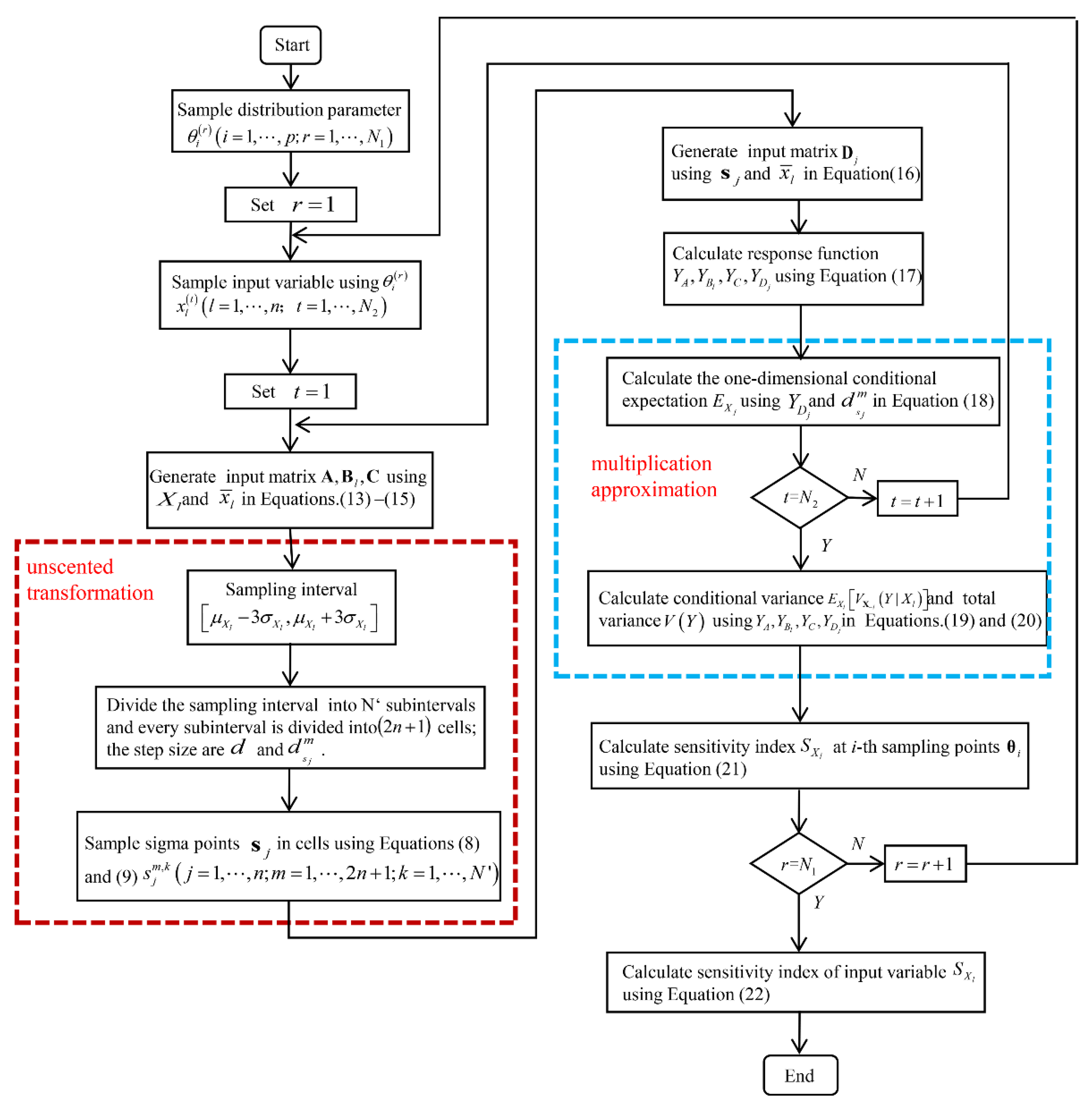
4. Implementation of the Proposed Sensitivity Calculation Algorithm

4.1. Calculation of the First-Order Sensitivity Index of the Input Variables

The detailed procedures for calculating the first-order sensitivity index of input variables $S_{X_l}$ are given below, and the flowchart is given in Figure 2.

Step 1: In the outer loop, $N_1$ sampling points ${\theta }_i^{\left(r\right)}\left(i=1,\cdots ,p;r=1,\cdots ,N_1\right)$ for uncertain distribution parameters θ are determined according to their probability density functions $f_{\mathsf{\theta }}\left(\mathsf{\theta }\right)$.

Step 2: At every sampling point ${\theta }_i^{\left(r\right)}$, the uncertainty information and probability density function of input variables $X$ are determined. $N_2$ sampling points of $x_l^{\left(t\right)}\left(l=1,\cdots ,n;t=1,\cdots ,N_2\right)$ are generated according to the joint probability density function $f_X\left(X\right)$ with determining distribution parameters $\mathsf{\theta }$. The $N_2\times n$ sampling matrix $A$ of uncertain input variables $X$ are generated in Equation (13).

$$A=\left[\begin{array}{cccc}{x}_1^{(1)}& x_1^{(2)}& \cdots & x_1^{\left(N_2\right)}\\ x_2^{(1)}& x_2^{(2)}& \cdots & x_2^{\left(N_2\right)}\\ ⋮& ⋮& \ddots & ⋮\\ x_n^{(1)}& x_n^{(2)}& \cdots & x_n^{\left(N_2\right)}\end{array}\right],$$

(13)

Step 3: The reference point $c$ is generated in Equation (14), and the sampling value of every uncertain input variable $X_l$ is its mean value ${\overline{x}}_l$.

$$c={\left[{\overline{x}}_1,{\overline{x}}_2,\cdots ,{\overline{x}}_n\right]}^T,$$

(14)

Step 4: The new sampling matrix $B_l$ is obtained in Equation (15) through assigning reference point $c$ into the column of the matrix $A$ expect the l-th column.

$$B_l=\left[\begin{array}{ccccc}{\overline{x}}_1& \cdots & x_l^{(1)}& \cdots & {\overline{x}}_n\\ {\overline{x}}_1& \cdots & x_l^{(2)}& \cdots & {\overline{x}}_n\\ ⋮& ⋮& ⋮& \ddots & ⋮\\ {\overline{x}}_1& \cdots & x_l^{(N_2)}& \cdots & {\overline{x}}_n\end{array}\right],$$

(15)

Step 5: The sampling interval $\left[{\mu }_{X_l}-3{\sigma }_{X_l},{\mu }_{X_l}+3{\sigma }_{X_l}\right]$ is divided into $N^{\prime }$ subintervals. The sigma points $s_{{}_j}^{m,k}\left(j=1,\cdots ,n;m=1,\cdots ,2n+1;k=1,\cdots ,N^{\prime }\right)$ and corresponding weight ratios $W_{{}_j}^{m,k}$ at every subinterval are obtained based on the algorithm in Equations (8)–(11). The joint probability density function $f_{X_j}\left(s_j\right)$ is estimated according to the selected sigma points $s_j$.

Step 6: New $\left(2n+1\right)\times n$ sampling matrix $D_j$ is obtained in Equation (16). The j-th column is sigma points $s_j^{}$, and other columns are references point $c$.

$$D_j=\left[\begin{array}{ccccc}{\overline{x}}_1& \cdots & s_j^{(1)}& \cdots & {\overline{x}}_n\\ {\overline{x}}_1& \cdots & s_j^{(2)}& \cdots & {\overline{x}}_n\\ ⋮& ⋮& ⋮& \ddots & ⋮\\ {\overline{x}}_1& \cdots & s_j^{(2n+1)}& \cdots & {\overline{x}}_n\end{array}\right],$$

(16)

Step 7: The values of the performance function at the sampling matrices are calculated in Equation (17).

$$Y_A=g\left(A\right),Y_{B_l}=g\left(B_l\right),Y_C=g\left(C\right),Y_{D_j}=g\left(D_j\right),$$

(17)

Step 8: The one-dimensional conditional expectation $E_{X_j}$ in Equation (7) is calculated based on sampling values $D_j$ for selected sigma points $s_j$ in Equation (18).

$$E_{X_j}\approx {\displaystyle \sum _{k=1}^{N\prime }{\displaystyle \sum _{m=1}^{2n+1}g(D_j)\cdot f_{X_j}(s_{{}_j}^{m,k})\cdot d_{{}_{s_j}}^m}},$$

(18)

Step 9: Based on the algorithms in Equations (6) and (7), $E_X{\left[g\left(X\right)-E_{X_{-l}}(Y|X_l)\right]}^2$ and $V\left(Y\right)$ can be calculated, using Equations (19) and (20), respectively.

$$E_{X_l}\left[V_{X_{-l}}\left(Y|X_l\right)\right]=\frac{1}{N_2}{\displaystyle \sum _{t=1}^{N_2}{\left[g{\left(A\right)}_{}^{\left(t\right)}-g{[(c)]}^{-1}g\left(B_l\right)\times {\displaystyle \prod _{\begin{array}{l}j=1\\ j\ne l\end{array}}^n{E}_{s_j}}(G|s_j)\right]}^2},$$

(19)

$$V\left(Y\right)=\frac{1}{N_2}{\displaystyle \sum _{t=1}^{N_2}{\left[g{\left(A\right)}_{}^{\left(t\right)}\right]}^2}-{\left[\frac{1}{N_2}{\displaystyle \sum _{t=1}^{N_2}g{\left(A\right)}_{}^{\left(t\right)}}\right]}^2,$$

(20)

Step 10: At the inner loop, the sensitivity index $S_{X_l}$ at i-th sampling points ${\theta }_i$ of distribution parameters $\mathsf{\theta }$ is approximated by Equation (21) based on Equations (7), (19) and (20).

$$S_{X_l}=\frac{1}{N_2}{\displaystyle \sum _{t=1}^{N_2}{\left[g{(A)}^{\left(t\right)}\right]}^2-}{\left[\frac{1}{N_2}{\displaystyle \sum _{t=1}^{N_2}g{(A)}^{\left(t\right)}}\right]}^2-\frac{1}{N_2}{\displaystyle \sum _{t=1}^{N_2}{\left[g{(A)}^{\left(t\right)}-g{(c)}^{1-n}\cdot g{(B_l)}^{\left(t\right)}\cdot {\displaystyle \prod _{\begin{array}{l}j=1\\ j\ne l\end{array}}^n{E}_{s_j}(G|s_j)}\right]}^2},$$

(21)

Step 11: At the outer loop, the sensitivity index $S_{X_l}$, considering uncertain distribution parameters, is calculated in Equation (22).

$$S_{X_l}=\frac{1}{N_1}{\displaystyle \sum _{r=1}^{N_1}\left\{\frac{1}{N_2}{\displaystyle \sum _{t=1}^{N_2}{\left[g{(A)}^{\left(t\right)}\right]}^2-}\left[\frac{1}{N_2}{\displaystyle \sum _{t=1}^{N_2}g{(A)}^{\left(t\right)}}\right]-\frac{1}{N_2}{\displaystyle \sum _{t=1}^{N_2}{\left[g{(A)}^{\left(t\right)}-g{(c)}^{1-n}\cdot g{(B_l)}^{\left(t\right)}\cdot {\displaystyle \prod _{\begin{array}{l}j=1\\ j\ne l\end{array}}^n{E}_{s_j}(G|s_j)}\right]}^2}\right\}},$$

(22)

Step 12: To decrease the random errors due to the selection of random sampling points, Steps 1–11 are implemented repeatedly, and the means of the sensitivity indices are the final, first-order sensitivity index of the input variables.

4.2. Calculation of the First-Order Sensitivity Index of the Distribution Parameters

To effectively calculate the first-order sensitivity index of distribution parameters $S_{{\theta }_i}$, the three-loop sampling method was implemented, and the flowchart is shown in Figure 3. The steps are as follows.

Step 1: In the first loop, $N_1$ sampling points ${\theta }_i^{\left(r\right)}\left(i=1,\cdots ,p;r=1,\cdots ,N_1\right)$ for uncertain distribution parameter ${\theta }_i$ are determined based on its probability density function.

Step 2: In the second loop, the corresponding input variable of distribution parameter ${\theta }_i$ is assumed as to be $X_l$. $N_2$ sampling points $x_l^{\left(t\right)}\left(l=1,\cdots ,n;t=1,\cdots ,N_2\right)$ for uncertain input variable $X_l$ are obtained with the determinate distribution parameter sampling value ${\theta }_i^{\left(r\right)}$. Other uncertain distribution parameters ${\mathsf{\theta }}_{-i}$ are sampled according to their probability density function, and $N_1$ sampling points ${\theta }_{-i}^{\left(rr\right)}\left(i=1,\cdots ,p;rr=1,\cdots ,N_1\right)$ are obtained.

Step 3: In the third loop, $N_2$ sampling points of other uncertain input variables $X_{-l}$ are obtained according to their probability density function with determinate distribution parameters ${\mathsf{\theta }}_{-i}^{}$. Therefore, the sampling matrices $A$, $B_l$, and $D_j$ are selected and the corresponding output values $Y_A,Y_{B_l},Y_C,Y_{D_j}$ are calculated, using Equations (13)–(17) in Section 4.1.

Step 4: The total variance $V\left(\psi \right)$ is calculated using all sampling values of $Y_A$ in three sampling loops of all uncertain input variables and uncertain parameters, which is shown in Equation (23).

$$V\left(\psi \right)=\frac{1}{{\left(N_1\right)}^p\times N_2}{\displaystyle \sum _{}^{}{\left(Y_A\right)}^2}-{\left[\frac{1}{{\left(N_1\right)}^p\times N_2}{\displaystyle \sum _{}^{}\left(Y_A\right)}\right]}^2,$$

(23)

where $p$ is the number of uncertain distribution parameters, $N_1$ is the number of samples of each uncertainty distribution parameter ${\theta }_i$, and $N_2$ is the number of samples of each uncertainty input variable $X_l$. Therefore, the total number of samples ${\left(N_1\right)}^p{N}_2$ for calculating the total variance of the determinate input variable $X_l$ is the multiplication of the number of samples of all the uncertain distribution parameters and the number of samples of the input variable.

Step 5: In the calculation of $E_{{\theta }_i}{\left[g\left(X\right)-E_{{\mathsf{\theta }}_{-i}}(\psi |{\theta }_i)\right]}^2$, the unscented transformation method is also used. In the third loop, the sampling interval $\left[{\mu }_{X_l}-3{\sigma }_{X_l},{\mu }_{X_l}+3{\sigma }_{X_l}\right]$ of uncertain input variables $X_l$ is equally probabilistically divided into $N^{\prime }$ subintervals. Every subinterval is divided into $\left(2n+1\right)$ cells, where the adaptive sigma points $s_j^{m,k}\left(j=1,\cdots ,n;m=1,\cdots ,2n+1;k=1,\cdots ,N\prime \right)$ and the corresponding weight ratios are determined using the unscented transformation method. The output performance function is calculated using $g\left(D_j\right)$. Then, the conditional expectation $E_{s_j}(G|s_j)$ and $E_{{\mathsf{\theta }}_{-i}}(\psi |{\theta }_i)$ are calculated, using Equations (24) and (25), respectively. Therefore, the expectation $E_{{\theta }_i}{\left[g\left(X\right)-E_{{\mathsf{\theta }}_{-i}}(\psi |{\theta }_i)\right]}^2$ can be calculated in Equation (26).

$$\begin{array}{c}{E}_{s_j}(G|s_j)={\displaystyle {\int }_{}g(c_1,\dots ,c_{j-1},s_j,c_{j+1},\dots ,c_n)f_{X_j}(s_j)d{s}_j}\\ ={\displaystyle \sum _{k=1}^{N\prime }{\displaystyle \sum _{m=1}^{2n+1}g(D_j)\cdot f_{X_j}(s_j^{m.k})\cdot d_{{}_{s_j}}^m}}\end{array}$$

(24)

$$E_{{\mathsf{\theta }}_{-i}}(\psi |{\theta }_i)={[g(c)]}^{1-n}g\left(B_l\right)\times {\displaystyle \prod _{\begin{array}{l}j=1\\ j\ne i\end{array}}^n{E}_{s_j}}(G|s_j),$$

(25)

$$E_{{\theta }_i}\left[V_{{\mathsf{\theta }}_{-i}}\left(\psi |{\theta }_i\right)\right]=\frac{1}{{\left(N_1\right)}^p\times N_2}{\displaystyle \sum _{}^{}{\left[g(A)-g{[(c)]}^{1-n}g\left(B_l\right)\times {\displaystyle \prod _{\begin{array}{l}j=1\\ j\ne l\end{array}}^n{E}_{s_j}(G|s_j)}\right]}^2},$$

(26)

Step 6: The results in the third loop are integrated into the first sampling loop of distribution parameter ${\theta }_i$ and the second sampling loop for ${\mathsf{\theta }}_{-i}$. The first-order sensitivity index of distribution parameter $S_{{\theta }_i}$ is calculated in Equation (27).

$$S_{{\theta }_i}=\frac{1}{{\left(N_1\right)}^p\times N_2}{\displaystyle \sum _{}^{}{\left[g(A)\right]}^2-}{\left[\frac{1}{{\left(N_1\right)}^p\times N_2}{\displaystyle \sum _{}^{}g{(A)}^{}}\right]}^2-\frac{1}{{\left(N_1\right)}^p\times N_2}{\displaystyle \sum _{}^{}{\left[g{(A)}^{}-g{(c)}^{1-n}\cdot g({{\rm B}}_l)\cdot {\displaystyle \prod _{\begin{array}{l}j=1\\ j\ne l\end{array}}^n{E}_{s_j}(G|s_j)}\right]}^2}$$

(27)

4.3. Computational Effort and Comparison to the Crude Monte-Carlo

The computational cost of the sampling-based sensitivity analysis methods mainly depends on the estimation of the performance function $Y$ at the sampling points.

In the computation of sensitivity indices of input variables $S_{X_l}$, the sampling numbers of uncertain distribution parameters $\mathsf{\theta }$ and input variables $X$ are $N_1$ and $N_2$, respectively, and the corresponding $Y_A$ and $Y_{B_l}$, are estimated. At every sampling point of the distribution parameters ${\theta }_i$, $\left(2n+1\right)$ sigma sampling points for $N^{\prime }$ subintervals and reference point $c$ are selected, and the corresponding $Y_{Dj}$ and $Y_C$ are calculated to determine the one-dimensional conditional expectation $E_{s_j}(G|s_j)$. Therefore, the total number of model evaluations $N_{X-p}$ for $S_{X_l}$ in the proposed method is given in Equation (28).

$$N_{X-p}=N_1\left[N_2\left(n+1\right)+(2n+1)N\prime +1\right],$$

(28)

Using traditional single-loop Monte Carlo sampling (MCS) [56] to calculate $S_{X_l}$, the total number of model evaluations is $N_1\left[N_2\left(n+2\right)\right]$. The subinterval number $N^{\prime }$ is about 10–30, which is far less than the sampling number $N_2$ (100~1000) of uncertain input variables $X_l$. Therefore, the total evaluation number is decreased, and the computational efficiency is improved through using the proposed algorithm.

In the computation of the sensitivity indices of distribution parameters $S_{{\theta }_i}$, the model evaluation number for $E_{s_j}(G|s_j)$ is the same as that in the calculation of $S_{X_l}$, which is $(2n+1)N\prime +1$. The sampling number of distribution parameters ${\theta }_i$ is ${\left(N_1\right)}^p$, and the evaluation number of $Y_A$ and $Y_{B_l}$ are $N_{{}_2}^{}$ and $n{N}_{{}_2}^{}$, respectively. Therefore, the total number of model evaluations $N_{\theta -p}$ is given in Equation (29).

$$N_{\theta -}{}_p=N_{{}_2}^{}{\left(N_{{}_1}^{}\right)}^p\left[N_{{}_2}^{}\left(n+1\right)+(2n+1)N\prime +1\right],$$

(29)

In the MCS method, the total number of model evaluations is $\left(n+2\right)N_{{}_2}^{}{\left(N_{{}_1}^{}\right)}^p$, where $N_1$ and $N_2$ are the sampling number of distribution parameter ${\theta }_i$ and input variable $X_l$, respectively. The values of $N_1$ and $N_2$ are about ${10}^4$ in the MCS method. In the proposed method, the model can converge, and accurate sensitivity indices can be acquired when the number of both $N_1$ and $N_2$ are about 100. Therefore, the total number of model evaluations is decreased, and the computational efficiency is improved, in terms of the accuracy of the results for the sensitivity indices of the uncertain distribution parameters, through using the proposed algorithm.

5. Numerical and Engineering Examples

Four examples are used to illustrate the effectiveness of the proposed methodology. In numerical example 1, the uncertain input variables are independent, and the cross terms among the uncertain input variables are considered in numerical example 2. Arbitrary distribution types of uncertain input variables and distribution parameters can be analyzed by the proposed methodology; therefore, the normal distribution and Gamma distribution types are handled in numerical example 3. The example of a heat exchanger can illustrate this method’s effectiveness in complex, actual engineering conditions.

5.1. Numerical Example 1

Let us consider the quadratic polynomial model without cross terms in Equation (30).

$$Y=40-18X_1+X_2^2+X_2+X_3^2+5X_3,$$

(30)

where $X_l\sim N\left(\theta ,1\right),l=1,2,3$ are independent uncertain input variables with normal distribution type, and their standard deviations are determinate values. The mean values of $X_l$ are the same as $\theta \sim N\left(4,1\right)$, which is a normal distribution function with a mean of 4 and a standard deviation of 1.

The first-order sensitivity indices of uncertain input variables and distribution parameters were estimated using the proposed methodology and MCS method. The mean absolute errors (MAE) of $X$ are shown in Figure 4 under different numbers of total sampling points for the proposed algorithm and the MCS method. The MAE for the MCS method is unstable because there are many randomicities in the sampling procedure. However, the MAE of the proposed methodology decreased as the total number of sampling points increased, which was less than that of MCS when the total number of sampling points was higher than 7 × 10⁴. The calculated first-order sensitivity indices are listed in

Table 1. First-order sensitivity indices in Example 1.

Sensitivity Indices	Accurate Values	Proposed Method	${\mathit{\epsilon }}_{\mathit{p}\mathit{r}\mathit{o}}$	MCS	${\mathit{\epsilon }}_{\mathit{M}\mathit{C}\mathit{S}}$
$S_{X_1}$	324	324.30	0.09%	323.91	0.03%
$S_{X_2}$	87	86.96	0.05%	87.13	0.15%
$S_{X_3}$	175	175.05	0.03%	176.06	0.60%
$S_{{\theta }_1}$	0	0	0	0	0
$S_{{\theta }_2}$	1328	1316.32	0.89%	1323.52	0.34%
$S_{{\theta }_3}$	2736	2879.15	4.97%	2864.03	4.47%

. The accurate values of the first-order sensitivity indices were also calculated using the analytic method in [43], which are also listed in Table 1. The proposed method and MCS method can both obtain accurate sequences of the sensitivity indices, which were $S_{X_1}>S_{X_3}>S_{X_2}$ for uncertain input variables and $S_{{\theta }_3}>S_{{\theta }_2}>S_{{\theta }_1}$ for uncertain distribution parameters. The maximum relative errors for $S_X$ were 0.09% and 0.60% for the proposed method and MCS method, respectively, while the maximum relative errors for $S_{\theta }$ were 4.97% and 4.47%, respectively. The proposed method can also obtain accurate sensitivity indices when the sampling points decrease from $5\times {10}^8$ to 61,000, which can decrease the computational number of the performance function and improve the computational efficiency. Through using the proposed method, the first-order sensitivity indices can be estimated accurately with fewer sampling points than that required for the MCS method.

5.2. Numerical Example 2

A polynomial model with cross terms in Equation (31) was analyzed.

$$Y=X_1+2X_2+3X_1{X}_2,$$

(31)

where $X_1\sim N\left({\theta }_1,2\right)$ and $X_2\sim N\left({\theta }_2,1\right)$ are uncertain input variables with normal distribution type. The mean values ${\theta }_1\sim N\left(1,1\right)$ of $X_1$ and ${\theta }_1\sim N\left(2,1\right)$ of $X_2$ are normal distribution types with determinate distribution parameters.

The proposed method and traditional MCS method were used to calculate the first-order sensitivity indices. The MAEs under the same number of total sampling points for the proposed method and MCS method are shown in Figure 5. As the number of sampling points increased, the accuracy of the calculated results improved. The proposed method can obtain more accurate results compared with the MCS method with the same number of total sampling points. The proposed method can obtain accurate first-order sensitivity indices with $3\times {10}^4$ sampling points, while the MCS method required $4\times {10}^8$ sampling points. The proposed method needed fewer sampling points, which improved the computational efficiency. The calculated first-order sensitivity indices for uncertain input variables and distribution parameters are shown in Figure 6. The accurate analytical results and SDP results in [43] are also shown in Figure 6. The maximum relative errors of $S_X$ and $S_{\theta }$ for the proposed method were 2.94% and 2.31%, respectively, which are not only lower than 5.88% and 12.99% for the MCS method, but are also lower than 12. 82% and 4.91% for the SDP method.

5.3. Numerical Example 3

A mathematical function with multiple different types of uncertain information was considered, as shown in Equation (32).

$$Y=4-X_1-X_2,$$

(32)

where the uncertain input variable $X_1\sim N\left({\theta }_1,1\right)$ is a normal distribution variable with an uncertain mean ${\theta }_1$ and determinate standard deviation and $X_2\sim N\left({\theta }_2,1\right)$ is a normal distribution variable with an uncertain mean ${\theta }_2$ and determinate standard deviation. The uncertain distribution parameter ${\theta }_1\sim G\left(3,1\right)$ is a Gamma distribution function, and ${\theta }_2\sim G\left(6,1\right)$ is also a Gamma distribution function.

As there are normal and Gamma distributions in the uncertain input variables and distribution parameters, it is difficult to calculate the first-order sensitivity indices using the analytical method. Therefore, only the proposed method and MCS method were used to calculate the sensitivity indices. In the proposed method, the sampling points for $X_1$, $X_2$, ${\theta }_1$, and ${\theta }_2$ were set as 30, 30, 60, 60, respectively. The total number of sampling points required to calculate the sensitivity of the uncertainty input variables was 18,000, and the total number of sampling points required to calculate the sensitivity of the uncertainty distribution parameters was $2.6\times {10}^7$. In the MCS method, to obtain accurate results, $4\times {10}^8$ sample points were used to calculate the sensitivity of the uncertainty input variables, and $4\times {10}^{12}$ sample points were used to calculate the sensitivity of the uncertainty distribution parameters. The total number of sampling points and calculation number of performance function Y were decreased through using the proposed method. The calculated sensitivity indices are listed in

Table 2. First-order sensitivity indices in Example 3.

Sensitivity Indices	Proposed Method	MCS	$\mathit{\epsilon }$
$S_{X_1}$	0.47	0. 48	2.13%
$S_{X_2}$	0.11	0. 12	9.10%
$S_{{\theta }_1}$	0.92	0. 93	1.09%
$S_{{\theta }_2}$	0.73	0. 70	4.11%

. The maximum relative error of the proposed method was 9.10%, which illustrates the effectiveness of the proposed method. Compared with the theoretical analytical method, the proposed method can manage multiple different distribution types of uncertain input variables and distribution parameters. Compared with the MCS method, the proposed method can generate accurate sensitivity indices with fewer sampling points, which can increase the computational efficiency.

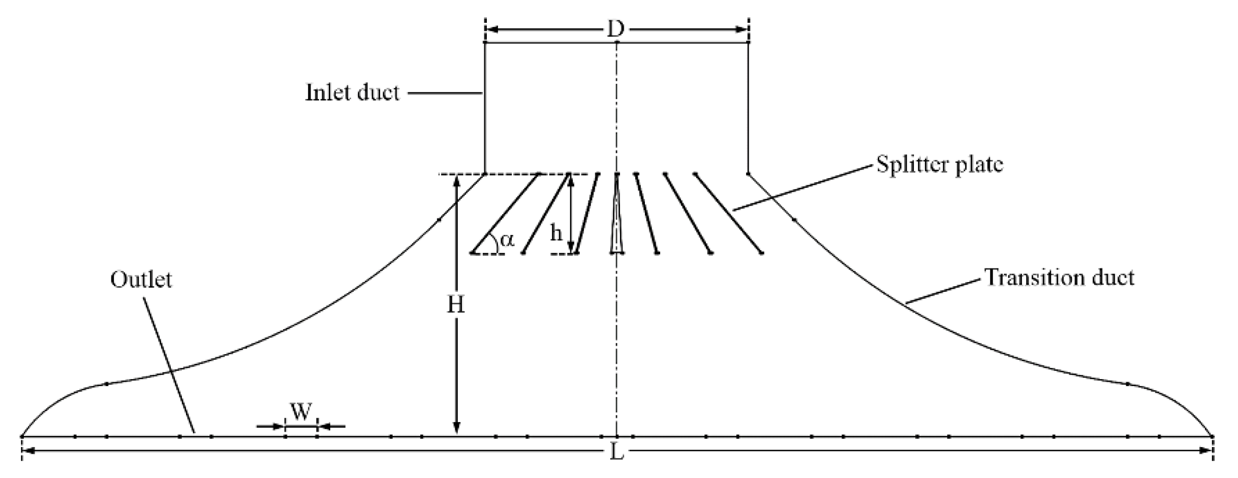
5.4. Engineering Example: Inlet Header of Heat Exchanger

The aforementioned numerical examples are intended to illustrate the effectiveness of the proposed method. In this example, the inlet header of the heat exchanger is employed as an example to illustrate the applicability of the proposed sensitivity analysis method in an engineering application.

The inlet header in Figure 7 is the main component of the heat exchanger. The hot and cold streams flow from the inlet header to the fin channels, and then heat is transferred into the fin channels. Flow maldistribution in the inlet header is one of main factors affecting the total heat transfer rates. The details of the inlet header and heat exchangers can be found in [57,58]. Many structure parameters can influence the flow distribution in the inlet header, and two structure parameters are analyzed in this example: the splitter plate height $h$ and inclined angle of outermost splitter plate $\alpha$. The flow distribution in the inlet header under different $h$ and $\alpha$ values was analyzed in Fluent (Figure 8), and the flow maldistribution degree $S$ was calculated based on the mass flow rate at the outlet region of the inlet header.

Firstly, 25 sampling points of $h$ and $\alpha$ are selected using the Latin hypercube sampling method in the design region $h\in \left[20,40\right]\mathrm{mm}$ and $\alpha \in \left[{46}^{\circ },{54}^{\circ }\right]$. Then, the structure model at these sampling points are constructed in Solidworks, and the flow analysis is implemented in Fluent; the corresponding flow maldistribution degrees S are calculated based on the Fluent analysis results. A total of 20 sampling results are used to fit the response surface model of S, and an additional 5 sampling results are used to verify the accuracy of approximate model. The final approximate response surface model of flow maldistribution degree S is represented by Equation (33).

$$S=61590-382h-2131\alpha +5h^2+21{\alpha }^2,$$

(33)

There were some manufacturing and assembly errors in the inlet header; $h$ and $\alpha$ are uncertain variables. The splitter plate height $h$ was assumed to be $h~N\left({\theta }_1,3\right)\mathsf{m}\mathsf{m}$, and the distribution parameter ${\theta }_1~N\left(30,1\right)\mathsf{m}\mathsf{m}$ was also an uncertain variable with a normal distribution type. The inclined angle $\alpha$ was assumed to be $\alpha ~N\left({\theta }_2,1\right)$, and the distribution parameter ${\theta }_2~N\left({50}^{\circ },1^{\circ }\right)$ was also an uncertain variable with a normal distribution type.

The proposed method and MCS method were used to calculate the sensitivity indices, and the results are listed in

Table 3. First-order sensitivity indices for the inlet header of the heat exchanger.

Sensitivity Indices	Proposed Method	MCS
$S_h$	0.95	0.95
$S_{\alpha }$	0.05	0.05
$S_{{\theta }_1}$	0.95	0.93
$S_{{\theta }_2}$	0.78	0.76

. The maximum relative error of the sensitivity indices between the proposed method and MCS method was 3.22%, which indicated the effectiveness of the proposed method. The total sampling number in the calculation of the sensitivity indices were 21,600 for the proposed method and $4\times {10}^8$ for the MCS method, which reflects the improvement of the computational efficiency. Therefore, the proposed method can obtain accurate sensitivity analysis results with lower computational times, which is useful for the sensitivity analysis of complex engineering products.

6. Conclusions and Discussion

A sampling-based sensitivity analysis method is proposed, which considers the uncertainties of input variables and their distribution parameters. Through computing the conditional expectation in subintervals with the unscented transformation method, the number of total sampling points and loop numbers were decreased, with the high accuracy maintained. The calculation procedures of the first-order sensitivity indices of the uncertainty input variables and distribution parameters were implemented. Through using the proposed algorithm, sensitivity indices with arbitrary distribution types of uncertain input variables and distribution parameters could be calculated, no matter how complex the engineering model was in terms of uncertain input variables and output performance function. The computational efficiency of the sensitivity analysis was improved with high computational accuracy, compared with the MCS method.

However, there are some limitations to the proposed framework, which could be further studied: (1) the distribution type of uncertain input variables was assumed to be determinate; therefore, more distribution types and mixed distribution types for different input variables could be considered in the sensitivity analysis framework; (2) the total sampling number was decreased through adaptive sampling based on the unscented transformation algorithm—however, as there are many potential sampling rules, determining the most suitable sampling rule and the application of spline Gaussian rules could be researched in the future; and (3) the proposed sensitivity analysis method could be extended to consider multiple types of uncertainty variables, such as aleatory uncertainties, p-box, evidence theory variables, and so forth.

References

1. Yeratapally, S.R.; Glavicic, M.G.; Argyrakis, C.; Sangid, M.D. Bayesian uncertainty quantification and propagation for validation of a microstructure sensitive model for prediction of fatigue crack initiation. Reliab. Eng. Syst. Saf. 2017, 164, 110–123. [Google Scholar] [CrossRef]
2. Cheng, J.; Lu, W.; Liu, Z.; Wu, D.; Gao, W.; Tan, J. Robust optimization of engineering structures involving hybrid probabilistic and interval uncertainties. Struct. Multidiscip. Optim. 2021, 63, 1327–1349. [Google Scholar] [CrossRef]
3. Wang, C.-N.; Dang, T.-T.; Nguyen, N.-A.-T. A Computational Model for Determining Levels of Factors in Inventory Management Using Response Surface Methodology. Mathematics 2020, 8, 1210. [Google Scholar] [CrossRef]
4. Kala, Z.; Valeš, J. Global sensitivity analysis of lateral-torsional buckling resistance based on finite element simulations. Eng. Struct. 2017, 134, 37–47. [Google Scholar] [CrossRef]
5. Pan, Q.; Dias, D. Probabilistic evaluation of tunnel face stability in spatially random soils using sparse polynomial chaos expansion with global sensitivity analysis. Acta Geotech. 2017, 12, 1415–1429. [Google Scholar] [CrossRef]
6. Neggers, J.; Allix, O.; Hild, F.; Roux, S. Big Data in Experimental Mechanics and Model Order Reduction: Today’s Challenges and Tomorrow’s Opportunities. Arch. Comput. Methods Eng. 2017, 25, 143–164. [Google Scholar] [CrossRef] [Green Version]
7. Yun, W.; Lu, Z.; Jiang, X. An efficient method for moment-independent global sensitivity analysis by dimensional reduction technique and principle of maximum entropy. Reliab. Eng. Syst. Saf. 2019, 187, 174–182. [Google Scholar] [CrossRef]
8. Saltelli, A.; Ratto, M.; Tarantola, S.; Campolongo, F. Sensitivity analysis practices: Strategies for model-based inference. Reliab. Eng. Syst. Saf. 2006, 91, 1109–1125. [Google Scholar] [CrossRef]
9. Mara, T.A.; Tarantola, S. Variance-based sensitivity indices for models with dependent inputs. Reliab. Eng. Syst. Saf. 2012, 107, 115–121. [Google Scholar] [CrossRef] [Green Version]
10. Cheng, J.; Liu, Z.; Tang, M.; Tan, J. Robust optimization of uncertain structures based on normalized violation degree of interval constraint. Comput. Struct. 2017, 182, 41–54. [Google Scholar] [CrossRef]
11. Liu, X.; Liu, X.; Zhou, Z.; Hu, L. An efficient multi-objective optimization method based on the adaptive approximation model of the radial basis function. Struct. Multidiscip. Optim. 2021, 63, 1385–1403. [Google Scholar] [CrossRef]
12. Helton, J.; Johnson, J.; Sallaberry, C.; Storlie, C. Survey of sampling-based methods for uncertainty and sensitivity analysis. Reliab. Eng. Syst. Saf. 2006, 91, 1175–1209. [Google Scholar] [CrossRef] [Green Version]
13. Borgonovo, E.; Plischke, E. Sensitivity analysis: A review of recent advances. Eur. J. Oper. Res. 2016, 248, 869–887. [Google Scholar] [CrossRef]
14. Pedersen, N.L.; Pedersen, P. Local analytical sensitivity analysis for design of continua with optimized 3D buckling behavior. Struct. Multidiscip. Optim. 2017, 57, 293–304. [Google Scholar] [CrossRef]
15. Proppe, C. Local reliability based sensitivity analysis with the moving particles method. Reliab. Eng. Syst. Saf. 2021, 207, 107269. [Google Scholar] [CrossRef]
16. Morozov, E.; Pagano, M.; Peshkova, I.; Rumyantsev, A. Sensitivity Analysis and Simulation of a Multiserver Queueing System with Mixed Service Time Distribution. Mathematics 2020, 8, 1277. [Google Scholar] [CrossRef]
17. Cheng, J.; Liu, Z.; Qian, Y.; Zhou, Z.; Tan, J. Non-Probabilistic Robust Equilibrium Optimization of Complex Uncertain Structures. J. Mech. Des. 2019, 142, 1–44. [Google Scholar] [CrossRef]
18. Antoniadis, A.; Lambert-Lacroix, S.; Poggi, J.-M. Random forests for global sensitivity analysis: A selective review. Reliab. Eng. Syst. Saf. 2021, 206, 107312. [Google Scholar] [CrossRef]
19. Chakraborty, S.; Chowdhury, R. A hybrid approach for global sensitivity analysis. Reliab. Eng. Syst. Saf. 2017, 158, 50–57. [Google Scholar] [CrossRef]
20. Papaioannou, I.; Breitung, K.; Straub, D. Reliability sensitivity estimation with sequential importance sampling. Struct. Saf. 2018, 75, 24–34. [Google Scholar] [CrossRef]
21. Steiner, M.; Bourinet, J.-M.; Lahmer, T. An adaptive sampling method for global sensitivity analysis based on least-squares support vector regression. Reliab. Eng. Syst. Saf. 2019, 183, 323–340. [Google Scholar] [CrossRef] [Green Version]
22. Cheng, K.; Lu, Z.; Zhang, K. Multivariate output global sensitivity analysis using multi-output support vector regression. Struct. Multidiscip. Optim. 2019, 59, 2177–2187. [Google Scholar] [CrossRef]
23. Lo Piano, S.; Ferretti, F.; Puy, A.; Albrecht, D.; Saltelli, A. Variance-based sensitivity analysis: The quest for better estimators and designs between explorativity and economy. Reliab. Eng. Syst. Saf. 2021, 206, 107300. [Google Scholar] [CrossRef]
24. Zhang, Z.; Buisson, M.; Ferrand, P.; Henner, M. Integration of Second-Order Sensitivity Method and CoKriging Surrogate Model. Mathematics 2021, 9, 401. [Google Scholar] [CrossRef]
25. Rajabi, M.M.; Ataie-Ashtiani, B.; Simmons, C.T. Polynomial chaos expansions for uncertainty propagation and moment independent sensitivity analysis of seawater intrusion simulations. J. Hydrol. 2015, 520, 101–122. [Google Scholar] [CrossRef]
26. Shi, Y.; Lu, Z.; Cheng, K.; Zhou, Y. Temporal and spatial multi-parameter dynamic reliability and global reliability sensitivity analysis based on the extreme value moments. Struct. Multidiscip. Optim. 2017, 56, 117–129. [Google Scholar] [CrossRef]
27. Zhou, Y.; Lu, Z.; Cheng, K.; Yun, W. A Bayesian Monte Carlo-based method for efficient computation of global sensitivity indices. Mech. Syst. Signal Process. 2019, 117, 498–516. [Google Scholar] [CrossRef]
28. Hu, Z.; Mahadevan, S. Global sensitivity analysis-enhanced surrogate (GSAS) modeling for reliability analysis. Struct. Multidiscip. Optim. 2016, 53, 501–521. [Google Scholar] [CrossRef]
29. Cadini, F.; Lombardo, S.S.; Giglio, M. Global reliability sensitivity analysis by Sobol-based dynamic adaptive kriging importance sampling. Struct. Saf. 2020, 87, 101998. [Google Scholar] [CrossRef]
30. Sudret, B. Global sensitivity analysis using polynomial chaos expansions. Reliab. Eng. Syst. Saf. 2008, 93, 964–979. [Google Scholar] [CrossRef]
31. Schöbi, R.; Sudret, B. Global sensitivity analysis in the context of imprecise probabilities (p-boxes) using sparse polynomial chaos expansions. Reliab. Eng. Syst. Saf. 2019, 187, 129–141. [Google Scholar] [CrossRef] [Green Version]
32. Xiao, S.; Lu, Z.; Wang, P. Global sensitivity analysis based on distance correlation for structural systems with multivariate output. Eng. Struct. 2018, 167, 74–83. [Google Scholar] [CrossRef]
33. Xu, L.; Lu, Z.; Xiao, S. Generalized sensitivity indices based on vector projection for multivariate output. Appl. Math. Model. 2019, 66, 592–610. [Google Scholar] [CrossRef]
34. Li, L.; Lu, Z. A new method for model validation with multivariate output. Reliab. Eng. Syst. Saf. 2018, 169, 579–592. [Google Scholar] [CrossRef]
35. Li, L.; Lu, Z. Variance-based sensitivity analysis for models with correlated inputs and its state dependent parameter solution. Struct. Multidiscip. Optim. 2017, 56, 919–937. [Google Scholar] [CrossRef]
36. Decarlo, E.C.; Mahadevan, S.; Smarslok, B.P. Efficient global sensitivity analysis with correlated variables. Struct. Multidiscip. Optim. 2018, 58, 2325–2340. [Google Scholar] [CrossRef]
37. Cacciola, M.; La Foresta, F.; Morabito, F.C.; Versaci, M. Advanced use of soft computing and eddy current test to evaluate mechanical integrity of metallic plates. NDT E Int. 2007, 40, 357–362. [Google Scholar] [CrossRef]
38. Alruwaili, M.; Siddiqi, M.H.; Javed, M.A. A robust clustering algorithm using spatial fuzzy C-means for brain MR images. Egypt. Inform. J. 2020, 21, 51–66. [Google Scholar] [CrossRef]
39. Zhao, Y.-G.; Zhang, X.-Y.; Lu, Z.-H. Complete monotonic expression of the fourth-moment normal transformation for structural reliability. Comput. Struct. 2018, 196, 186–199. [Google Scholar] [CrossRef]
40. Peng, X.; Gao, Q.; Li, J.; Liu, Z.; Yi, B.; Jiang, S. Probabilistic Representation Approach for Multiple Types of Epistemic Uncertainties Based on Cubic Normal Transformation. Appl. Sci. 2020, 10, 4698. [Google Scholar] [CrossRef]
41. Sankararaman, S.; Mahadevan, S. Likelihood-based representation of epistemic uncertainty due to sparse point data and/or interval data. Reliab. Eng. Syst. Saf. 2011, 96, 814–824. [Google Scholar] [CrossRef]
42. Peng, X.; Li, J.; Jiang, S. Unified uncertainty representation and quantification based on insufficient input data. Struct. Multidiscip. Optim. 2017, 56, 1305–1317. [Google Scholar] [CrossRef]
43. Wang, P.; Lu, Z.; Xiao, S. Variance-based sensitivity analysis with the uncertainties of the input variables and their distribution parameters. Commun. Stat. Simul. Comput. 2017, 47, 1103–1125. [Google Scholar] [CrossRef]
44. Saltelli, A.; Annoni, P.; Azzini, I.; Campolongo, F.; Ratto, M.; Tarantola, S. Variance based sensitivity analysis of model output. Design and estimator for the total sensitivity index. Comput. Phys. Commun. 2010, 181, 259–270. [Google Scholar] [CrossRef]
45. Lamboni, M. Multivariate sensitivity analysis: Minimum variance unbiased estimators of the first-order and total-effect covariance matrices. Reliab. Eng. Syst. Saf. 2019, 187, 67–92. [Google Scholar] [CrossRef]
46. Blatman, G.; Sudret, B. Efficient computation of global sensitivity indices using sparse polynomial chaos expansions. Reliab. Eng. Syst. Saf. 2010, 95, 1216–1229. [Google Scholar] [CrossRef]
47. Yun, W.; Lu, Z.; Jiang, X. An efficient sampling approach for variance-based sensitivity analysis based on the law of total variance in the successive intervals without overlapping. Mech. Syst. Signal Process. 2018, 106, 495–510. [Google Scholar] [CrossRef]
48. Rocco Sanseverino, C.M.; Ramirez-Marquez, J.E. Uncertainty propagation and sensitivity analysis in system reliability assessment via unscented transformation. Reliab. Eng. Syst. Saf. 2014, 132, 176–185. [Google Scholar] [CrossRef]
49. Yun, W.; Lu, Z.; Zhang, K.; Jiang, X. An efficient sampling method for variance-based sensitivity analysis. Struct. Saf. 2017, 65, 74–83. [Google Scholar] [CrossRef]
50. Bartoň, M.; Calo, V.M. Optimal quadrature rules for odd-degree spline spaces and their application to tensor-product-based isogeometric analysis. Comput. Methods Appl. Mech. Eng. 2016, 305, 217–240. [Google Scholar] [CrossRef] [Green Version]
51. Bartoň, M.; Calo, V.M. Gauss–Galerkin quadrature rules for quadratic and cubic spline spaces and their application to isogeometric analysis. Comput. Des. 2017, 82, 57–67. [Google Scholar] [CrossRef] [Green Version]
52. Hiemstra, R.R.; Calabrò, F.; Schillinger, D.; Hughes, T.J.R. Optimal and reduced quadrature rules for tensor product and hierarchically refined splines in isogeometric analysis. Comput. Methods Appl. Mech. Eng. 2017, 316, 966–1004. [Google Scholar] [CrossRef] [Green Version]
53. Johannessen, K.A. Optimal quadrature for univariate and tensor product splines. Comput. Methods Appl. Mech. Eng. 2017, 316, 84–99. [Google Scholar] [CrossRef]
54. Zhang, X.; Pandey, M.D. Structural reliability analysis based on the concepts of entropy, fractional moment and dimensional reduction method. Struct. Saf. 2013, 43, 28–40. [Google Scholar] [CrossRef]
55. Richter, J. Reliability estimation using unscented transformation. In Proceedings of the 2011 3rd International Workshop on Dependable Control of Discrete Systems, Saarbrucken, Germany, 15–17 June 2011; pp. 102–107. [Google Scholar]
56. Saltelli, A. Making best use of model evaluations to compute sensitivity indices. Comput. Phys. Commun. 2002, 145, 280–297. [Google Scholar] [CrossRef]
57. Peng, X.; Qiu, C.; Li, J.; Jiang, S. Thermal Compensation Effect of Passage Arrangement Design for Inlet Flow Maldistribution in Multiple-Stream Plate-Fin Heat Exchanger. Heat Transf. Eng. 2018, 40, 1239–1248. [Google Scholar] [CrossRef]
58. Lalot, S.; Florent, P.; Lang, S.; Bergles, A. Flow maldistribution in heat exchangers. Appl. Therm. Eng. 1999, 19, 847–863. [Google Scholar] [CrossRef]
Figure 1. Uncertainty propagation with uncertainty distribution parameters.
Mathematics 09 01095 g001
Figure 2. Flowchart of the calculation of the first-order sensitivity index of the input variables.
Mathematics 09 01095 g002
Figure 3. Flowchart of the calculation of the first-order sensitivity index of the distribution parameters.
Mathematics 09 01095 g003
Figure 4. Mean relative error of the first-order sensitivity index under different numbers of sampling points in example 1.
Mathematics 09 01095 g004
Figure 5. Mean relative error under different numbers of sampling points in Example 2.
Mathematics 09 01095 g005
Figure 6. First-order sensitivity indices in Example 2. (a) Uncertain input variable; (b) uncertain distribution parameters.
Mathematics 09 01095 g006
Figure 7. Structure of the inlet header of the heat exchanger.
Mathematics 09 01095 g007
Figure 8. Mass flow distribution in the inlet header.
Mathematics 09 01095 g008