Definition and Utilization of the Null Controllable Region for Model Predictive Control of Multi-Input Linear Systems

Abstract

The problem of guaranteeing stability from the entire null controllable region (NCR) for multi-input linear dynamical systems is addressed in the present manuscript. The proposed controller design is inspired by results for single input systems and generalized to multiple input systems. The approach relies on utilizing the level sets of the NCR as level sets of a Lyapunov function. A contractive constraint is incorporated into a model predictive control design, guaranteeing feasibility for any horizon length, and resulting in the NCR as the closed-loop stability region. The proposed method is illustrated using a simulation example.

1. Introduction

In engineering systems, input constraints arise due to the physical limitations on process equipment such as pumps or valves. Neglecting the input constraints in the control design may result in sub-par process performance or even process instability. Recall that for open-loop unstable equilibrium points, input constraints determine the shape and size of the set of states from where stabilization is possible—the null controllable region (NCR). Control designs that have the NCR as the stability region become a natural benchmark for effective control design.

Previous research has been devoted to handling input constraints using, for instance, anti-windup designs [1], results on semi-global stability [2] or polynomial based approaches [3] that ensure local stability, Lyapunov-based approaches (see, e.g., [4,5,6]), and model predictive controllers (MPC) (see [7,8,9]), with efforts continuing for a specific class of linear systems [10]. More recently, quadratic Lyapunov functions [11] were developed for stabilizing linear systems subject to input saturation. However, designing a Lyapunov function for multiple input multiple output (MIMO) systems with constrained inputs that can achieve stability for the entirety of the NCR remains an open problem.

Typical existing MPC formulations are successful in achieving stability under input constraints for subsets of the null controllable region. However, when guaranteeing initial and successive feasibility of the optimization problem, the horizon, or number of future controls the MPC must evaluate, expands [12,13]. This leads to computationally complex optimization problems, and unwieldy ones if stability from the entire NCR is desired.

In previous work, there have been advances in the design of a predictive controller that can achieve closed-loop stability from all initial conditions, for linear systems with single inputs, without the need for large horizon values [14]. The work presented in [15] utilizes the boundary of the NCR to formulate a Lyapunov-based controller able to achieve stability for all initial conditions while handling input constraints for nonlinear systems. However, the methods presented in existing designs only address single-input systems. Generalizations to multi-input systems that enable stabilization from the entire NCR remain unaddressed.

Motivated by these considerations, this work considers a MIMO linear system and presents a controller design that enables stabilization from the entire NCR. A constrained control Lyapunov function (CCLF) is proposed such that its level sets correspond to the boundary of the NCR with decreasing input constraints and a controller is designed to force the system to lower level sets of the NCR. It is shown that this controller can achieve stability for all initial conditions within the NCR.

The rest of the manuscript is organized as follows. In Section 2, we present the linear system description and review existing methods to construct the NCR. In Section 3, we propose a CCLF and MPC formulation to achieve stability from the entire NCR. In Section 4, simulation results are presented comparing the proposed CCLF to another Lyapunov function candidate. Finally, in Section 5, we present concluding remarks.

2. Preliminaries

This section describes the system dynamics for the class of systems considered. A review of the NCR construction is presented next.

2.1. Process Description

We consider linear multi-input multi-state systems described by:

$$\begin{array}{c}\hfill \dot{\mathbf{x}}=Ax+Bu,u\in U\end{array}$$

(1)

where $x\in {\mathbb{R}}^n$ is the vector of state variables, A is an $n\times n$ matrix, and B is a $n\times m$ matrix. The vector of control inputs, $u\in {\mathbb{R}}^m$, with each respective control input $u_i$ is bounded and can take on values within the set $U_i=\{u_{i,min}<U<u_{i,max}\}$ where $u_{i,min}$ and $u_{i,max}$ correspond to the minimum and maximum values of $u_i,i=1,\cdots ,m$. For the sake of simplicity, in the present manuscript, we consider the case where $\forall i=1,\cdots ,m,$$u_{i,min}=-1$ and $u_{i,max}=1$.

2.2. NCR

A state is null controllable if there is some permissible control action $u\left(t\right)$ such that the system’s trajectory can reach the origin. The region that encompasses all reachable states is called the null controllable region (NCR), denoted as $X^{max}$. For a system where A is unstable, an explicit characterization of the single input NCR exists [16]. In the present manuscript, we will recognize the multiple input system written as $\dot{\mathbf{x}}=Ax+{\sum }_{i=1}^m{b}_i{u}_i$, and for the $i^{th}$ single input system of the form:

$$\dot{\mathbf{x}}=Ax+b_i{u}_i,u\in U$$

(2)

the NCR can be characterized as $X_i^{max}=U_{T\in [0,\infty )}\{x=-{\int }_0^T{e}^{-A\tau }{b}_i{u}_i(\tau )d\tau :u(\tau )\in U_i\}$ and can be shown to be a bounded convex open set containing the origin.

Subsequently, the boundary of the NCR (for systems with real eigenvalues) can be computed as follows: [16]

$$\begin{array}{c}\hfill \partial X_i^{max}=\left\{\pm \left[\sum _{j=1}^{n-1}2{(-1)}^j{e}^{-A(t-t_j)}+-1^{n}I\right]A^{-1}{b}_i:0=t_1\le t_2\le \cdots \le t_{n-1}\le t\le \infty \right\}\end{array}$$

(3)

For the multiple input system in consideration, the NCR can be computed as the Minkowski sum of $X_i^{max}$: [16]

$$X^{max}=\sum _{i=1}^m{X}_i^{max}\equiv \{x_1+x_2+\cdots x_m,s.t.,x_i\in X_i^{max},i=1,2,\cdots ,m\}$$

(4)

The specific question that the present manuscript addresses is utilizing this definition toward the design of a controller that enables stabilization from the null controllable region for multiple input systems.

3. Proposed Control Design

Consider the set

$$\begin{array}{c}\hfill \partial X_{i,\alpha }^{max}=\left\{\pm \left[\sum _{j=1}^{n-1}2{(-1)}^j{e}^{-A(t-t_j)}+-1^{n}I\right]A^{-1}{b}_i\alpha :0=t_1\le t_2\le \cdots \le t_{n-1}\le t\le \infty \right\}\end{array}$$

(5)

where $0\le \alpha \le 1$ (thus, $\partial X_{i,\alpha }^{max}$ can be understood as the boundary of the null controllable with the input bound on the individual subsystems being $\alpha$) and consequently

$$X_{\alpha }^{max}=\sum _{i=1}^m{X}_{i,\alpha }^{max}\equiv \{x_1+x_2+\cdots x_m,s.t.,x_i\in X_{i,\alpha }^{max},i=1,2,\cdots ,m\}$$

(6)

with the closure of the set $X_{\alpha }^{max}$ denoted by $\partial X_{\alpha }^{max}$. We propose a constrained control Lyapunov function (CCLF) as follows:

$$V_{NCR}\left(x\right)\equiv \alpha s.t.,x\in \partial X_{\alpha }^{max}$$

(7)

To illustrate the proposed control design, we consider a linear system of the form of Equation (2) with $A=\left[\begin{array}{cc}0& -0.5\\ 1& 1.5\end{array}\right]$ and $B=\left[\begin{array}{cc}0& 1\\ 1& 0\end{array}\right]$. The NCR is computed using the Minkowski sum of the single input system’s NCR’s—as defined by Equation (4). MATLAB’s boundary function is used to extract the boundary of the multi-input systems NCR. The boundary is then multiplied by values ranging from 0 to 1 (increasing by increments of 0.005). The results are stored in MATLAB’s scatteredInterpolant function; this vector serves as the numerical approximation for $V_{NCR}\left(x\right)$, and the level sets can be seen in Figure 1.

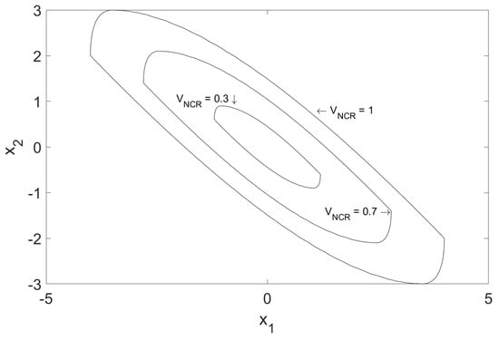
Figure 1. Level sets created using the boundary of the NCR for a MIMO linear system.

Theorem 1. 

For the dynamical system of Equation (2), with the CCLF defined by Equation (7) $\exists u\left(t\right)\in U,s.t.,{lim}_{t\to \infty }x\left(t\right)=0iff{V}_{NCR}\left(x\right)<1.$

Proof. 

The proof of the theorem follows from construction of $\partial X_{\alpha }^{max}$ in Equation (6). Noting that the NCR of the Muli-input system is the Minkowski sum of the NCR for the single input systems, $V_{NCR}\left(x\right)<1$ iff $x\in X^{max}$. Existence of $u\left(t\right)\in U,s.t.,{lim}_{t\to \infty }x\left(t\right)=0$ follows from the definition of the NCR. □

Remark 1. 

Theorem 1 formalizes two properties—one simply re-invokes the existing result that the Minkowski sum of the NCRs of the individual subsystems is the NCR of the multi-input system. The other, more pertinent result, is to establish a mapping from the level sets of the NCR of the multi-input system to the level sets of the individual subsystems. Note that the mapping from the level sets of the individual subsystems to the level sets of the multi-input system is many to one. In other words, two level sets from the individual subsystems map to a unique level set for the multi-input system, but one level set from the multi-input system maps to multiple possible combinations of level sets of the individual subsystems. Our particular choice of the level sets of the NCR, as defined by Theorem 1 as the level sets of the CCLF for the multi-input NCR, has important implications for the control design presented next.

The predictive controller that guarantees stabilization from all initial states within the NCR takes the form:

$$\begin{array}{cc}\hfill u& =argmin\{J(\overline{x},\tau ,u(·))\mid u(·)\in U,\overline{x}\left(0\right)=x\left(t\right)\}\hfill \end{array}$$

(8)

$$\begin{array}{cc}\hfill & s.t.\frac{d\overline{x}}{d\tau }=A\overline{x}+Bu\hfill \end{array}$$

(9)

$$\begin{array}{cc}\hfill & \frac{d\left(V_{NCR}\left(\overline{x}\right)\right)}{d\tau }{|}_0<0\hfill \end{array}$$

(10)

$$\begin{array}{cc}\hfill & J(x,\tau ,u(·))=q\frac{d(V_{NCR}\left(\overline{x}\left(0\right)\right)}{d\tau }+{\parallel \Delta u(\tau )\parallel }_R^2\hfill \end{array}$$

(11)

where Equation (9) is the time evolution of the process, and $V_{NCR}$ is the CCLF defined in Equation (7), q is a positive scalar and R is a positive semi-definite symmetric matrix of weightings which penalize the rate of change in inputs. The MPC calculations are done using a dummy state $\overline{x}$ which is initialized at the current value of the process state. The basic idea of the control design is to force the trajectory of the states to lower level sets, as defined by V, while still adhering to the imposed input constraints. Note that the above is a representative continuous time formulation of the MPC with the feasibility and stability properties characterized in Theorem 2. The simulation example presented later uses a discrete implementation and thus Equation (10) is implemented as $V_{NCR}(x(t+\Delta )<V_{NCR}\left(x\left(t\right)\right)$.

Theorem 2. 

Consider the MIMO System described by Equation (2) under the MPC formulation in Equations (8)–(11). For any $V\left(x_0\right)<1$, the optimization problem is feasible for all times and ${lim}_{t\to \infty }x\left(t\right)=0$.

Proof. 

The proof of the theorem follows from construction for a single input system as shown in Theorem 2 in [14] but with one critical adjustment as detailed below:

For single input systems it has been established in [14] that $\forall x_0\in X^{max}$, i.e., $\forall x_{0}s.t.V\left(x_0\right)<1,\exists u\in Us.t.\dot{V}(x_0,t,u(·))\le 0$ there are $x_0$ in $X^{max}$ for which ${min}_u\dot{V}(x_0,t,u(·))=0$. This occurs for all points given by $x\in {\epsilon }_{u_i}$ where ${\epsilon }_{u_i}=\{x:x=A^{-1}B{u}_i,u\in U\}$—additionally when $Ax$ is co-linear with $b_i$. With the assumption that the multi-input system is defined by independent inputs (i.e, all $b_i$ are linearly independent), the set ${\epsilon }_u=\{x:x=A^{-1}B{u}_i\forall i=1\cdots m\}=\mathbf{0}$. Thus, in contrast to [14], the constraint of Equation (10) is feasible for all $x\in X^{max}$, ${lim}_{t\to \infty }x\left(t\right)=0$ follows. □

Remark 2. 

The present manuscript uses the individual NCRs to construct the NCR of the multi-input system, and then directly uses the boundary of the ‘level sets’ of this NCR to define the CCLF. For single input systems, the NCR and the associated level sets have a direct relationship with the bound on the manipulated input. Thus, for the single-input system, $V_{NCR}\left(x\right)$ is the value of input constraint for which x resides on the boundary of the NCR of the single-input system with the bound $V_{NCR}\left(x\right)$. For multiple-input systems, the interpretation is that $V_{NCR}\left(x\right)$ is the value of input constraint for all the subsystems $i=1\cdots n$, for which $x_i,i=1\cdots n$ resides on the boundary of the NCR for each of the single-input systems with the bound $V_{NCR}\left(x\right)$and$x=x_1+x_2+,\cdots ,x_n$. This choice of the definition for the CCLF is fairly simple and intuitive, but, as it turns out, also non-unique (see Remark 3). This, in turn, results in a non-unique solution to the optimization problem as well, but yet, results in the stabilization for the closed-loop system. This non-uniqueness is not due to the formulation of the CCLF, but rather fundamental to the problem at hand (see Remark 4 for further explanation)

Remark 3. 

Another possible way to define a CCLF for the multiple-input system and design the controller would be to work with the individual subsystems. Thus, for the current state, the state would be projected onto each individual subsystem to find $x_i,i=1,\cdots ,n$ s.t., $x=x_1+x_2+,\cdots ,x_n$. Using each of the $x_i$, the level set of the Lyapunov function for the individual subsystems could be calculated, and the CCLF, for instance, could be defined as the sum of the CCLFs for the individual subsystem. While such a line of thinking would follow from a direct generalization of the NCR design for single-input systems, the implementation would be computationally expensive, and not alleviate the non-uniqueness issue since a state could be projected into the individual subsystems in non-unique fashion, i.e., different combinations of $x_i$ could correspond to the same state of the system. This non-uniqueness may result in jumpy control actions as new projections are evaluated at subsequent time points and due to the single-input system’s originally non-smooth input profiles [14].

Remark 4. 

By the very nature of the problem, smaller ‘level sets’ of the multi-input NCR correspond to non-unique combinations of the individual NCRs of the individual subsystems, hence multiple solutions exist that enable ${\dot{V}}_{NCR}<0$. This is simply due to the linear nature of the simple dynamics, and not due to particular choice of the NCR. The ability to guarantee and invoke the fact that ${\dot{V}}_{NCR}<0$ is achievable (not invoked in [14]), means that it can be imposed as a constraint in the optimization problem to take care of stability, leaving the objective function available as a tuning parameter to achieve a smooth control action, as is demonstrated in the simulation example.

4. Simulation Results

Five simulation trials arre performed under the MPC formulation described by Equations (8)–(11). First, a quadratic Lyapunov function $V_Q$ is set with $V_Q=x^{T}x$, $q=1$ and $R=\left[\begin{array}{cc}0& 0\\ 0& 0\end{array}\right]$. To show the stability properties of the controller under $V_Q$, two simulations are run from the initial conditions $x_0=\left[\begin{array}{c}2\\ -0.9\end{array}\right]$ and $x_0=\left[\begin{array}{c}2.5\\ -1.1\end{array}\right]$ respectively. The proposed controller design using $V_{NCR}$ is then simulated three times. To replicate the behavior of the control design in [14],with no rate of change input penalty, the controller is run with $q=1$ and $R=\left[\begin{array}{cc}0& 0\\ 0& 0\end{array}\right]$. To demonstrate the input smoothing properties of the proposed design, the second trial is shown with $q=10.2$ and $R=\left[\begin{array}{cc}0.82& 0\\ 0& 0.82\end{array}\right]$. Finally, the third trial is run with $q=10.2$ and $R=\left[\begin{array}{cc}0.82& 0\\ 0& 0.82\end{array}\right]$, from an initial condition of $x_0=\left[\begin{array}{c}-3.5\\ 2.5\end{array}\right]$ to show the stability properties of the proposed controller from additional points. The simulation example is solved using a discretization time of $\delta =0.1$ and a prediction horizon of N = 1. The optimization problem is solved using the MATLAB function FMINCON.

From an initial condition of $x_0=\left[\begin{array}{c}2\\ -0.9\end{array}\right]$, the predictive controller is implemented with $V_Q$ to stabilize the system. As shown by the light red line in Figure 2, closed-loop stability is achieved. Moving further away from the origin to an initial condition of $x_0=\left[\begin{array}{c}2.5\\ -1.1\end{array}\right]$, the controller fails to achieve stability under $V_Q$. The red lines in Figure 3a,b and Figure 4a,b show the state trajectories and input profiles of this outcome.

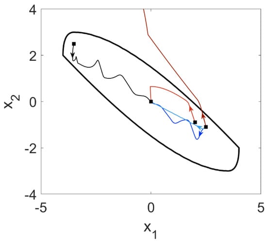
Figure 2. Evolution of the state trajectory of the multiple input multiple output liner system under various choices of the Lyapunov function. $V=V_Q$ with $q=1$ and $R=\left[\begin{array}{cc}0& 0\\ 0& 0\end{array}\right]$ from an initial condition of $x_0=\left[\begin{array}{c}2\\ -0.9\end{array}\right]$ (light red) and from an initial condition $x_0=\left[\begin{array}{c}2.5\\ -1.1\end{array}\right]$ (dark red).$V=V_{NCR}$ with $q=1$ and $R=\left[\begin{array}{cc}0& 0\\ 0& 0\end{array}\right]$ (light blue) and with $q=10.2$ and $R=\left[\begin{array}{cc}0.82& 0\\ 0& 0.82\end{array}\right]$ (dark blue). Laslty, $V=V_{NCR}$ with $q=10.2$ and $R=\left[\begin{array}{cc}0.82& 0\\ 0& 0.82\end{array}\right]$ from an initial condition of $x_0=\left[\begin{array}{c}-3.5\\ 2.5\end{array}\right]$ (black).

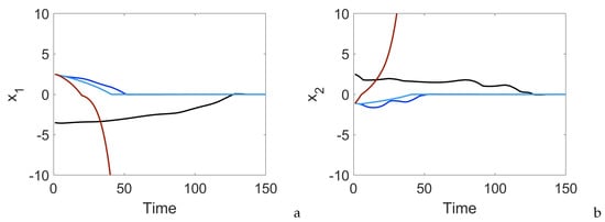
Figure 3. The system states (a,b) with $V_Q$ with an initial condition of $x_0=\left[\begin{array}{c}2.5\\ -1.1\end{array}\right]$ (red), $V_{NCR}$ for an initial condition of $x_0=\left[\begin{array}{c}2.5\\ -1.1\end{array}\right]$ with $q=1$, $R=\left[\begin{array}{cc}0& 0\\ 0& 0\end{array}\right]$(light blue), $q=10.2$ and $R=\left[\begin{array}{cc}0.82& 0\\ 0& 0.82\end{array}\right]$ (dark blue) and $V_{NCR}$ for an initial condition of $x_0=\left[\begin{array}{c}-3.5\\ 2.5\end{array}\right]$ with $q=10.2$, $R=\left[\begin{array}{cc}0.82& 0\\ 0& 0.82\end{array}\right]$(black).

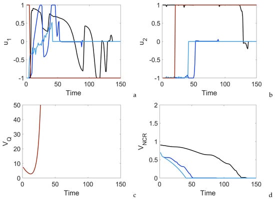
Figure 4. The system input profiles (a,b) with $V_Q$ with an initial condition of $x_0=\left[\begin{array}{c}2.5\\ -1.1\end{array}\right]$ (red), $V_{NCR}$ for an initial condition of $x_0=\left[\begin{array}{c}2.5\\ -1.1\end{array}\right]$ with $q=1$, $R=\left[\begin{array}{cc}0& 0\\ 0& 0\end{array}\right]$(light blue), $q=10.2$ and $R=\left[\begin{array}{cc}0.82& 0\\ 0& 0.82\end{array}\right]$ (dark blue) and $V_{NCR}$ for an initial condition of $x_0=\left[\begin{array}{c}-3.5\\ 2.5\end{array}\right]$ with $q=10.2$, $R=\left[\begin{array}{cc}0.82& 0\\ 0& 0.82\end{array}\right]$(black), (c) evolution of the quadratic Lyapunov function, $V_Q$ with an initial condition of $x_0=\left[\begin{array}{c}2.5\\ -1.1\end{array}\right]$ (red), (d) evolution of $V_{NCR}$ for an initial condition of $x_0=\left[\begin{array}{c}2.5\\ -1.1\end{array}\right]$ with $q=1$, $R=\left[\begin{array}{cc}0& 0\\ 0& 0\end{array}\right]$(light blue) and $q=10.2$, $R=\left[\begin{array}{cc}0.82& 0\\ 0& 0.82\end{array}\right]$ (dark blue) and $V_{NCR}$ for an initial condition of $x_0=\left[\begin{array}{c}-3.5\\ 2.5\end{array}\right]$ with $q=10.2$, $R=\left[\begin{array}{cc}0.82& 0\\ 0& 0.82\end{array}\right]$(black).

Under the proposed predictive controller and $V=V_{NCR}$ with $q=1$ and $R=\left[\begin{array}{cc}0& 0\\ 0& 0\end{array}\right]$, closed-loop stability is achieved for the initial condition $x_0=\left[\begin{array}{c}2.5\\ -1.1\end{array}\right]$. However, without the rate of change input penalty, the controller selects inputs which constantly vary, resulting in a chatty input profile, as can be seen in Figure 4a by the light blue line. Under the same initial conditions but with $q=10.2$ and $R=\left[\begin{array}{cc}0.82& 0\\ 0& 0.82\end{array}\right]$ (invoking the rate of change input penalty), the controller still achieves closed-loop stability but has a smoother input profile with fewer sporadic changes in $u_i$, as shown in Figure 4a,b (dark blue). A third initial conditional is simulated to illustrate the stability of the proposed controller with $V=V_{NCR}$, with the input and state profiles shown by the black lines in Figure 3a,b and Figure 4a–d.

Remark 5. 

The choice of q and R in this approach is made by manually tuning the controller. Note that the choice of q and R will not result in infeasibility of the optimization problem but can be used to alter the state trajectories and input profiles of the closed-loop system.

Remark 6. 

In practical applications, the proposed approach could be utilized in several ways. For instance, in deployments where a nonlinear model is available, but the controller is designed on the basis of the linearization, the proposed MPC would be applicable. In other instances, when building an empirical model from plant data, the resultant model sometimes ends up being unstable, invoking the utility of the proposed MPC. In other applications [17,18], where the MPC application is limited due to the computational complexity, the ability of the proposed MPC to achieve stability with a short horizon could be useful.

5. Conclusions and Perspectives

This manuscript addressed the problem of MPC design for MIMO linear systems subject to input constraints that is able to achieve closed-loop stability for the entire NCR without resorting to large horizon lengths. There exist several problems that can be solved in future research. In one direction, this MPC formulation could be adapted to make the controller robust to linear additive uncertainty. Further directions could be handling the output feedback problem, and/or dealing with non-symmetric input constraints, or state constraints. While these issues have been addressed in various other control designs, they have not been addressed as part of a control design that achieves stabilization from the entire NCR. Naturally, these issues represent limitations with the current formulation. The present manuscript addresses the problem of a linear system subject to symmetric input constraints. When dealing with asymmetric input constraints, the calculation of the NCR described in Section 2 is no longer valid. Results exist for the construction of the NCR for linear systems subject to non-symmetric input constraints in [19], their use for construction of the CCLF is a non-trivial problem and remains the subject of future work.

References

- Kapoor, N.; Teel, A.R.; Daoutidis, P. An Anti-Windup Design for Linear Systems with Input Saturation. Automatica 1998, 34, 559–574. [Google Scholar] [CrossRef]
- Teel, A.R. Semi-global stabilizability of linear null controllable systems with input nonlinearities. IEEE Trans. Autom. Control 1995, 40, 96–100. [Google Scholar] [CrossRef]
- Henrion, D.; Tarbouriech, S.; Kučerabc, V. Control of linear systems subject to input constraints: A polynomial approach. Automatica 2001, 37, 597–604. [Google Scholar] [CrossRef]
- Hu, T.; Lin, Z. Composite quadratic Lyapunov functions for constrained control systems. IEEE Trans. Autom. Control 2003, 48, 440–450. [Google Scholar] [CrossRef]
- Lin, Y.; Sontag, E.D. A universal formula for stabilization with bounded controls. Syst. Control Lett. 1991, 16, 393–397. [Google Scholar] [CrossRef]
- Li, Y.; Lin, Z. An asymmetric Lyapunov function for linear systems with asymmetric actuator saturation. Int. J. Robust Nonlinear Control 2018, 28, 1624–1640. [Google Scholar] [CrossRef]
- Muske, K.R.; Rawlings, J.B. Model predictive control with linear models. AIChE J. 1993, 39, 262–287. [Google Scholar] [CrossRef]
- Scokaert, P.O.M.; Rawlings, J.B. Feasibility issues in linear model predictive Control. AIChE J. 1999, 45, 1649–1659. [Google Scholar] [CrossRef]
- Grimm, G.; Messina, M.J.; Tuna, S.E.; Teel, A.R. Nominally Robust Model Predictive Control With State Constraints. IEEE Trans. Autom. Control 2007, 52, 1856–1870. [Google Scholar] [CrossRef]
- Maarouf, H. On enlarging the set of admissible initial states for the double integrator under asymmetrical constraints. Syst. Control Lett. 2019, 123, 92–97. [Google Scholar] [CrossRef]
- Li, Y.; Lin, Z.; Li, N. Stability and Performance Analysis of Saturated Systems Using an Enhanced Max Quadratic Lyapunov Function. IFAC-Pap. 2017, 50, 11847–11852. [Google Scholar] [CrossRef]
- LeMay, J. Recoverable and reachable zones for control systems with linear plants and bounded controller outputs. IEEE Trans. Autom. Control 1964, 9, 346–354. [Google Scholar] [CrossRef]
- Stephan, J.; Bodson, M.; Lehoczky, J. Calculation of recoverable sets for systems with input and state constraints. Optim. Control Appl. Methods 1998, 19, 247–269. [Google Scholar] [CrossRef]
- Mahmood, M.; Mhaskar, P. Enhanced stability regions for model predictive control of nonlinear process systems. AIChE J. 2008, 54, 1487–1498. [Google Scholar] [CrossRef]
- Homer, T.; Mhaskar, P. Constrained control Lyapunov function-based control of nonlinear systems. Syst. Control Lett. 2017, 110, 55–61. [Google Scholar] [CrossRef]
- Hu, T.; Lin, Z.; Qiu, L. An explicit description of null controllable regions of linear systems with saturating actuators. Syst. Control Lett. 2002, 47, 65–78. [Google Scholar] [CrossRef]
- Haidegger, T.; Kovács, L.; Precup, R.E.; Preitl, S.; Benyó, B.; Benyó, Z. Cascade Control for Telerobotic Systems Serving Space Medicine. IFAC Proc. Vol. 2011, 44, 3759–3764. [Google Scholar] [CrossRef]
- Li, M.; Christofides, P.D. Feedback control of HVOF thermal spray process accounting for powder size distribution. Therm. Spray Technol. 2004, 13, 108–120. [Google Scholar] [CrossRef]
- Hu, T.; Pitsillides, A.; Lin, Z. Null controllability and stabilization of linear systems subject to asymmetric actuator saturation. In Proceedings of the 39th IEEE Conference on Decision and Control (Cat. No.00CH37187), Sydney, Australia, 12–15 December 2000; Volume 4, pp. 3254–3259. [Google Scholar] [CrossRef]
Publisher’s Note: MDPI stays neutral with regard to jurisdictional claims in published maps and institutional affiliations. |
© 2021 by the authors. Licensee MDPI, Basel, Switzerland. This article is an open access article distributed under the terms and conditions of the Creative Commons Attribution (CC BY) license (https://creativecommons.org/licenses/by/4.0/).