Abstract
There is strong clinical evidence from the current literature that certain psychological and physiological indicators are closely related to mood changes. However, patients with mental illnesses who present similar behavior may be diagnosed differently, which is why a personalized study of each patient is necessary. Following previous promising results in the detection of depression, in this work, supervised machine learning (ML) algorithms were applied to classify the different states of patients diagnosed with bipolar depressive disorder (BDD). The purpose of this study was to provide relevant information to medical staff and patients’ relatives in order to help them make decisions that may lead to a better management of the disease. The information used was collected from BDD patients through wearable devices (smartwatches), daily self-reports, and medical observation at regular appointments. The variables were processed and then statistical techniques of data analysis, normalization, noise reduction, and feature selection were applied. An individual analysis of each patient was carried out. Random Forest, Decision Trees, Logistic Regression, and Support Vector Machine algorithms were applied with different configurations. The results allowed us to draw some conclusions. Random Forest achieved the most accurate classification, but none of the applied models were the best technique for all patients. Besides, the classification using only selected variables produced better results than using all available information, though the amount and source of the relevant variables differed for each patient. Finally, the smartwatch was the most relevant source of information.
1. Introduction
Personalized medicine is a new promising approach that proposes the tailoring of therapy according to the patient’s personal characteristics to ensure the best treatment outcomes. By enabling each patient to receive early (correct) diagnosis, risk assessments, and optimal treatments, personalized medicine holds promise for not only improving health care but also lowering its costs and improving patients’ quality of life [1]. This is especially true in some branches of medicine such as those dealing with mental illnesses. Indeed, there has been a large increase in the numbers of patients with mental health issues amplified by the current pandemic [2].
There is strong clinical evidence from the current literature that certain psychological and physiological indicators are closely related to mood changes [3]. However, patients with mental illnesses who present similar behavior may be diagnosed differently, which is why a personalized study of each patient is necessary. For instance, some behavioral indictors shown by patients diagnosed with bipolar depressive disorder (BDD) may be quite different from those with major depressive disorders (MDDs), being similar illnesses. BDD patients have a more complex attitude.
A current issue regarding mental health is that based solely on standard clinical inquiry (self-report and observation by a trained clinician), BDD is often misdiagnosed as unipolar depression and is treated as such. Bipolar depression patients may be treated wrongly with antidepressants for that reason, even when this therapy may aggravate their state [4,5]. However, it is possible to distinguish more than one phase in patients with BDD [6].
Therefore, in this work, supervised machine learning (ML) algorithms were applied to the classification of the different states of patients diagnosed with bipolar disorder (BD). Random Forest (RF), Decision Trees (DT), Logistic Regression (LR), and Support Vector Machine (SVM) were applied under different configurations. The final goal was to provide relevant information to medical staff and the relatives to help them deal with these situations and to make decisions on the best way to treat these patients.
The information used was collected from 17 BDD patients through wearable devices (smartwatches), daily self-reports, and medical observation at regular appointments. The variables (a total of 173) were processed and then statistical techniques for data analysis, normalization, noise reduction, and features selection were applied. An individual analysis of each patient was carried out.
The data presented in this study are available upon request from the corresponding author. Although the data have been completely anonymized and provided together with the corresponding certificate, it is not publicly available, due to the requirements of the provider, the Hospital Nuestra Señora de la Paz, in Madrid (Spain).
The results with all the variables and with only the best ranked variables by feature-selected methods were obtained and compared. Besides, some selected variables from the smartwatch were used to confirm the medical diagnosis of these patients, with good results. Moreover, adding two specific variables from the self-reporting source improved the classification. Although Random Forest gave a slightly better accuracy, none of the techniques were best for all of the patients. This result confirmed that each patient requires a personalized analysis to be able to obtain a better classification of their mood states.
The rest of the paper is structured as follows. Section 2 summarizes some related works. Section 3 details the materials used, and the machine learning techniques and methods applied. Section 4 describes the data analysis carried out, including the correlation and principal component analysis. Section 5 presents the application of some machine learning techniques to the data and discusses the results of the models. The paper ends with conclusions and future work.
2. Previous Studies
Disease diagnosis and prediction using health databases have always been a potential application area for machine learning methods [7]. They are usually applied to public databases of patients or to historical medical data collected by a certain healthcare institution. They have been used for different diseases, from cancer diagnosis [8,9,10] to diabetes [11,12].
According to [13], the Support Vector Machine (SVM) algorithm is applied most frequently, followed by the Naïve Bayes algorithm and Random Forest (RF) algorithm, the latter of which usually shows superior accuracy comparatively. Nevertheless, the application of these machine learning techniques to identify mental illnesses is not so frequent, due to the difficulty of collecting data from these patients [14]. Cho et al. [15] found that, based on a literature review, SVM, Gradient Boosting Machine (GBM), RF, Naïve Bayes, and K-Nearest Neighborhood (KNN) are the most frequently employed in the mental health area. However, they stated that, though every ML algorithm has its own advantages, researchers should be aware of the limitations of the results obtained under restricted data conditions in the practice of mental health. In the survey by Thieme [16], the authors reflected on the current state-of-the-art of ML work for mental health, and they suggested more consideration of the potential implications that ML models can have in real-world mental health contexts, as proved by other works [17].
In Costello et al. [18], an extended version of the conventional Tree-Augmented Naive Bayesian Network was applied to find the main causes leading to depression in Korea. The goal of this proposal was to help healthcare decision-makers comprehend changes in depression status. The same database was used in [19], to estimate factors affecting depression using deep learning and machine learning algorithms.
Particularly, bipolar disorder has always been considered especially difficult to diagnose accurately, as stated by Phillips and Kupfer [20]. In [21], a review of the existing literature on the use of machine learning techniques in the assessment of subjects with bipolar disorder was presented. They concluded that, given the clinical heterogeneity of samples of patients with BD, machine learning techniques may provide clinicians and researchers with important insights in fields such as diagnosis, personalized treatment, and prognosis orientation. In a more recent literature review, some advice for the proper applications of ML techniques to BDD was provided [22]. Highlighting the paramount goal of identifying etiological markers of MDD in order to help the prevention and treatment of these patients, in [23], a systematic review was conducted of all published studies reporting on the prospective relationship between positive and negative emotionality and the longitudinal course of MDD in diagnosed adults. The authors concluded that emotions are promising predictors of MDD course. In a similar way, Lima et al. [24] carried out medical research on cognitive deficits in bipolar patients. They focused on two key predictors: cognition and emotionality. They provided evidence that problems in cognition and emotionality are prominent among those diagnosed with bipolar disorder.
Regarding the sources of information for the detection of BP, they may be very different. For instance, [25] used a purpose-built online mental health questionnaire and dried blood spot samples for biomarker analysis from nine individuals with depressive symptoms. Extreme Gradient Boosting and nested cross-validation were used to train and validate diagnostic models. In [26], the design of a sensor based on physiological predictors for the continuous and autonomous monitoring of bipolar patients was proposed. It uses a pulse rate sensor to record heart rate, and an electrodermal activity sensor to trace the emotional and cognitive state changes. The extracted features from the data were then used to build machine learning models to predict the given psychological change in response to the emotional stimuli. In [27], the authors reviewed some papers on classification models applied to electroencephalographic recordings of patients with a depression diagnosis. In [28], BDD patients’ data collected from different sources were analyzed. The results showed that data from sleep and daily activity, measured both by movement and sounds, are relevant for improving the prediction of crises in patients with bipolar disorder.
In the paper by M’Bailara et al. [29], the authors used self-completed questionnaires, showing that normothymic bipolar patients displayed higher levels of emotional lability and intensity than the controls did. They carried out an emotional induction experiment based on the viewing of a set of some positive, negative, and neutral pictures. They then analyzed the reaction of normothymic bipolar patients and compared them with the control group.
In [30], the authors explored speech analysis based on phone recordings collected for the detection of mood in individuals with BDD. They classified every call into the following groups: mania/euthymic or depressive/euthymic, by applying SVM. They also proved that data preprocessing, feature extraction, and data modeling improve significantly the classifier performance. Similarly, in [31], the dynamic analysis of data from voice monitoring with accelerometers was proved to be an adequate complement to other kinds of data for predicting crises in BDD patients with a combination of machine learning algorithms.
There has been an increasing interest in using mobile sensing technologies for mental health monitoring. The use of the mobile phone was analyzed in Faurholt-Jepsen et al., [32]. In this paper, the authors claimed that objective smartphone data reflecting behavioral activities allow the classification of patients with bipolar disorder compared with healthy individuals. The results showed that the number of text messages/day and the duration of phone calls/day were increased in patients with bipolar disorder. In a similar way, Antosik-Wójcińska et al. [33] concluded that objective data automatically collected using smartphones (voice and smartphone-usage data) are valid markers of a mood state.
However, in mental health, despite the numerous mobile applications available, there are few smartwatch solutions on the market. By contrast, smartwatches, which are small and unobtrusive, and can collect data continuously, are able to monitor users’ activities and detect behavioral patterns [34]. Nevertheless, the use of wearable technology for people diagnosed with bipolar disorder and, potentially, other affective disorders, is growing [35]. As an example, in [36], contextual and sensor data were collected using smartphone and smartwatch sensors under free-living conditions. Personalized models for detecting emotional transitions and states were built using a wide range of supervised ML algorithms.
New lines of research are arising regarding this topic. For instance, the paper by Perri et al. [37] linked the disruptions in structural, functional, and effective connectivity that have been documented in BD with the impact on circuits that support emotional processes, cognitive control, and executive functions. That is, those at high risk for BD show patterns of connectivity that differ from both matched control populations, so it is possible to define those neurobiological markers.
3. Materials and Methods
One of the main contributions of this article is the analysis of both objective and subjective variables related to BDD patients. This section starts with a brief description of this mental illness to better understand some relevant indicators and variables. The database consisted of real data collected during the Bip4Cast project [31]. For this research, a proper approval of the local Ethic committee was obtained, as well as a written informed consent from all the participants. Different indicators of 17 patients diagnosed with BDD were taken from three sources: daily forms (daily self-reports filled out by the patient via a mobile app), smartwatch measurements, and clinical interviews (173 in total). Although the previous Bip4Cast research analyzed a similar dataset, further data processing is necessary in order to differentiate the specific characteristics of each patient. Indeed, in [38], it has been shown that personalized analysis is 30% more accurate than generic models.
Based on [6], four types of Bipolar Depression Disorder were identified:
- Bipolar Disorder I, characterized by depressed episodes, frequent manic episodes, or mixed episodes;
- Bipolar Disorder II, typified by full depressed and hypomanic episodes;
- Cyclothymic Disorder or Cyclothymia. It is a chronically unstable mood state in which people experience hypomania and moderate depressive episodes for at least two years;
- Unspecified Bipolar Disorder, when a patient does not meet any of the above criteria but has experienced periods of clinically significant abnormal mood elevation.
Based on these types of BDD disorders, the psychiatrist diagnoses the situation of the patient corresponding to one of the following states: Depressed, Hypomanic, Manic, or Mixed. Clinically, a crisis is defined as the appearance of one of those states. The absence of any of them is a state known as Euthymic (i.e., the patient does not suffer from any crisis). In this study, the variable “diagnosis” takes one of these 5 states (Depressed, Hypomanic, Manic, Mixed, or Euthymic). These states can be described according to clinical indicators, mood changes, or phases of the disease already described in clinical practice. The clinician modifies the diagnosis (or state), after observing significant symptoms that characterize a different new state. Figure 1, elaborated by the authors, shows the general state transitions: the nodes are the five main BDD states plus 4 more nodes for intermediate states (ED, DE, EM, and ME). The arrows show the transition between states.
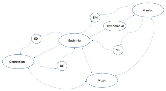
Figure 1.
Transitional state-directed graph illustrating bipolar disorder phases (nodes represent the states and arrows represent the transition).
3.1. Model Fundamentals
A patient P is characterized by a set of variables, X1, ..., Xn, where some are more explanatory than others regarding the patient’s emotional state. The value of these variables determines the mood state of the patient. However, many of these variables are correlated and, therefore, one of the first steps in the processing of the information is to determine the minimum set of variables that best represents the patient’s state.
The formalization of the Algorithm 1 that characterizes each patient is as follows.
| Algorithm 1 Characterization Algorithm |
| 1: Initialization. Let C be the set of candidate variables to be part of the patient characterization, and let W be the characterization set. Initially, vector C = {X1, ...,Xn} contains all possible variables collected, and W = Ø (empty set). The vector CV = /sx that represents the variation in the variables is calculated as the quotient between the mean and the standard deviation of each variable. |
| The correlation matrix between these variables, , X = xi ∧ Y = xj, is obtained. |
| The parameter Max: = Max(P) is the maximum number of variables for each patient P. This number will be used as Halting criteria. |
| 2: First selection. The variable Xk ∈ C = {X1, ..., Xn} with the highest CV value (variation) is selected (Initial Criterion). Then, W1 (the winner 1) is updated as W1= Xk and W: = {W1}. Remove Xk from the candidates’ set: C: = C\{W1}. The index is updated, i: = 1. |
| 3: General selection. Select the variable Xk with the lowest correlation of the set of winners W; in case of a tie, select the one with the highest variation coefficient (General Criterion). That is:
|
| 4: Update the characterization set Wi + 1: = Xk; W: = W ∪ {Wi + 1}, C: = C\W; i: = i + 1; |
| 5: Halting criterion. If |W| < Max (or another Halting criterion is met), stop. Otherwise, go to Step 2. |
After executing the Characterization Algorithm for all patients, a winner variable set W(P) = {W1, …, Wp} is obtained for patient P. This is the set of variables that characterizes the mood state of that patient. The algorithm can use any feature selection procedure. For the Halting criterion, we have used principal component analysis (PCA), in order to obtain the number of loops the algorithm must perform. This way, we try to cover 99% of the variance.
In addition, as the variables come from different sources, an integration of all the variables is necessary. For instance, the variables from the daily report are taken every 24 h. However, the variables from the accelerometer (smartwatch) are measured every 5 min. Other values of variables are obtained only when the patient goes to the doctor’s appointment. In this work, we have considered the day as the sample time unit, so the final dataset has m observations that correspond to days of the patient’s monitoring.
A patient dataset consists of an m × (p + 2) matrix where the first column represents the day, the last column contains the diagnosis of the patient (target), and the rest of the columns are the variables Wj at ti recording date.
There are more than 365 observations available for each patient, taken in a time period from October 2017 to January 2019. The monitoring time interval of a patient t1, ..., tm, is divided into slots that correspond to the different emotional states, di (Figure 1). Thus, state(P, ti1, …, tim, di) is a submatrix of dataset (P),
Machine learning methods were applied to these sub-matrices, after initial cleaning and other processing operations explained in the following sections.
3.2. Data Collection
The Bip4Cast data came from a study carried out in collaboration with a public hospital, Nuestra Sra. de la Paz (Madrid, Spain). The BDD patients were evaluated and diagnosed by an experienced psychiatrist. All of the patients satisfied both ICD-11 (International Classification of Diseases. 11th Revision) and DSM-5 (Diagnostic and Statistical Manual of Mental Disorders, Fifth Edition) criteria.
The variables were collected from different information sources:
- Smartwatches/bands. Each patient has their own medical smart band. This device gathers a set of objective variables (physical activity, sleep quality, etc.) and up to 110 activity variables. The actigraphy as a data source has been proved to be very useful [39].
- Fill-in forms. Patients complete an electronic form on a daily basis. This form was designed as part of the Bip4Cast project for gathering a total of 20 variables. Some of them are quantitative, e.g., coffee, tobacco, or alcohol consumption, and periods of menstruation. Others are qualitative variables such as anxiety, concentration, and comfort. When there are missing data in self-daily reports, interpolation is applied. These are subjective variables as they are directly reported by the patient.
- Periodical interviews during medical consultation. In these sessions, the psychiatrist registers a total of 40 variables. HDRS (Hamilton Depression Rating Scale) and YMRS (Young Mania Rating Scale) items are included. Patients are diagnosed more than once monthly (usually every two weeks). Therefore, the variable “diagnosis” is also collected. According to the psychiatrist, a diagnosis should be maintained until changes in the patient’s symptoms occur, that is, until the next diagnosis. The diagnosis is directly related to the HDRS and YMRS tests. This source of data consists of subjective and objective variables.
The data from these three sources have a different structure/format. Thus, data processing was necessary to integrate all this information into a single data structure. This work used the preprocessing functions offered by RStudio in the specific-use library “tidyverse” [40]. This library contains the necessary functions for information fusion from different sources and to apply some data processing such as cleaning, formatting, normalization, standardization, and interpolation.
In this project, patients used a specific smartwatch, GENEACTIV 1.1 [41] https://www.activinsights.com/technology/geneactiv/, accessed on 21 May 2021), whose accuracy has been measured [42]. We did not use any specific application other than the R language, particularly, the R CGIR library. GGIR is an R-package to process multi-day raw accelerometer data for physical activity and sleep research [43].
The new single data structure integrates 173 variables, where two of them are key variables (ID of the patient and timestamp). A record of this data structure corresponds to one day of a specific patient. The new structure is scalable and open to growing with other variables and new sources (as voice recording, images, and video).
Table 1 shows the data structure, with 6 groups of variables, and the type, source of information, and frequency of each variable. The different frequency of sampling imposes escalation of the data.

Table 1.
Data structure of all the variables.
The dataset contains diagnosis observations from 17 patients who have been monitoring with smartwatches, and who have filled the self-daily reports during a significant period (more than one month in a row). The personal information of the patients was previously anonymized. In this work, we referred to them as P01 to P17. Table 2 shows the states of the 17 patients between October 2017 and January 2019. All of them have had one or more crisis episodes within the period of observation.
Table 2.
States of the patients during the recollection period.
To better identify the source of each variable, all of them have been named by adding a character at the beginning: “S_” for smartwatches, “D_” for daily forms (self-daily reports), “I_” for interviews, “H” for HRDS scale, and “Y_” for Young scale. Although the same variables have been collected for all patients, according to the characteristics of each one, only some of them will be relevant for each particular patient. For example, the variable tobacco does not provide any useful information about a nonsmoking patient.
To obtain the relevant variables for a specific patient, 8 Feature Selection (FS) methods were applied (A–H in Table 3): Boruta from Random Forest algorithm (A), Variable Importance from machine learning algorithms (B), LASSO (Least Absolute Shrinkage and Selection Operator) (C), STEPWISE (D), Recursive Feature Elimination (E), Genetic Algorithm (F), Simulated Annealing (G), and Descriptive Machine Learning Explanation (DALEX) (H).
Table 3.
Selected variables by the Feature Selection methods for patient P07.
Each of those FS algorithms returns a list of variables that have more impact in order to analyze the target variable (diagnosis). However, not all FS procedures gave the same group of variables. For this reason, we ranked each variable by the number of FS procedures that returned it. Table 3 shows, as an example, the top 10 ranked variables for patient P07.
As it is possible to see in Table 3, the 10 first variables of patient P07 were selected by at least 4 different methods. The smartwatch was the most relevant source of information in all cases (7 out of 10 in the list). Nevertheless, the amount and nature of the relevant variables differed for each patient.
3.3. Classification Methods
Different machine learning (ML) algorithms were applied to classify the observations. Random Forest (RF), Decision Trees (DT), Logistic Regression (LR), and Support Vector Machine (SVM) were used under different configurations. The code has been written in R language with RStudio. Table 4 shows the algorithms and the specific libraries applied in this study.
Table 4.
Machine learning algorithms and the corresponding R libraries.
A brief description of each ML technique that was applied is given below.
Decision Tree (DT) is an algorithm that predicts values of responses by learning the decision rules derived from the features. There are different ways to construct decision trees; the one used here was the Classification and Regression Trees (CART). This is a supervised learning technique where there is a target variable (which is dependent) and the goal is to obtain a function that procures the value of the target variable for unknown cases, from predictor variables (which are independent). The particular implementation of CART we used was Recursive Partitioning and Regression Trees (RPART).
Random Forest (RF) is an algorithm that uses supervised training. It builds individual decision trees for training. Predictions from all the trees are aggregated to achieve one final prediction. The algorithm randomly selects a certain number of columns and rows from entire data for building a decision tree from them. This process is repeated many times and different trees are built. The higher the number of trees constructed, the smaller the classification errors.
Support Vector Machine (SVM) is a supervised algorithm used for classification and regression problems. The main idea of SVM is to separate classes with a straight line (1 dimension), flat plane (2 dimensions), or an N-dimensional hyperplane. SVM uses kernel (nonlinear) functions to separate classes when it is necessary according to the data. SVM finds the best hyperplane by defining a decision boundary with the margin between the groups as large as possible.
Logistic regression (LG) is a regression model (also known as logit regression) for estimating the parameters of a logistic model, a binary model that has a dependent variable with two possible values, usually 0 and 1. In this model, the logarithm of the odds (or 1) is a linear combination of the independent (predictors) variables. In the logistic regression model, the dependent variable is a logistic function (Equation (1)). This function varies between (0, 1) for an input Y in (−∞, +∞) and, thus, the logistic function is ideal for modeling any binary response. The inverse of the logistic function is logit (Equation (2)). In logistic regression, the variable Y is treated as a linear function of a vector variable . That is, the logistic regression model can be defined as Equation (3).
Detailed information of these algorithms and applications can be found in [44].
4. Data Analysis
This section describes the kind of personalized analysis applied to each patient’s data. First, the correlation obtained between the variables is presented and the necessity to reduce dimensionality is justified. Then, principal component analysis (PCA) is carried out and the results are discussed.
4.1. Correlation Analysis
The first step of the data analysis was to determine the correlation between the variables for each individual patient. The different degrees of correlation justified the feature selection process that was carried out as a second step. In this article, patient P07 has been selected as an illustration for the results obtained.
Figure 2 shows the correlation matrix of the first 15 ranked variables obtained for patient P07 from the feature selection procedures. The colour code is red, maximum value of correlation; white, minimum correlation; reddish, positive correlation; bluish, negative correlation. The results showed some highly dependent variables, such as variables related to nighttime activity (S_dur_spt_wake_LIG_min, S_Nblocks_spt_wake_MOD and S_Nblocks_spt_wake_LIG). It can also be concluded that this patient (P07) engaged in light and moderate physical activities in the nights of recordings. The high correlation (0.83) between D_sleep_zenith and D_wakeup_time means that, regardless of the time patient P07 fell asleep, the number of sleeping hours was almost the same every day.
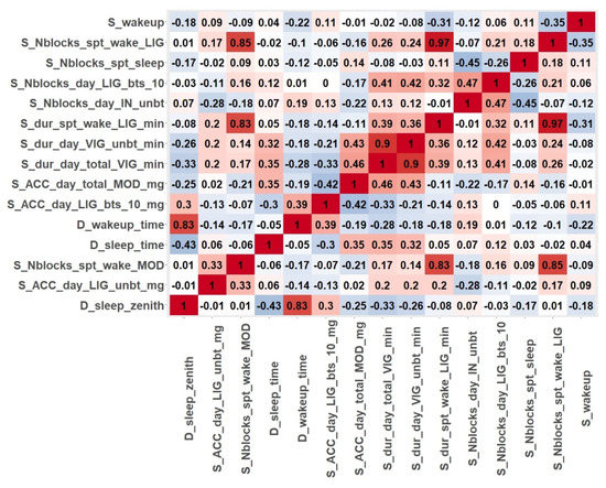
Figure 2.
Correlation matrix for the features selected for patient P07.
The study of the correlation between variables together with the large number of variables of the original dataset clearly justified the need for reducing the dimensionality of the problem.
In addition to the correlation among features, some specific variables were further analyzed. In Figure 3, some variables from patient P07′s data are represented, and some interesting insights can be drawn. For example, Figure 3a shows that P07 tended to sleep better in the euthymic state, and according to Figure 3b, this patient engaged in less light physical activity when in the depressed state. In Figure 3c, it is shown that patient P07 usually woke up more often in the euthymic state than in any other state. Figure 3d shows that this patient fell asleep earlier in the euthymic state than in any other case. In Figure 3e, it is possible to observe that the level of vigorous physical activity was unstable when depressed. Finally, Figure 3f allows us to conclude that patient P07 engaged in the same light physical activity in the sleep period times in any state. This information can help to establish some rules to predict the state of each particular individual.
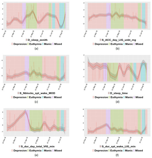
Figure 3.
Graphical representation of some variables of patient P07: (a) sleep zenith; (b) acceleration in light state; (c) times of waking up in moderate state; (d) time to go to rest; (e) time spent in vigorous state; (f) time spent in light state in sleep period time.
The correlation coefficient was also calculated for all variables with the target variable (diagnosis) for every patient. Table 5 shows some of the variables for only those patients whose correlation coefficient was greater than 0.5 or lower than −0.5.
Table 5.
Variables with the highest correlation with variable diagnosis for some patients.
It is possible to see in Table 5 that the most correlated variables with the diagnosis were those that belong to HRSD and Young scales, as expected. They are directly related with the diagnosis itself and the specialists use them to diagnosis the patient.
4.2. Principal Component Analysis
Principal component analysis (PCA) is a statistical technique that is applied to reduce the dimension of a dataset. It finds the components that define the basic structure of the dataset. In our case, the nonnumeric variables were removed before applying PCA. In addition, NA values were interpolated, and the complete dataset was normalized.
The PCA procedure results in a list of variables (“principal components”-PCx) that covers the variance of the original dataset. The list is sorted by the level of variance covered. That is, the first components cover the majority of the variance of the original dataset. Figure 4 shows, as an example, the covered variance: (a) relative and (b) cumulative, of the patient P05 dataset. It is possible to see how the first three principal components covered together more than 95% of the variance, and the first seven covered more than 99%. That means that the dimensionality of the study for patient P05 could be reduced to seven variables.
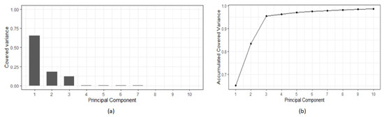
Figure 4.
Principal component analysis results of patient P05 data: (a) Covered variance; (b) accumulated variance.
4.3. General Settings and Configuration of the ML Techniques
Supervised ML algorithms were applied to the available data. The dataset was split into training and testing datasets. The training set consisted of 70% observations randomly selected, and the testing data consisted of the 30% remaining observations. Several mathematical models were obtained using the diagnosis as the target variable. The accuracy of these models was calculated through the confusion matrix. The accuracy was calculated by adding all the values in the diagonal of the confusion matrix and dividing the result by the total number of observations.
The code used to generate each model and the configuration of each ML method are shown in Table 6. For SVM, a classification machine was used; thus, “type parameters” is “C-classification,” with a linear kernel. Random Forest used 500 as the number of trees to grow, and the minimum size of the nodes for classification was one. The “method” selected for the Decision Trees technique was “class,” to perform a classification. The default parameter method of Logistic Regression was “glm.fit,” which uses iteratively weighted least squares (IWLS). The “family parameter” was binomial. The binomial family accepts different links such as logit, probit, and cauchit, which correspond to logistic, normal, and Cauchy CDFs, respectively.
Table 6.
Parametrization used for the generation of machine learning models.
5. Results and Discussion
The application of ML techniques was intended to help confirm the diagnosis of the psychiatrist. ML methods acquire the diagnosis based on learning from collected variables automatically. All the techniques applied performed a supervised classification process, and, thus, they assigned a new observation to a specific mood state. First, the four selected ML techniques were applied to all the variables. Table 7 shows the obtained percentage of accuracy of each model for some of the patients.
Table 7.
Accuracy (%) of every ML model obtained with all the variables for some of the patients.
From Table 7, it is possible to conclude that, though Random Forest gave the best results, for some patients (P06, P16), other techniques worked better. This means that none of the algorithms were best for all patients. Selecting a specific one for each patient gave the best results.
The same ML techniques were applied to the variables selected by the feature selection algorithms. Variables whose rank was over 3 were used, i.e., those that were selected by at least three FS procedures. Table 8 shows the obtained percentage of accuracy of each model for the same patients of Table 7.
Table 8.
Accuracy (%) of every ML model obtained with only the feature-selected variables.
The results from Table 8 show that using feature selection before applying machine learning techniques, in almost all cases, provided better results than using all the variables for classification, without selecting the most relevant ones.
Comparing the results with previous studies on a similar dataset, in [28], the best algorithm in terms of accuracy was Random Forest (mean of 72%). The present work reached a higher accuracy, with an average of 80% with that technique. The main improvement was due to the addition of objective variables (smartwatch variables) and by the application of feature selection algorithms prior to classification.
Finally, the classification results using only three smartwatch variables (Table 9) and adding two variables from the self-daily report (Table 10) were obtained for comparison purposes. These accelerometer variables were control sleep time, wake-up time, and daytime activity; the chosen self-report variables were irritability and motivation.
Table 9.
Accuracy (%) of the classification of mood states based on 3 selected smartwatch variables.
Table 10.
Accuracy (%) of the classification of mood states based on 3 smartwatch variables and 2 daily form variables preselected.
From Table 9 and Table 10, it can be observed that in 80% of the cases, the classification improved when the variables of the daily self-report were added. The best model was, most prominently, RF. The best-classified cases corresponded to patients with two states (Euthymia-Mixed and Euthymia-Mania) or three states (Euthymia-Mania-Depression). The worse results could have been a consequence of the lack of collaboration of the patients in completing the daily self-report (such as reporting inaccurate information about their present state). It is also shown that some of the patients collaborated when they were in the euthymic state only (that is, in absence of any crisis). This was another limitation of such a methodology pipeline and should be considered in the interpretation of the results.
6. Conclusions and Future Work
This study has allowed us to gain another perspective of ML application to detect BDD states from relevant factors extracted from both objective and subjective data, which can facilitate future patients’ treatments. Currently, there are many people who suffer from this mental illness, which also affects their immediate environment and their skills in ordinary life.
In this work, heterogeneous sources of information have been combined. Data from patients diagnosed with BDD have been obtained through smartwatches, questionnaires, and standard medical consultations with the specialist. Several ML techniques have been applied with different configurations to classify the different states present in BDD patients, and to validate the most relevant factors for future detection.
The present results, regardless of the level of accuracy in successfully confirmed diagnosis, have allowed us to draw the following conclusions.
- The study required the active participation of the patients to collect the data from at least two sources of information. However, it was found that the information given by some of the patients in self-reports are sometimes not reliable, especially when the patient is in a specific mood state (mania). In this sense, the people who live with or take care of them can have a crucial role in objectifying some of the factors that they are asked about in the questionnaires.
- Many BDD patients do not use smartwatches frequently, despite being nonintrusive devices. They forget to put them on at times when it is important to collect information (sleep and activity). Again, relatives or caregivers can help to remind them to wear those devices.
- There are some patients who actively participate (reporting accurate data) when they are in a state of euthymia only.
- The analysis of the data of each patient must be carried out individually, and it is only possible to compare and detect the changes in mood state in relation to each person. This is due to the fact that each patient manifests different levels of intensity of the symptoms that correspond to a particular emotional state. In addition, the manifestations of a certain state can change for a specific patient over time as a consequence of the changing nature of this illness.
- It is difficult to obtain the data from patients that are monitored and followed by a specialist, hence the low number of samples in the databases of this type of patient, and in general, of all those suffering from mental illness.
Regarding the methods and the results, a reduced set of smartwatch variables have been proven to be good enough to obtain good results in the classification of the different states of the disease. Furthermore, these results are improved when reliable information provided by the patient via self-reports are available.
This study confirms that a simple, low-cost, and nonintrusive device could help to assess the correct diagnosis for BDD and to relate symptoms with different mood changes in a feasible way. In order to acquire a deeper understanding of this mental disorder with very complex dynamics, much larger datasets are necessary.
Therefore, further works include acquiring larger datasets, and to apply this methodology to patients with other psychiatric disorders. Besides, inspired by [7,45,46], other classification methods, e.g., the C4.5 classification algorithm or neural network, could be tested on the dataset. This will allow us to design a computational tool for health decision making.
Author Contributions
Conceptualization, V.L and M.S.; methodology, V.L. software, P.L.; validation, P.L., V.L., M.S. and M.Č.; formal analysis, V.L.; investigation, P.L.; writing—original draft preparation, P.L. and V.L.; writing—review and editing, M.S. and M.Č.; supervision, M.S. and M.Č.; funding acquisition, V.L. All authors have read and agreed to the published version of the manuscript.
Funding
The APC was funded by CUNEF University, Spain.
Institutional Review Board Statement
The study was conducted in accordance with the Declaration of Helsinki, and the protocol was approved by the Ethics Committee of Project Bip4Cast Ref. A-83-4155904.
Informed Consent Statement
Informed consent was obtained from all subjects involved in the study.
Data Availability Statement
Not applicable.
Acknowledgments
The authors thank the Hospital Nuestra Sra. de la Paz (Madrid) for the data.
Conflicts of Interest
The authors declare no conflict of interest.
References
- Mathur, S.; Sutton, J. Personalized medicine could transform healthcare. Biomed. Rep. 2017, 7, 3–5. [Google Scholar] [CrossRef] [PubMed]
- Inkster, B.; Digital Mental Health Data Insights Group (DMHDIG). Early Warning Signs of a Mental Health Tsunami: A Coordinated Response to Gather Initial Data Insights from Multiple Digital Services Providers. Front. Digit Health 2021, 2, 578902. [Google Scholar] [CrossRef]
- Čukić, M.; Stokić, M.; Radenković, S.; Ljubisavljević, M.; Simić, S.; Savić, D. Nonlinear analysis of EEG complexity in episode and remission phase of recurrent depression. Int. J. Res. Methods Psychiatry 2019, 2019, e1816. [Google Scholar] [CrossRef]
- Singh, T.; Rajput, M. Missdiagnosis of Bipolar Dysorder. Psychiatry Edgmont 2006, 3, 57–63. [Google Scholar] [PubMed]
- Patel, R.; Reiss, P.; Shetty, H.; Broadbent, M.; Stewart, R.; McGuire, P.; Taylor, M. Do antidepressants increase the risk of mania and bipolar disorder in people with depression? A retrospective electronic case register cohort study. BMJ Open 2015, 5. [Google Scholar] [CrossRef]
- Murnane, E.L.; Cosley, D.; Chang, P.; Guha, S.; Frank, E.; Gay, G.; Matthews, M. Self-monitoring practices, attitudes, and needs of individuals with bipolar disorder: Implications for the design of technologies to manage mental health. J. Am. Med. Inform. Assoc. 2016, 23, 477–484. [Google Scholar] [CrossRef]
- Sahoo, A.K.; Pradhan, C.; Das, H. Performance evaluation of different machine learning methods and deep-learning based convolutional neural network for health decision making. In Nature Inspired Computing for Data Science; Springer: Cham, Switzerland, 2020; pp. 201–212. [Google Scholar]
- Farias, G.; Santos, M.; López, V. Making decisions on brain tumor diagnosis by soft computing techniques. Soft Comput. 2010, 14, 1287–1296. [Google Scholar] [CrossRef]
- Chugh, G.; Kumar, S.; Singh, N. Survey on Machine Learning and Deep Learning Applications in Breast Cancer Diagnosis. Cogn. Comput. 2021, 1–20. [Google Scholar] [CrossRef]
- Ak, M.F. A comparative analysis of breast cancer detection and diagnosis using data visualization and machine learning applications. Healthcare 2020, 8, 111. [Google Scholar] [CrossRef]
- Manrique-Cordoba, J.; Romero-Ante, J.D.; Vivas, A.; Vicente, J.M.; Sabater-Navarro, J.M. Mathematical modeling of food intake and insulin infusion in a patient with type 1 Diabetes in closed loop. Rev. Iberoam. Autom. E Inform. Ind. 2020, 17, 156–168. [Google Scholar]
- Rghioui, A.; Lloret, J.; Sendra, S.; Oumnad, A. A Smart Architecture for Diabetic Patient Monitoring Using Machine Learning Algorithms. Healthcare 2020, 8, 348. [Google Scholar] [CrossRef] [PubMed]
- Uddin, S.; Khan, A.; Hossain, M.E.; Moni, M.A. Comparing different supervised machine learning algorithms for disease prediction. BMC Med. Inform. Decis. Mak. 2019, 19, 1–16. [Google Scholar] [CrossRef] [PubMed]
- Graham, S.; Depp, C.; Lee, E.E.; Nebeker, C.; Tu, X.; Kim, H.C.; Jeste, D.V. Artificial intelligence for mental health and mental illnesses: An overview. Curr. Psychiatry Rep. 2019, 21, 1–18. [Google Scholar] [CrossRef] [PubMed]
- Cho, G.; Yim, J.; Choi, Y.; Ko, J.; Lee, S.H. Review of machine learning algorithms for diagnosing mental illness. Psychiatry Investig. 2019, 16, 262. [Google Scholar] [CrossRef]
- Thieme, A.; Belgrave, D.; Doherty, G. Machine learning in mental health: A systematic review of the HCI literature to support the development of effective and implementable ML systems. ACM Trans. Comput. Hum. Interact. Tochi 2020, 27, 1–53. [Google Scholar] [CrossRef]
- Chekroud, A.M.; Zotti, R.J.; Shehzad, Z.; Gueorguieva, R.; Johnson, M.K.; Trivedi, M.H.; Cannon, T.D.; Krystal, J.H.; Corlett, P.R. Cross-trial prediction of treatment outcome in depression: A machine learning approach. Lancet Psychiatry 2016, 3, 243–250. [Google Scholar] [CrossRef]
- Costello, F.J.; Kim, C.; Kang, C.M.; Lee, K.C. Identifying High-Risk Factors of Depression in Middle-Aged Persons with a Novel Sons and Spouses Bayesian Network Model. Healthcare 2020, 8, 562. [Google Scholar] [CrossRef] [PubMed]
- Oh, J.; Yun, K.; Maoz, U.; Kim, T.S.; Chae, J.H. Identifying depression in the National Health and Nutrition Examination Survey data using a deep learning algorithm. J. Affect. Disord. 2019, 257, 623–631. [Google Scholar] [CrossRef] [PubMed]
- Phillips, M.L.; Kupfer, D.J. Bipolar disorder diagnosis: Challenges and future directions. Lancet 2013, 381, 1663–1671. [Google Scholar] [CrossRef]
- Librenza-Garcia, D.; Kotzian, B.J.; Yang, J.; Mwangi, B.; Cao, B.; Lima, L.N.P.; Passos, I.C. The impact of machine learning techniques in the study of bipolar disorder: A systematic review. Neurosci. Biobehav. Rev. 2017, 80, 538–554. [Google Scholar] [CrossRef] [PubMed]
- Claude, L.A.; Houenou, J.; Duchesnay, E.; Favre, P. Will machine learning applied to neuroimaging in bipolar disorder help the clinician? A critical review and methodological suggestions. Bipolar Disord. 2020, 22, 334–355. [Google Scholar] [CrossRef]
- Moris, B.H.; Bylsma LMRottenberg, J. Does emotion predict the course of major depressive disorder? A review of prospective studies. Br. J. Clin. Psychol. 2009, 48, 255–273. [Google Scholar] [CrossRef]
- Lima, I.M.; Peckham, A.D.; Johnson, S.L. Cognitive deficits in bipolar disorders: Implications for emotion. Clin. Psychol. Rev. 2018, 59, 126–136. [Google Scholar] [CrossRef] [PubMed]
- Tomasik, J.; Han, S.Y.S.; Barton-Owen, G.; Mirea, D.M.; Martin-Key, N.A.; Rustogi, N.; Bahn, S. A machine learning algorithm to differentiate bipolar disorder from major depressive disorder using an online mental health questionnaire and blood biomarker data. Transl. Psychiatry 2021, 11, 1–12. [Google Scholar] [CrossRef]
- Anwar, Y. Bipolar Disorder Predictive Model: A Study to Analyze and Predict Emotional Change Using Physiological Signals. Master’s Thesis, University of Minnesota, Minneapolis, MI, USA, 2019. [Google Scholar]
- Čukić, M.; López, V.; Pavón, J. Classification of Depression through Resting-State Electroencephalogram as a Novel Practice in Psychiatry. J. Med. Internet Res. 2020, 22, e19548. [Google Scholar] [CrossRef] [PubMed]
- Llamocca Portella, P.; Čukić, M.; Junestrand, A.; Urgelés, D.; López, V.L. Data source analysis in mood disorder research. In Proceedings of the XVIII Conferencia de la Asociación Española para la Inteligencia Artificial (CAEPIA 2018), Granada, Spain, 23–26 October 2018; pp. 893–898. [Google Scholar]
- M’Bailara, K.; Demotes-Mainard, J.; Swendsen, J.; Mathieu, F.; Leboyer, M.; Henry, C. Emotional hyper-reactivity in normothymic bipolar patients. Bipolar Disord. 2009, 11, 63–69. [Google Scholar] [CrossRef] [PubMed]
- Gideon, J.; Provost, E.M.; McInnis, M. Mood State prediction from speech of varying acoustic quality for individuals with Bipolar Disorder. In Proceedings of the IEEE International Conference on Acoustics, Speech, and Signal Processing, ICASSP, Shanghai, China, 20–25 March 2016; pp. 2359–2363. [Google Scholar]
- López, V.; Valverde, G.; Anchiraico, J.C.; Urgeles, D. Specification of a Cad Prediction System for Bipolar Disorder. In Uncertainty Modelling in Knowledge Engineering and Decision Making, Proceedings of the 12th International FLINS Conference, Istanbul, Turkey, 26–29 Ausgust 2016; World Scientific: Singapore, 2016; pp. 162–167. [Google Scholar]
- Faurholt-Jepsen, M.; Busk, J.; Þórarinsdóttir, H.; Frost, M.; Bardram, J.E.; Vinberg, M.; Kessing, L.V. Objective smartphone data as a potential diagnostic marker of bipolar disorder. Aust. N. Z. J. Psyquiatry 2019, 53, 119–128. [Google Scholar] [CrossRef] [PubMed]
- Antosik-Wójcińska, A.Z.; Dominiak, M.; Chojnacka, M.; Kaczmarek-Majer, K.; Opara, K.R.; Radziszewska, W.; Święcicki, Ł. Smartphone as a monitoring tool for bipolar disorder: A systematic review including data analysis, machine learning algorithms and predictive modelling. Int. J. Med. Inform. 2020, 138, 104131. [Google Scholar] [CrossRef] [PubMed]
- Motti, V.G. Smartwatch Applications for Mental Health: A Qualitative Analysis of the Users’ Perspectives. JMIR Ment. Health 2018. [Google Scholar] [CrossRef]
- Tran, T.; Nathan-Roberts, D. Design Considerations in Wearable Technology for Patients with Bipolar Disorder. In Proceedings of the Human Factors and Ergonomics Society Annual Meeting, Philadelphia, PA, USA, 1–5 October 2018; Volume 62, pp. 1187–1191. [Google Scholar]
- Sultana, M.; Al-Jefri, M.; Lee, J. Using Machine Learning and Smartphone and Smartwatch Data to Detect Emotional States and Transitions: Exploratory Study. JMIR Mhealth Uhealth 2020, 8, e17818. [Google Scholar] [CrossRef] [PubMed]
- Perry, A.; Roberts, G.; Mitchell, P.B.; Breakspear, M. Connectomics of bipolar disorder: A critical review, and evidence for dynamic instabilities within interoceptive networks. Mol. Psychiatry 2019, 24, 1296–1318. [Google Scholar] [CrossRef]
- Constantinides, M.; Busk, J.; Matic, A.; Faurholt-Jepsen, M.; Kessing, L.V.; Bardram, J.E. Personalized versus generic mood prediction models in bipolar disorder. In Proceedings of the 2018 ACM International Joint Conference and 2018 International Symposium on Pervasive and Ubiquitous Computing and Wearable Computers, Singapore, 9–11 October 2018; pp. 1700–1707. [Google Scholar]
- Geoffroy, P.A.; Boudebesse, C.; Bellivier, F.; Lajnef, M.; Henry, C.; Leboyer, M.; Scott, J.; Etain, B. Sleep in remitted bipolar disorder: A naturalistic case-control study using actigraphy. J. Affect. Disord. 2014, 158, 1–7. [Google Scholar] [CrossRef]
- Wickham, H.; Averick, M.; Bryan, J.; Chang, W.; McGowan, L.D.A.; François, R.; Yutani, H. Welcome to the Tidyverse. J. Open Source Softw. 2019, 4, 1686. [Google Scholar] [CrossRef]
- Geneactiv. Available online: https://www.activinsights.com/technology/geneactiv/ (accessed on 20 May 2021).
- Pavey, T.G.; Gomersall, S.R.; Clark, B.K.; Brown, W.J. The validity of the GENEActiv wrist-worn accelerometer for measuring adult sedentary time in free living. J. Sci. Med. Sport 2016, 19, 395–399. [Google Scholar] [CrossRef] [PubMed]
- Migueles, J.H.; Rowlands, A.V.; Huber, F.; Sabia, S.; van Hees, V.T. GGIR: A Research Community–Driven Open Source R Package for Generating Physical Activity and Sleep Outcomes from Multi-Day Raw Accelerometer Data. J. Meas. Phys. Behav. 2019, 2. [Google Scholar] [CrossRef]
- Flach, P. Machine Learning: The Art and Science of Algorithms that Make Sense of Data; Cambridge University Press: Cambridge, UK, 2012; ISBN 9781107422223. [Google Scholar]
- Paoletti, M.E.; Haut, J.M.; Plaza, J.; Plaza, A. A Comparative study of ML techniques for hyperspectral image classification. Rev. Iberoam. Autom. E Inform. Ind. 2019, 16, 129–137. [Google Scholar] [CrossRef]
- Guevara, C.; Santos, M. Intelligent models for movement detection and physical evolution of patients with hip surgery. Log. J. Igpl. 2020, jzaa032. [Google Scholar] [CrossRef]


Publisher’s Note: MDPI stays neutral with regard to jurisdictional claims in published maps and institutional affiliations. |
© 2021 by the authors. Licensee MDPI, Basel, Switzerland. This article is an open access article distributed under the terms and conditions of the Creative Commons Attribution (CC BY) license (https://creativecommons.org/licenses/by/4.0/).