Abstract
This paper focuses on the dynamic effects of flexible propellers on F2 class aircraft models. An oscillating propeller affects an engine’s mechanical performance, and this combination has a huge influence on the model’s flight dynamic performance. In the first and second sections of this paper, two physical tests that were performed according to the test results obtained using a CFX numerical model are discussed. The studies on flexible propellers for class F2 aircraft models performed in this paper show that, when the first resonant frequencies of the propeller are within the operating range of the aircraft, better flight parameters are achieved. This study helps to explain the effect of a glass composite’s Young’s modulus on the mechanical behavior of a physical propeller in operating conditions and the effect of propeller stiffness on flapping propeller dynamics and unsteady aerodynamics.
1. Introduction
Flapping propeller phenomena have continued to be the focus of many researchers for many years due to their positive contribution to aerodynamic performance [1]. This effect can also be found in nature, such as in birds and insects, as well as in manmade apparatus, such as airplanes. Flapping phenomena could be used in the application of airplane construction elements, such as wings or propellers, to increase effectivity, power, and flight time. The propeller, from the perspective of aerodynamics, can be viewed as a spinning wing; therefore, the cause of flapping [2] is identical for the thrust generation mechanics of both wing and propeller elements.
Due to the high complexity of a flapping foil, the object of investigation can be simplified into two dimensions, as researchers investigate the lift, drag, and thrust for 2D models and compare these results with flapping profiles.
Researchers Knoller and Betz [2,3] were the first to investigate flapping foil and to explain flapping-wing thrust generation mechanics.
One of the first comprehensive investigations of a flapping wing was reported by [3], who demonstrated equations for the theoretical efficiency of flapping motion and the effect of angular oscillations.
Thrust-producing harmonically oscillating foils are studied through force and power measurements by [4]. In this research, the data were obtained using digital particle image velocimetry. The authors found that conditions of high efficiency are associated with the formation of a moderately strong vortex on alternating sides of the foil, which interacts with the leading-edge vorticity and creates a reverse Karman street.
A group of researchers, Benkherouf et al., Chen and Liu, and Xiao and Zhu [5,6,7], provided a 2D foil-flapping numerical investigation using Navier–Stokes equations-based fluid flow modeling.
Gopalkrishnan et al. and Streitlien and Triantafyllou [8,9] gave three basic types of interactions of a harmonically oscillating wing with vortices in the wake: (1) an optimal interaction of newly generated vortices, with the general vortices shed by the wing, resulting in +C in the generation of more powerful vortices in the reverse Karman vortex street; (2) a destructive interaction of new vortices with those shed by the wing, resulting in the generation of weaker vortices in the reverse Karman street; and (3) the interaction of vortex pairs with an opposite sign shed from the wing, leading to the generation of a wide wake composed of vortex pairs that are shed at an angle to the freestream.
Since then, various types of device that use a flapping-foil motion have been proposed. One possible use is demonstrated by ship propellers, as a flapping propeller foil generates thrust for the ship’s motion and propulsion [10,11,12,13].
In [14], a review of a wide flapping foil was given. The authors observed that a 2D flapping-foil investigation cannot fully explain the flapping-structure mechanics due to the complicated 3D flow patterns. In this paper, they focused on high-speed RPM airplane propellers with a relatively low k (reduced frequency): , where f indicates the frequency (Hz), c is profile length (m), and represents flow speed (m/s).
In the case of an insect’s flight, the wing-beating frequencies obtained from physical tests showed that they are significantly lower than the resonant frequencies, as shown in [15]. The dragonfly flutter frequency is about 16% of the first resonant frequency (dragonfly flapping frequency of 27 Hz is about 16% of the fundamental natural frequency). Studies of elastic wings with a large flapping amplitude in [16,17] showed that the highest efficiency was achieved when the wing-flapping frequency was lower than the first wing resonance.
These articles describe the mechanisms that control the dynamics of fluttering wings, but it is clear that the basic details of the problem of fluid–structure interaction are still poorly understood. More specifically, the basic phase dynamics, which determine the instantaneous shape of the wing and lead first to an increase in the traction force fluctuation, remains unexplained [18].
It has been reported that wing flexibility allows for flight energy consumption to be reduced [19]. For real flight conditions, simulation results show that these energy advantages are at a maximum when the ratio of flutter to first resonant frequency is ω∕ω1 ≈ 0.35 [19,20].
A comprehensive analysis of flapping-wing mechanics is given in [21], where the structural dynamics and flight dynamics of small birds as well as those of micro air vehicles are demonstrated. The primary focus of this source is explaining the mechanics of flapping-wing aerodynamics at low Reynolds numbers.
The literature review shows that a more detailed explanation of the propeller stiffness effect on its aerodynamic performance, which includes the limitations of the engine, model and materials, is needed.
The air combat aircraft model (class f2d) is regulated by the rules of the FAI (World Air Sports Federation). This is a combat category aircraft model in which multiple pilots simultaneously control the model in a circle. The aircraft are light in weight and very short from nose to tail in order to maneuver quickly in the air. Each has a 2.5 m crepe paper streamer attached to the rear of the aircraft by a 3 m string. Each pilot may attack the other’s aircraft at the streamer only, in an attempt to cut the streamer with their model’s propeller or wing leading edge. The action is so fast that the new observer cannot frequently see the actual cuts of the streamers. The advantage of this for the pilot is that their model flies faster than others.
During the last decade, phenomena have been observed by a number of pilots—who use propellers with the same shape but with production processes achieving stiffness deviations—in which the additional noise in typical propeller operation conditions with an increase in F2d models accelerated to 0.5–0.8 s, or 3%.
The model performance triangle given in Figure 1 shows that all three elements, namely, the engine, propeller, and model speed, affect each other because, by changing one component, the other also subsequently changes. For example, using a powerful engine with a high RPM (revolutions per minute) effect model, fly speed and the propeller’s effectivity establish a new balance between engine power, RPM, propeller effectivity, and model speed. The observed increase in model speed with propellers of relatively lower stiffness indicates an additional energy source affecting the propeller, or new behavior acting during operation conditions.
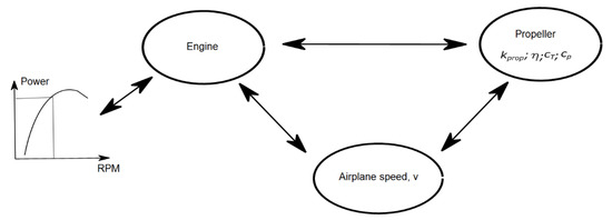
Figure 1.
Model performance triangle, where kprop = propeller stiffness; η = propeller effectivity; cT = thrust coefficient; and v = airplane speed, m/s.
Hypothesis: an increase in the model speed can be achieved by flapping-propeller behavior.
Investigation novelty: the connection between non-steady fluid dynamics behavior and structural stiffness remains complex and ambiguous.
This paper deals with the propellers of class F2 aircraft and their dynamic characteristics. The purpose of the paper is to investigate the influence of the propeller’s construction stiffness on its modal eigenvalues and the effect of the modal eigenvalues on the air model horizontal speed. While the propeller forms were the same for all cases, they differed in matrix stiffness, as the amount of plasticizer in epoxy resin changed. Later, propellers with varying degrees of stiffness were tested with the same air model and engine. In the first part of this article, the physical experiments that were performed are described (Figure 2): (1) an F2 aircraft test with three types of propellers; (2) experiments on the dynamic parameters of the propellers considered. The second part deals with theoretical research.
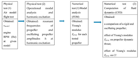
Figure 2.
Main steps in the oscillating propeller dynamics investigation.
2. Materials and Methods
2.1. Experimental Approach
The experimental studies consist of two stages: Physical test 1 and Physical test 2. The aim of Physical test 1 is to analyze the in-flight parameters of a class F2d air model and to determine the influence of different propellers on flight speed (the geometry of the studied propellers is the same; the propellers are of different material stiffness). The following parameters were measured during Physical test 1: propeller RPM and flight speed. Physical test 2 consists of two parts: operational modal analysis and harmonic excitation. The aim of the study is to analyze and determine the dynamic parameters of the investigated propellers (parameters of resonant frequencies and damping coefficients are determined).
The results of Physical test 2, operational modal analysis, are also used to determine the properties of the propeller materials (Section 2.2.1, Numerical Experiment (1)). The purpose of Physical test 2’s harmonic excitation study is to analyze and determine the response of the investigated propellers to harmonic excitation; the excitation frequencies used are the resonant frequencies of the respective propellers, and the frequencies during engine flight with the respective propeller. During Physical test 2, the amplitudes of the significant points of the propeller before the different harmonic excitations are determined. Physical test 2’s harmonic excitation results are used in the modeling (Section 2.2.1, Numerical Experiment (2)).
2.1.1. Physical Test (1)
The physical test was performed with a F2D combat model, which is regulated according to FAI rules. This type of model is controlled by steel lines.
The equipment of this model type was tested with a “Fora” engine, as illustrated in Figure 3. During the physical test, the same model, engine, and fuel were used, as was the same shape of propeller, but with three different propeller stiffness variants. The first is referred to as “C1 original” (prop. 1), which is a propeller mass produced by various manufacturers and with typical propeller stiffness of its type. This propeller was tested with two other propellers, which are referred to as prop. 2 and prop. 3. The variation in the amount of stiffness was obtained by use of a different amount of plasticizer in the epoxy resin during the propellers’ fabrication process.
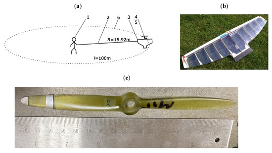
Figure 3.
Basic physical test scheme. (a) 1—test pilot; 2—control line; 3—model; 4—engine; 5—propeller; and 6—model flight path. (b) A detailed view of the F2D-class combat model. (c) C1 propeller type (diameter D = 160 mm; pitch ≈ 95).
During physical testing, the aim was to investigate the influence of propeller stiffness on model speed, as a higher model speed indicates a higher suitability to convert engine power to model speed. The engine (model, Engine FORA 2.5CC F2D two stroke; bore 14 stroke, 15 mm; cooling air; weight, 127 g) in each test was set to maximum power. The engine RPM of each propeller was tested using an R7050 Compact Photo Tachometer and Counter, which has a maximum measurement of RPM from 2 to 99,999 and an accuracy of +/−0.05. The model speed was tested by counting the average time required to fly 10 circles with each propeller, with one circle being equal to 100 m, 10 circles being equal to 100 m × 10 = 1000 m, and v being equal to 1000 m/tflight time.
In Table 1, the averaged values of the physical test are given. In total, three propellers were each tested ten times. The two measured scenarios are as follows: (a) engine RPM and model static vmodel = 0 m/s, and (b) engine RPM and model speed vmodel in horizontal flight. The results of Physical test 1 show that propeller stiffness variations affect the engine rotation speed and model flight speed. This confirms the initial model performance triangle (see Figure 1) in which a change in mechanical property (in this case, propeller stiffness) changes the balance of the flight speed of the whole propeller–engine–model system. A summary of the measured results is given in Table 1.

Table 1.
Summary of the physical test results (the average values of each propellor tested 10 times); 3 propellers × 10 measurements = 30 samples.
The physical test showed that prop. 2 had a higher speed in horizontal flight, while in revolutions (tide loops and other), the drop of the engine RPM ratio between horizontal flight/revolving flight was significantly lower. Since the investigation of revolving flight dynamics is rather complex, in this paper we focus only on the propeller stiffness effect on the models’ horizontal speed. The measured engine RPM and model speed are used for the numerical investigation.
2.1.2. Physical Test (2)
Modal analysis. The purpose of this physical experiment was to predict propeller dynamic instability, which affects propeller aerodynamic parameters. Therefore, operational modal analysis (OMA) of the three different stiffness variants tested in model flight conditions was performed (Table 1).
The experimental test equipment is illustrated in Figure 4. It consists of 3660-D measurement result processing equipment (BRÜEL & KJÆR, Nærum, Denmark) with a PC (Figure 4, items 1.1 and 1.2); parts of this measurement system and the processing of measurement data; noncontact displacement transducers; “Lion precision” (Lion precision, Oakdale, USA) U3B and U20B (items 2.1 and 2.2 in Figure 4) with an amplifier ECA101 (specifications: analog outputs; 0–10 VDC; 0 Ω; 15 mA max; nonlinearity: 0.5%; resolution: 30 nm); and a power supply (item 2.3 in Figure 4) that measures the response of the propeller to external excitation. A 4812 General Purpose Head and a 4805 Permanent Magnet with a 2707 power amplifier (BRÜEL & KJÆR, Nærum, Denmark) were used for the external excitation of the test object (positions 3.1 and 3.2 in Figure 4). Shaker specifications: dynamic rated force–sine peak: 445 N; displacement, peak to peak (max): 12.7 mm.
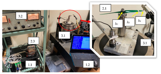
Figure 4.
Equipment required for modal analysis of propellers.
For measurement, the distances of the measuring points h0, h3, and h4 (Figure 4) were set at 0.00, 0.75, and 1.0 R (where R is the radius of propeller) from the propeller part attached to the stand (i.e., from the center of the propeller). Measurements were performed using sweep excitation from 300 to 1600 Hz, with the frequency sweep rate at 500 Hz/s.
The results of the study illustrated in Figure 5 provided the values of modal parameters and mode forms of the first two modes of the three propellers tested. In the graphs of Figure 5, the notations next to the numbers “m” and “u” correspond to the multipliers 10−3 and 10−6, respectively. Each propeller was tested six times: 3 propellors × 6 cases = 18 measurements. The values are given in Table 2.
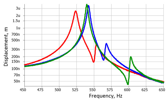
Figure 5.
Graph of edge point h4 (Figure 4) displacement spectral density of the investigated propellers using sweep excitation: red curve—“prop. 3”; blue curve—“prop. 2”; and green curve—“prop. 1”.
Table 2.
Propeller center point h0 and propeller edge point h4 amplitudes during the harmonic excitation test.
Analysis of the results shows that the first two resonant frequencies of prop. 3 were 524 and 556 Hz, with the damping coefficient at 0.51; the first two resonant frequencies and the damping coefficient of prop. 2 were 542 and 568 Hz and 0.33, respectively; and the first two resonant frequencies and the damping coefficient of prop. 1 were 540 and 600 Hz and 0.31, respectively. The analysis of the amplitudes of the propeller points at the first resonant form reveals that the maximum amplitudes of the displacement of the propeller points were found for prop. 3, with the lowest damping coefficient.
Harmonic excitation. Vertical harmonic excitation was applied to the structure by applying harmonic load F0 sin (ωt). After determining the modal parameters of the propellers, a harmonic excitation test was performed (the same equipment was used as in modal analysis (Figure 4) to determine the amplitudes at significant points of the propeller at first resonant frequency and at frequencies generated during operation in flight conditions (i.e., the frequencies resulting from the airplane engine’s revolutions).
Table 2 presents the propeller center point h0 and propeller edge point h4 amplitudes during the harmonic excitation test.
Analysis of the obtained results shown in Table 2 indicates that the input amplitude parameter has a significant effect on the propeller blade-tip-oscillating amplitudes: the blade tip amplitude of prop. 3 at point h4 (Figure 4) exceeded 102 µm, while the other two propellers’ amplitudes exceeded only 19.4 and 37.5 µm or 19.4 and 36.7 percent. The amplitude gradually decreased when approaching the propeller’s center. The discussion of the surface amplitudes of the individual propellers is provided in the section on the numerical experiment (2).
2.2. Numerical Approach
Physical test 1 showed a significant variation in engine RPM and model speed with respect to the variation in propeller stiffness. In Numerical experiment (1), using the “Ansys” finite element method, the longitudinal propeller modulus of elasticity for each tested propeller was calculated, which shows the effect of propeller stiffness variation on model speed.
In Numerical experiment (2), using the finite volume method “ANSYS CFX”, the contribution of propeller rotation, the flapping and flow separation, and the reattachment to the propeller thrust in the measured propellers’ operating conditions were determined.
2.2.1. Numerical Experiment (1)
Physical test 1 showed that propeller stiffness has a relatively significant effect on airplane speed performance.
By using reverse engineering methods in Physical test 2, mode 1 and frequency were calculated using a general FEM equation:
where [M] indicates structural mass matrix, is the acceleration vector, [C] is the structural damping matrix, is the velocity vector, [K] represents the structural stiffness matrix, and {F} is the displacement vector and is the applied load vector for the case of modal analysis {F} = 0.
In this case, we can assume that, according to the stiffness matrix, by changing the amount of plasticizer in the epoxy resin, we only change [K], e.g., [K] ≡ Young’s modulus in Equation (1). Moreover, [M] can be neglected since the propeller shape is the same in all cases. This means that it is possible to calculate the stiffness of the propellers tested from the measured mode eigenvalues.
One of the possible solutions for Equation (1) by using the “Ansys” finite element program is to use a reverse engineering approach—to calculate the actual propeller material matrix Young’s modulus from the modal frequencies measured during Physical test 2.
Generally, the mechanical behavior of composite structures for orthotropic elasticity materials is defined by the properties of nine parameters, such as Young’s modulus, Poisson ratio, and Shear modulus (Ex, Ey, Ez, υxy, υyz, υxz, Gxy, Gyz, and Gxz), for unidirectional layer composites (which were used in this case), where the x-axis runs along the propeller blade and Ey = Ez; υxy = υxz; Gxy = Gxz; and Gyz = Ey/(2(1 + υyz)). This means that we can simplify the modal analysis and investigate its effects on the mode frequency and the matrix Young’s modulus (Figure 6 and Figure 7).
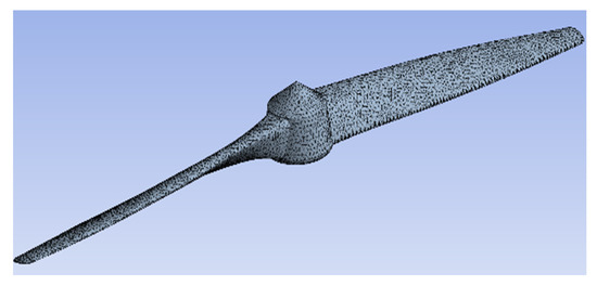
Figure 6.
Propeller mesh for the modal analysis: nodes, 85,400; elements, 53,500.
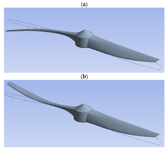
Figure 7.
Propeller modal deformations at Eprop. = 26.8 × 10⁹ Pa: (a) mode 1 frequency at 543.6 Hz; (b) mode 2 frequency at 548.4 Hz.
Figure 8 demonstrates that the original C1 propeller (prop. 1) had a high mode value and a higher Young’s modulus, while those of the other two were ≈3.28 and 9.82 percent weaker, respectively.
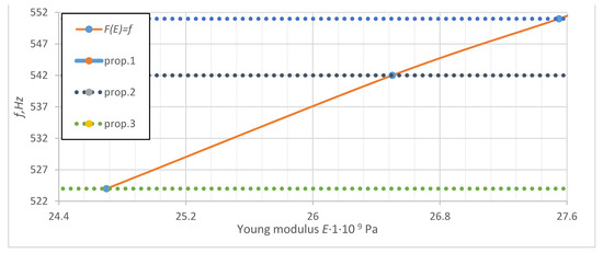
Figure 8.
Mode first frequency f (Hz) eigenvalue and Young’s modulus of the propellers.
2.2.2. Numerical Experiment (2)
A tow domain model consisting of a static rectangle that had long distances from the inlet and outlet was chosen for the investigation based on the minimization of negative effects of the boundary conditions and increased numerical model stability.
The rotation model (Figure 9) had a single blade surface or half of the tested propellers due to propeller symmetricity. The center part of the propeller, which had a very low aerodynamic effect and low flapping amplitude, was not taken into account. Flapping-propeller amplitudes (hi) were applied for each divided propeller surface (Si) individually, according to the data measured in the laboratory for each individual propeller.
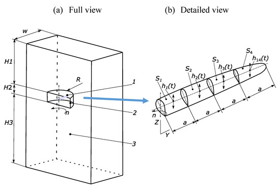
Figure 9.
Numerical model: (a) CAD geometry for the CFD numerical investigation, in which Body 1 is the body of rotation, with speed n (RPM according to the physically measured value); Body 2 is the surface of the wall of the investigated propeller blade (here, Si stands for the flapping area surface); hi is the flapping surface amplitude; a represents the length of the surface at 20 mm; and Body 3 is the static body basic dimensions at H1 = 300 mm, H2 = 70 mm, and H3 = 500 mm. (b) The basic parameters of the flapping blade (Table 2).
The mesh (Figure 10) was generated using a high-quality tetrahedral mesh with 20.4 million nodes and 11.6 elements. Mesh quality was checked using the skewness parameter, the maximum value of which did not exceed 0.82, whereas the average value exceeded 0.2 with a standard deviation of 0.12.
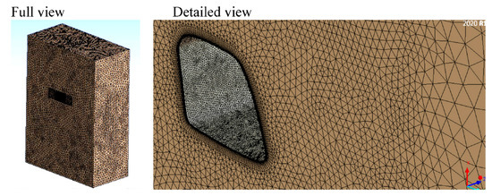
Figure 10.
Mesh of the numerical model. Mesh density in the area next to the propeller surfaces is increased by up to 12 times.
For mesh validation purposes, three different meshes were generated with three different mesh densities around the investigated propeller blade surfaces. In scenario a, the mesh density of the blade surface increased by 34% up to 0.1 mm or 0.00125R of the blade, and the mesh density around the blade increased by up to 0.0075R; in scenario b, the mesh density of the blade surface of 0% increased by up to 0.15 mm or 0.00185R of the blade, and the mesh density around the blade increased by up to 0.005R; but in scenario c, the mesh density of the blade surface decreased by 34% to 0.45 mm or 0.0057R of the blade, and the mesh density around the blade increased by up to 0.0227R. The numerical investigation shows that the results of scenarios a and b (propeller thrust and torque) in both cases were very similar; the difference was less than 1%. In contrast, the result of scenario c was higher at around 10% compared with physical testing. Therefore, mesh generation using scenario b was chosen for further numerical investigations.
Boundary conditions. The same mesh was used in all cases in the numerical model, but different inlet speeds and RPMs were used in Physical test 1; the blade-flapping amplitudes were obtained from Physical test 2.
To capture the blade-to-blade interaction and unsteady flow, rotation periodicity boundary conditions (per1 and per2) for a precise representation of the pass flow effect on the rotation blade were used (Figure 11). Static and rotation body interaction (Dom. inter 1, 2, and 3) was realized using a domain interface frozen rotor model with specified pitch angles.
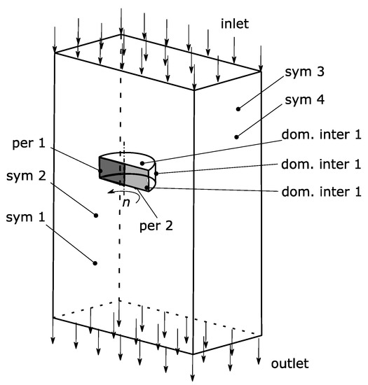
Figure 11.
CFD model boundary conditions, where inlet velocity was applied to a rectangle body according to the physical test results in m/s and with outlet-opening conditions with pressure P = 0.
3. Results
Due to the high complexity of oscillating propeller analysis, at first a propeller static thrust analysis with v = 0 m/s and with an engine speed of 28,600 RPM was performed. At these boundary conditions, the physical model showed 1.3 kg or 12.75 N of thrust. The CFD model showed ≈ 2.1 percent less static thrust for all tested propellers, and Figure 12 illustrates the streamline distribution on the blade’s surfaces. This verification of the numerical CFD model shows high precision and confirms the possibility of using it for the oscillating propeller analysis.
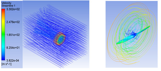
Figure 12.
Streamline distribution in the computer domain.
Investigation of propeller force and drag contribution along the propeller blade given in Figure 13:
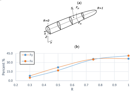
Figure 13.
Thrust force Fy and drag force Fx distribution on the original C1 propeller, according to blade radius R: (a) schematic view; (b) graphic view.
As illustrated in Figure 13, the thrust increased by an increase in R and at the 0.75R of the propeller blade, creating the highest thrust. Later, the thrust started to decrease, while drag force Fx increased in the whole R range. This implies that higher propeller effectiveness is distributed close to the blade tips. Additionally, the highest blade-flapping amplitudes were found here, and the interaction of these two factors is of considerable importance in highly effective propeller design.
Effect of a flapping-propeller blade. A comparison of a transient rigid propeller with a flapping propeller and a transition turbulence Gamma Theta model, which allowed us to simulate laminar, laminar-to-turbulent, and turbulence states in a fluid flow, was made. The Gamma-Re model does not intend to model the physics of the problem but attempts to fit a wide range of experiments and transition methods for its formulation.
For all cases, a shear stress transportation fluid model with two options was used: the full turbulence and the Gamma Theta model (Figure 14). The effect of air separation and laminar flow transition on turbulent flow showed an increase in propeller thrust and required power by ~3.6% due to flow separation occurring near propeller blade surfaces. The combination of the propeller-flapping effect with air flow separation is the key factor for modeling this type of propeller. For precise investigation, it is also necessary to take in to account the behavior of nonconstant propeller deformation from the center to the blade tip and the most effective propeller thrust (lift) and drag (required moment to rotate it at given RPM) generation area. Three propeller operation cases are given in Figure 14 and Figure 15.
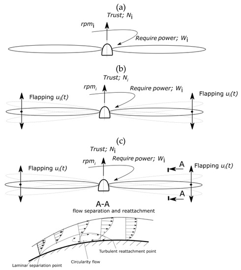
Figure 14.
Comparison of various propeller effects: (a) rigid propeller, (b) flapping propeller, and (c) flapping propeller with flow separation and reattachment.
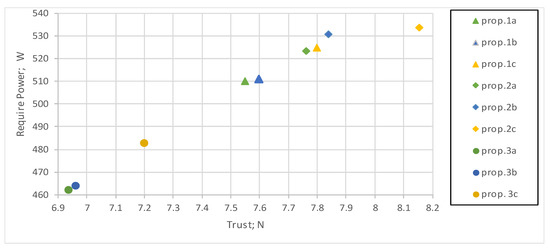
Figure 15.
Propeller thrust and required power sheet generated by CFD analysis, for three propeller stiffnesses and three propeller models effects (see Figure 14). Nomenclature example: prop. 1c = original C1 flapping propeller with the flow separation Gamma Theta model with Physical tests 1 and 2 measured as input parameters (Table 1 and Table 2).
Unsteady flow is a complicated analytical model. As a simplified model for harmonically pitching and plunging thin airfoils, Theodorsen delivered an expression for lift by assuming a planar wake and a trailing-edge Kutta condition in incompressible flow.
A general theoretical Cl(t) lift coefficient equation is given [21] as follows:
Here, C(k) is the complex-valued Theodorsen function with a magnitude of 1; it accounts for the attenuation of lift amplitude and the time lag in lift response from the real and imaginary parts. The first term is the steady-state lift; the second term is due to acceleration effects; and the last term evaluates circulatory effects, where c is half the cord length, α is the angle of attack, h is the plunge motion, and xp is the bending distance from the cord center.
The simplified model of unsteady flow for the flat plate is given in Figure 16.
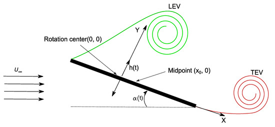
Figure 16.
A simplified model of the unsteady flow oscillating the flat plate. Here, LEV is the leading edge vortex and TEV is the trailing edge vortex.
As illustrated in Figure 17, the analytical model shows that the lift coefficient Cl(t) had higher fluctuations compared with the CFX results. This could be explained by the specific flapping profile, which was taken from the physical test and later used for the CFX analysis.
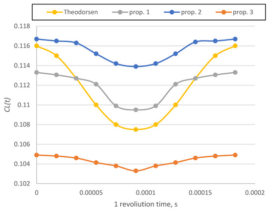
Figure 17.
CL(t) lift coefficient comparison for various propeller cases (revolving in one of these cases) and validation with the theoretical model at point h3 (Figure 4), where ti = time required for one propeller rotation.
Based on the results shown in Figure 18, our main focus is on the propeller airflow parameters at point h3 (Figure 4).
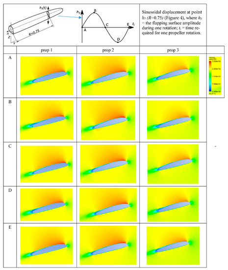
Figure 18.
Flapping-propeller velocity field at point h3 (Figure 4) at set time and amplitude points, where (A–E) are surface h3(t) displacement positions.
As shown in Figure 18, it can be observed that, at positions b and d, there was a TEV vortex formulation on the propeller blade (the blue zone at the top of the blade’s trailing edge), which affected lift force generation by the propeller blade. The authors of [22] stipulate that the thrust and lift coefficient could continuously increase with a heaving amplitude up to a relatively large range (h/c < 1.5), where h represents amplitude and c is blade width. Amplitude is limited by other factors, such as the required propeller stiffness to start the engine by hand, and fatigue of the material. This study shows that a partial decrease in propeller stiffness positively affects propeller aerodynamic characteristics in horizontal flight. Moreover, this study can be extended to a full flight path of an F2D combat model, which consists of combinations of tight loops and straight flight segments.
The flapping propeller velocity field in limit points is shown in Figure 18A–E.
4. Conclusions
Physical tests showed a significant effect of propeller stiffness on the speed of the F2D combat air model for the investigated propellers.
Experimental studies yielded the modal parameters for the three examined propellers. Analysis of the results shows that the frequency of the first resonant form of the investigated propellers varied from 524 to 542 Hz, respectively, and that the frequency of the second resonant form varied from 556 to 600 Hz. The damping coefficients of the first resonant form of the examined propellers varied from 0.31 to 0.51. Analyzing the amplitudes of the significant points of the examined propellers in the first resonant form, it was determined that the maximum amplitudes of the displacement of the propeller points can be found for the three propellers with the lowest damping coefficient.
Analysis of the significant point displacement results of the examined propellers during harmonic excitation showed that, when the excitation frequency was selected according to the aircraft engine speed, the maximum propeller edge displacement amplitudes ranged from 19.1 to 37.5 µm when the propeller attachment point amplitude was 2.2 µm. Evaluation of the results obtained when the harmonic excitation frequency corresponded to the first resonant frequency of the respective propeller revealed that the maximum amplitudes of the propeller edge displacement reached from 81.8 to 107.6 µm.
The change in one triangle participant parameter affected two others. The results of Physical test 1 in Table 1 show that the best speed generated was that of prop. 2 because its spectrum density local maximum (blue color) was very close to the engine RPM (the engine RPM is 34,300 or 571 Hz when local peak is at 575 Hz).
The decrease in the initial propeller “C1” (prop. 1) stiffness by 3.28% increased the propeller’s effectiveness, and flight speed increased by 0.8%. The numerical investigation showed a significant propeller thrust increase when the propeller blade was flapping during its rotation of up to 3.6%, due to the non-steady flow separation and reattachment contribution regime near the trailing leading edge.
Author Contributions
Conceptualization, V.R. and A.K.; methodology, V.R. and A.K.; software, V.R. and A.K.; validation, V.R. and A.K.; formal analysis, V.R. and A.K.; investigation, V.R. and A.K.; resources, V.R. and A.K.; data curation, V.R. and A.K.; visualization, V.R. and A.K.; supervision, V.R. and A.K. All authors have read and agreed to the published version of the manuscript.
Funding
Not applicable.
Institutional Review Board Statement
Not applicable.
Informed Consent Statement
Not applicable.
Conflicts of Interest
The authors declare no conflict of interest.
References
- Anderson, J.M.; Streitlien, K.; Barrett, D.S.; Triantafyllou, M.S. Oscillating foils of high propulsive efficiency. J. Fluid Mech. 1998, 360, 41–72. [Google Scholar] [CrossRef]
- Knoller, R. Die Gesetze Luftwiderstandes. Flug Mot. 1909, 3, 1–7. [Google Scholar]
- Betz, A. Ein Beitrag zur Erklearung des Segelfluges. Z. Flugtech. Mot. 1912, 3, 269–272. [Google Scholar]
- Garrick, I.E. Propulsion of a flapping and oscillating airfoil. NACA Rep. 1937, 567, 419–427. [Google Scholar]
- Benkherouf, T.; Mekadem, M.; Oualli, H.; Hanchi, S.; Keirsbulck, L.; Labraga, L. Efficiency of an auto-propelled flapping airfoil. J. Fluids Struct. 2011, 27, 552–566. [Google Scholar] [CrossRef]
- Chen, Y.M.; Liu, J.K. Nonlinear aeroelastic analysis of an airfoil-store system with a freeplay by precise integration method. J. Fluids Struct. 2014, 46, 149–164. [Google Scholar] [CrossRef]
- Xiao, Q.; Zhu, Q. A review on flow energy harvesters based on flapping foils. J. Fluids Struct. 2014, 46, 174–191. [Google Scholar] [CrossRef]
- Gopalkrishnan, D.S.B.R.; Triantafyllou, M.S.; Triantafyllou, G.S. Active vorticity control in a shear flow using a flapping foil. J. Fluid Mech. 1994, 274, 1–24. [Google Scholar] [CrossRef]
- Streitlien, K.; Triantafyllou, G.S. On thrust estimates for flapping foils. J. Fluids Struct. 1998, 12, 47–55. [Google Scholar] [CrossRef]
- Politis, G.K. Application of a BEM time stepping algorithm in understanding complex unsteady propulsion hydrodynamic phenomena. Ocean Eng. 2011, 38, 699–711. [Google Scholar] [CrossRef]
- Bøckmann, S.; Steen, E. The effect of a fixed foil on ship propulsion and motions. In Proceedings of the Third International Symposium on Marine Propulsors, Launceston, Australia, 13 May 2013; pp. 553–561. [Google Scholar]
- Bøckmann, S.; Steen, E. Model test and simulation of a ship with wavefoils. Appl. Ocean Res. 2016, 57, 8–18. [Google Scholar] [CrossRef]
- Liu, H.; Qu, Z.; Shi, H. Numerical study on hydrodynamic performance of a fully passive flow-driven pitching hydrofoil. Ocean Eng. 2019, 177, 70–84. [Google Scholar] [CrossRef]
- Wu, X.; Zhang, X.; Tian, X.; Li, X.; Lu, W. A review on fluid dynamics of flapping foils. Ocean Eng. 2020, 195, 106712. [Google Scholar] [CrossRef]
- Chen, J.-S.; Chen, J.-Y.; Chou, Y.-F. On the natural frequencies and mode shapes of dragonfly wings. J. Sound Vib. 2008, 313, 643–654. [Google Scholar] [CrossRef]
- Thiria, B.; Godoy-Diana, R. How wing compliance drives the efficiency of self-propelled flapping flyers. Phys. Rev. E 2010, 82, 015303. [Google Scholar] [CrossRef] [PubMed]
- Vanella, M.; Fitzgerald, T.; Preidikman, S.; Balaras, E.; Balachandran, B. Influence of flexibility on the aerodynamic performance of a hovering wing. J. Exp. Biol. 2009, 212, 95–105. [Google Scholar] [CrossRef] [PubMed]
- Spagnolie, S.E.; Moret, L.; Shelley, M.J.; Zhang, J. Surprising behaviors in flapping locomotion with passive pitching. Phys. Fluids 2010, 22, 041903. [Google Scholar] [CrossRef]
- Jankauski, M.; Guo, Z.; Shen, I.Y. The effect of structural deformation on flapping wing energetics. J. Sound Vib. 2018, 429, 176–192. [Google Scholar] [CrossRef]
- Ha, N.S.; Truong, Q.T.; Goo, N.S.; Park, H.C. Relationship between wingbeat frequency and resonant frequency of the wing in insects. Bioinspir. Biomim. 2013, 8, 046008. [Google Scholar] [CrossRef] [PubMed]
- Shyy, W.; Aono, H.; Kang, C.; Liu, H. An Introduction to Flapping Wing Aerodynamics; Cambridge University Press: Cambridge, UK, 2013. [Google Scholar]
- Ashraf, J.C.S.; Young, M.A.; Lai, J. Oscillation frequency and amplitude effects on plunging airfoil propulsion and flow periodicity. AIAA J. 2012, 50, 2308–2324. [Google Scholar] [CrossRef]


Publisher’s Note: MDPI stays neutral with regard to jurisdictional claims in published maps and institutional affiliations. |
© 2021 by the authors. Licensee MDPI, Basel, Switzerland. This article is an open access article distributed under the terms and conditions of the Creative Commons Attribution (CC BY) license (https://creativecommons.org/licenses/by/4.0/).