A Real Time Bolometer Tomographic Reconstruction Algorithm in Nuclear Fusion Reactors

Abstract

In tokamak nuclear fusion reactors, one of the main issues is to know the total emission of radiation, which is mandatory to understand the plasma physics and is very useful to monitor and control the plasma evolution. This radiation can be measured by means of a bolometer system that consists in a certain number of elements sensitive to the integral of the radiation along straight lines crossing the plasma. By placing the sensors in such a way to have families of crossing lines, sophisticated tomographic inversion algorithms allow to reconstruct the radiation tomography in the 2D poloidal cross-section of the plasma. In tokamaks, the number of projection cameras is often quite limited resulting in an inversion mathematic problem very ill conditioned so that, usually, it is solved by means of a grid-based, iterative constrained optimization procedure, whose convergence time is not suitable for the real time requirements. In this paper, to illustrate the method, an assumption not valid in general is made on the correlation among the grid elements, based on the statistical distribution of the radiation emissivity over a set of tomographic reconstructions, performed off-line. Then, a regularization procedure is carried out, which merge highly correlated grid elements providing a squared coefficients matrix with an enough low condition number. This matrix, which is inverted offline once for all, can be multiplied by the actual bolometer measures returning the tomographic reconstruction, with calculations suitable for real time application. The proposed algorithm is applied, in this paper, to a synthetic case study.

1. Introduction

The tokamak is an experimental machine designed to exploit the energy from controlled fusion reaction [1]. In the tokamak configuration, to achieve the temperature and pressure necessary to make the fusion reaction possible, magnetic and electric fields are used to heat and squeeze a hydrogen plasma inside a toroidal camera. No material can withstand the high temperatures needed to sustain the nuclear fusion reaction. One solution is to keep the hot plasma out of contact with the walls of the camera, by keeping it moving in helical paths by means of the magnetic force. To twist the field lines helically, the tokamak features a toroidal field created by a series of coils evenly spaced around the torus-shaped reactor, and it creates a poloidal field by inducing an electric current in the plasma through a central solenoid. The tokamak is the most extensively investigated magnetic confinement concept and, despite multiple technical challenges, it is considered the most promising configuration for the fusion reactor. Many tokamak devices have been built in Europe, UK, USA, China, Russia and Japan. Two important projects are currently under development, ITER and DEMO. ITER aims to demonstrate the scientific and technological feasibility of fusion as a source of energy. DEMO will bring fusion energy research to the threshold of a fusion reactor prototype. In such fusion devices, electromagnetic radiation emission represents a significant quota of the dissipated heating power [2]. Such an energy loss is mainly due to the transport of impurities inside the plasma. Measuring the evolution of the radiation emissivity distribution is crucial, especially in machines with metallic walls, to develop appropriate operational scenarios, investigate magnetohydrodynamic instabilities and maximize the performances [3,4]. In present day experimental devices, such as JET, ASDEX Upgrade and JT-60U [5,6,7], bolometers are used to measure the line integral values of the local radiated emission along viewing chords. Although bolometers measure only the radiated power along the line-of-sight (LOS), by using the measurements from many LOSs it is possible, in principle, to reconstruct the distribution of the local emissivity $\mathsf{\epsilon }\left(r,z\right)$ in the poloidal cross-section of the tokamak by solving the following Fredholm integral equation of the first kind:

$$\iint K_j\left(r, z\right)\mathsf{\epsilon }\left(r,z\right)\mathrm{d}rdz=b_j$$

(1)

where $K_j\left(r, z\right)$ describes the geometry of the diagnostics, $b_j$ is the measure along the j-th LOS, and the coordinates r and z are the horizontal and vertical directions in the poloidal tokamak cross-section.

Several methods have been proposed in literature to invert Equation (1), among which the most widely used in the nuclear fusion area are those belonging to the series expansion methods [8,9]. The series expansion methods consist in discretizing Equation (1) before inverting it. Such discretization, performed by expanding the emissivity in basis functions, leads to a system of linear equations:

$${\displaystyle \sum }_i{K}_{ij}{\epsilon }_i=b_j, i=1,\cdots ,n; j=1,\cdots ,m$$

(2)

where $K_{ij}$ is the geometry matrix, ${\epsilon }_i$ is the local emissivity at the i-th grid point, n is the number of grid points and m is the number of chords. Usually, the discretization is performed on a regular rectangular grid, even if grid elements with different shapes have also been used [6,10,11].

Solving the linear system in (2) is referred to as the tomographic reconstruction problem, i.e., reconstructing the 2D plasma emissivity distribution in the poloidal tokamak cross-section starting from an often limited number of line-integrated, noisy, measures of the plasma radiation.

Even if a number of algorithms have been developed to solve the tomographic problem in (2) for the most important tokamaks, such as JET [9,12], ASDEX Upgrade [13,14,15], JT-60 [16], DIII-D [17] and also for the design of ITER [18], there are intrinsic difficulties common to all of the nuclear fusion experiments:

–

Limited number of LOSs due to the restrictions to access the view of the plasma through the available ports in the vessel;

–

Uneven spatial coverage;

–

Noisy measurements.

These constraints lead to a greatly undetermined, very ill-posed, tomographic inversion problem according to Hadamart [11], whose solution can be addressed with regularization techniques that introduce additional information on the subject problem. In the iterative methods, such as ART and SIRT [8,19,20], the additional information consists in providing a starting solution which both methods iteratively modify by minimizing the difference between the present measures and those calculated in the previous iteration. The procedure is iterated until a stopping criterion is fulfilled. Of course, the solution is heavily affected by the starting point and the convergence time can be prohibiting for real-time applications.

In a nuclear fusion experiment, at each discharge, a large amount of bolometer data is acquired; hence, the tomographic reconstruction is a very heavy task. Nevertheless, being able to reconstruct the distribution of the local emissivity with sufficient accuracy and speed could be crucial to enable its use in the real time control system. The majority of the proposals in literature in the nuclear fusion environment belong to the so-called constraints optimization methods.

In the Phillips–Tikhonov regularization, a functional $\mathsf{\Lambda }\left(ϵ\right)$ is minimized by the method of Lagrange multipliers. The functional usually includes the measures residuum and a regularization function that considers both the anisotropic smoothness of magnetic flux surfaces and some boundary constraints [15,18]. The algorithm searches for a solution where the emissivity distribution is constant on flux surfaces and gently varies in the radial direction. As an example, for ASDEX Upgrade, in [15] the following functional is assumed:

$$\mathsf{\Lambda }\left(ϵ\right)={\left(\mathit{K}\mathit{\epsilon }-\widehat{\mathit{b}}\right)}^T{\mathbf{\Sigma }}^{-1}\left(\mathit{K}\mathit{\epsilon }-\widehat{\mathit{b}}\right)+\lambda O\left(\mathit{\epsilon }\right)$$

(3)

where $\widehat{\mathit{b}}$ is the vector of the actual measures subject to experimental errors. Hence, the first term is the residuum weighted by the expected covariance matrix $\Sigma$. $O\left(\mathit{\epsilon }\right)$ is the regularization functional that is set as a quadratic form $O\left(\mathit{\epsilon }\right)={\mathit{\epsilon }}^T\mathit{H}\mathit{\epsilon }$, with a symmetric and positive semi-definite operator $\mathit{H}\in {\mathit{R}}^{\mathit{n},\mathit{n}}$ which can be a function of $\mathit{\epsilon }$.

The information entropy of the emissivity distribution $-{\displaystyle \sum }_i{\epsilon }_i\ln {\epsilon }_i$ has been assumed as regularization functional in the Maximum Entropy method [21] for KSTAR and TCV data, whereas in the minimum Fisher Information method [22,23], the non-linear Fisher Information I_F:

$$I_F=\iint \frac{\epsilon \prime \left(r,z\right)}{\epsilon \left(r,z\right)}drdz$$

(4)

is minimized for TCV. By dividing the first derivative of emissivity distribution by emissivity $\epsilon$ itself assures that smoothness is stronger in regions of lower $\epsilon$ and vice versa.

In [24,25] the Maximum Likelihood method was implemented for the bolometer tomography at JET, where the likelihood probability density function was assumed to follow the error statistics of the experimental data. In this case as well, the a priori information states the smoothness along the magnetic surfaces, given by the plasma equilibrium.

In JT-60 [16], the regularization functional is given by:

$$\mathrm{O}\left(\epsilon \right)=\int {\left({\nabla }^2\epsilon \left(r,z\right)\right)}^{2}drdz$$

(5)

The constrained optimization problem consists in simultaneously minimizing the error between the measured signal and the fitted profile, and the smoothing function $\mathrm{O}\left(\epsilon \right)$.

In the spherical tokamak Globus-M, the anisotropic diffusion regularization functional is represented using the perpendicular and parallel components of the poloidal magnetic flux:

$$\mathrm{O}\left[\epsilon \left(r,z\right)\right]=\iint {\left[\nabla \left(\mathit{n}{D}_{\perp }\mathit{n}\nabla \epsilon +\mathit{t}{D}_{\parallel }\mathit{t}\nabla \epsilon \right)\right]}^{2}drdz$$

(6)

where $D_{\perp }$ and $D_{\parallel }$ are the coefficients which correspond to the perpendicular and parallel magnetic flux directions, respectively.

All the proposed approaches assume that the magnetic plasma equilibrium, hence the magnetic flux surfaces, be available during the discharge evolution. That, together with the time-consuming optimization procedure, prevents the monitoring of the plasma radiation across an entire discharge.

The present contribution aims to overcome these limits by using the a priori information on the statistical distribution of the radiation emissivity over a large amount of tomographic reconstruction performed off-line. Moreover, the domain discretization is done by relying on the line of sights of the bolometer. As the LOSs can be not uniformly distributed, the resulting grid can be uneven too, and the more interesting regions, such as the plasma core and divertor region, are more densely discretized. The a priori statistical information is used to reduce the number n of grid elements in order to obtain a square geometry matrix ${\mathit{K}}_{\mathit{m},\mathit{n}}$ with $n=m$. To this purpose, a regularization procedure is performed, which merge highly correlated grid elements providing a resulting matrix with an enough low condition number. In such a way, solution of Equation (2) can be obtained in real time allowing to monitor the discharge evolution. The analysis of algorithm performance has been done using phantom radiation profiles and virtual channels, similar to the design of tokamak’s lines of sight, showing encouraging results.

The manuscript is organized as follows: Section 2 reports the fundamentals of the proposed method, which consists of two separate procedures: the offline procedure, detailed in Section 3, and the online tomographic reconstruction, reported in Section 4. Section 3 is organized in subsections reporting the different steps of the offline procedure: the construction of the mesh, which makes use of the set of the bolometer LOS, is reported in Section 3.1; Section 3.2 describes the procedure to evaluate the inverse of the square geometry matrix of the bolometer tomography; an algorithm to smooth the obtained tomographic reconstruction is described in Section 3.3; Section 3.4 refers to the offset removal. The proposed method has been described referring to a synthetic case study whose results are presented in Section 4. In Section 5, we discuss the limits and the future perspectives of the proposal.

2. Method Description

In this paper, an a priori regularization method is presented, which allows to evaluate offline the inverse of the square geometry matrix of the bolometer tomography, allowing to solve online the inversion problem by simply multiplying this matrix by the actual measures vector.

The first stage consists of defining a mesh guided by the set of viewing chords, or rays, of the bolometer, in such a way that each cell of the mesh is crossed by only two rays. The number of obtained cells and, consequently, the number of unknowns of the tomography, is much greater than the number of rays, which correspond to the number of equations in (2). As a consequence, the equation system to be solved is underdetermined, which is an inseparable characteristic of tomography. As already highlighted, the undetermined nature of the problem is usually compensated by minimizing a functional, which represents the a priori knowledge of the system under study. The drawback of these approaches is that the functional depends on the measures, and therefore it cannot be optimized offline. This could represent a serious limit in monitoring the nuclear fusion reactors, where a timely intervention is necessary to react to phenomena with very rapid evolution, such as in case of disruption. For this reason, the approach proposed in this paper eliminates the indeterminacy of the problem by leveraging on the behavior of the system, evaluated from a statistical point of view. To this end, a proper dataset of solutions has to be collected. Such dataset should be obtained by applying classical tomographic approaches, which can be applied only offline. The accuracy of the reference dataset is essential for the good performance of the method.

For each cell and for each example in the dataset, the average radiation is considered and the correlation between all the pairs of cells is evaluated. Then, a ranking is defined for the pairs of cells in function of the correlation coefficient, and the most related pairs provide as many regression equations to be added to the tomographic equations in (2).

As a very preliminary assumption, linear correlation between pairs of cells is considered:

$${\epsilon }_j={\alpha }_{ij} {\epsilon }_i+s_{ij}\left( {\epsilon }_i\right)\hspace{1em}\hspace{1em}i,j=1,\cdots ,n$$

(7)

where ${\epsilon }_j$ and ${\epsilon }_i$ are the emissivity of the two related cells, ${\alpha }_{ij}$ is the angular coefficient of the regression line, $s_{ij}\left( {\epsilon }_i\right)$ is the residual error, and $n$ is the number of cells.

Note that, in present experimental fusion machines, the investigated operational space evolves continuously with the aim of defining the most efficient parameter configuration for the next step reactors. Several combinations of plasma parameters and different regimes at which the machine operates may lead to different assumptions for correlation among the radiates power of cells, and the hypothesis of linearity could not be reliable. However, in present machines, the investigation of the operational space takes place through preprogramed experiments, for which the correlation between cells can be assessed by a statistical analysis. Thus, the most fitting hypothesis can be set in advance for each experiment. On the contrary, next step fusion reactors will operate in a predefined operational condition, which cannot change significantly. Therefore, the assumptions on the cell correlations can be tailored on the actual operating condition. In future work, nonlinear relations will be investigated.

The number of additional equations (7), namely the number of pairs, has to guarantee that the equation system is determined; therefore, such number must be equal to the difference between the number n of cells and the number m of rays. Special care is paid to choose these additional equations keeping low the conditioning number of the resulting $n\times n$ matrix. Each additional equation is then used to eliminate, by substitution, one of the two unknown radiations from the overall equation system, resulting in a $m\times m$ matrix. In this way, the order of the coefficients matrix is equal to the number of rays, rather than the number of cells. Hence, each unknown in the final system is the radiation of a cell, which represents a set of cells. The coefficient of this unknown in the equation related to a generic ray is equal to the sum of the intersections between the considered ray and the set of cells represented by it.

As a full-rank squared coefficient matrix is obtained, it can be inverted, so that, to solve the tomography, one has to simply multiply the measures of the bolometer by a matrix.

Once the radiations of the representative cells are determined, the radiation of all the other cells can be determined by means of the additional equations. The last step consists of smoothing the solution.

Note that the number of rays determines how fine the mesh is. As expected, the more information is provided to the algorithm, the better is the results. The main reason of this is that in a small cell the average radiation tends to be close to the values in its pixels. This firstly has a positive effect on the correlation among the cells because we can assess which cells are highly related and which one do not. Secondly, in the online procedure the intersection between the ray and the cell could correspond to a peripheral part of the cell; therefore, if the radiation profile within the cell is not constant, the radiation of the cell is “seen” different from the average value. This introduces an error in the constant terms of the tomographic linear equation system. Nonetheless, as highlighted in the previous section, the bolometer setup in real machines has several constrains, then to make significant the study, we assumed a bolometer which features are like those of existing experimental setups.

In the following Section 3, the steps of the off-line procedure are detailed, which have been implemented to reduce the online calculations to mere products of matrices.

3. Offline Procedure

A phantom case study is used in this paper in order to illustrate the method. A set of tomographic images of a tokamak retrieved from the literature (see Figure 5 in [25]) have been assumed as reference dataset. The basis assumption is that these reconstructions have a high level of accuracy; therefore, we assume that the measurements performed on those images are equivalent to the measurements acquired on the real machine. The dataset is used in order to describe the method, and then its relevance in statistical terms is not taken into account here. In a similar way, both the position of the cameras and the number of rays is not corresponding to a really implemented measurement system, but the layout of the bolometer aims to represent a possible configuration. In Figure 1, the set of rays is represented. The bolometer consists of three cameras, recognizable by the color of the corresponding rays (red, green and yellow). The position of the cameras and both number and direction of rays for each camera have been set in order to obtain a fine mesh in the areas where the spatial gradient of the radiation is expected to be higher. In total, the rays amount to 103.

In Figure 2, the schema of the offline procedure is shown, which will be described step by step in the following sub-sections.

3.1. Tessellation of the Area and Meshing

The set of rays is used to build a mesh that optimally exploits the information coming from the rays themselves. Firstly, a tessellation is made on the area, in such a way that the sides of each tile are treats of rays; hence, the tiles are not crossed by any ray. In the case study, the tiles can be delimited from a minimum of three up to six rays, with a corresponding number of sides. The closure of the external tiles is guaranteed by the envelope line of the points of intersection among the rays and the boundaries of the image (Figure 3). Each tile is associated to an identifier point, corresponding to the barycenter of the tile vertices. In Figure 3, these points are indicated by dots. In total, 2510 tiles were obtained.

Starting from the tessellation in Figure 3, the meshing is defined in such a way that the rays cross the cells rather than to be tangent to them.

The segments, which join the barycentres of the tiles having one side in common, form the mesh (see in Figure 4 a portion of the obtained mesh). In the considered example, 4915 segments, representing the sides of the cells in the mesh, have been obtained. The resulting mesh has 2406 cells.

As it can be noted, apart from the number of sides of the involved tiles, and provided that no more than two rays intersect in the same point, all the cells of the mesh have four sides, and consequently, each cell is crossed by only two rays (see Figure 4).

In Figure 5 the obtained mesh is shown (green lines). As it can be noted, the mesh is finer in the plasma region, whereas it is coarser in the peripheral region of the image, which is outside the vacuum vessel. As the solution of the equation system provides a constant solution in the cell, it is important that the size of the cells is small in the regions where strong gradients are expected. This is the reason the three beams of rays are concentrated on the bottom region, which corresponds to the position of the divertor [5] characterized by a high heat flux (Figure 1). At the same time, a fine mesh is required at the top of the plasma cross-section, even if the absolute value is not particularly high, but the spatial gradient is. Finally, the regions near the cameras have fine mesh, even if the radiation could be negligible (e.g., right bottom of the mesh). This is not an issue, because the cells in these regions are strongly related, and then they will be the first ones to be selected for the pairings.

3.2. Cells Pairing and Matrix Inversion

As introduced in Section 2, the cells are paired on a statistical basis, according to the set of reference images. Each cell of the mesh in an image of the dataset is associated to its average radiation, evaluated referring to the gray scale of the pixels in the cell. Hence, a distribution of average radiation is associated to each cell in the entire dataset. Note that, when the average radiation of a cell is equal to the known background value, this value is directly substituted in the overall equation system, whose order correspondingly reduces. This action yields to a strong reduction of the number of variables, as in general the rays cover a region of the vessel which is larger than the area where the plasma is confined. In the present case, this operation allowed to reduce the number of variables from 2406 to 1040. Because of this reduction, some of the rays are no longer useful, as they intersect only cells with background radiation. In the case study, this led to reduce the number of rays to 93. This is a sign that the rays are not properly oriented, a proper choice of the rays should avoid this drawback, for example by concentrating the rays in more interesting areas.

A further reduction of the order of the system is performed by exploiting the relation between pairs of cells, which allows to solve one of the two unknown radiations as a function of the other. The relation among cells depends on how fine the mesh is, and on the different states of the plasma. In fact, we expect that the mesh is so fine that the radiation within each cell is almost constant, and it is probable that, if the database is large, the relationship among the cells radiation will be nonlinear. The characterization of the plasma and the consequent optimization of the rays set is beyond the scope of the present work. To illustrate the procedure, in the following Section 4, an example is shown where statistics are evaluated on a set of frames which makes reliable the assumption of a linear correlation. Further investigation will be performed in future works to set proper relations between pairs of cells depending on their location and plasma operations.

All the pairs of cells are ranked according to the correlation between their distributions, and the ones with highest score are the candidates for the substitution. In case each cell in the candidate pair assumes the same radiation in the entire dataset, the scatter diagram reduces to only one point, and the correlation coefficient no longer can be defined. Nevertheless, this kind of pair has priority in the selection, because one of the two unknown radiations can be determined as a function of the other without uncertainty.

An important issue concerning the condition number of the coefficient matrix must be considered when a candidate pair is selected for the substitution. In fact, in case the final matrix of coefficients is ill-conditioned, the solution of the system is instable. In the unknown substitution procedure, two independent objectives have to be considered, i.e., the condition number, which has to be as low as possible, and the correlation between pairs of cells, which has to be as high as possible. As a matter of fact, by monitoring only the condition number, pairs with weak correlation could be chosen, and furthermore we are not guaranteed that the final matrix is full rank. On the other hand, if only the correlation is considered, the condition number of the final matrix could be extremely high.

In this work, the following iterative procedure is adopted, which represents a compromise between the two objectives. The correlation is evaluated for all the possible pairs of cells, and a corresponding ranking is defined. At each iteration, the condition number of the current matrix is used as a reference, and the ranking is scrolled from the highest correlation until a pair is found that does not get the conditioning number worse than a prefixed threshold. One of the unknowns of the selected pair is then substituted as a function of the other, which becomes the representative unknown of the pair. The procedure is iterated until the matrix becomes squared.

In the present case study, the resulting 93 × 93 coefficients matrix has a condition number equal to 561, which guarantees a sufficiently low sensitivity of the solution to the noise. In Figure 6, the result of the cells pairing procedure is shown, where each color identifies a group of cells associated to the same representative.

3.3. Smoothing

The obtained square coefficients matrix can be inverted offline, so that the online solution of the tomography problem reduces to a matrix product. However, the obtained tomographic solution, even if consistent with the bolometer measures, assigns a unique value to each cell, yielding a discretized profile. Hence, a smoothing procedure should be applied, which would still be consistent with the measures. Several approaches are present in literature to smooth a discretized image [26]. In this paper, a piecewise linear interpolation procedure has been used, which produces an interpolation matrix to be multiplied by the average radiations of the cells.

3.4. Bolometer Measures Offset

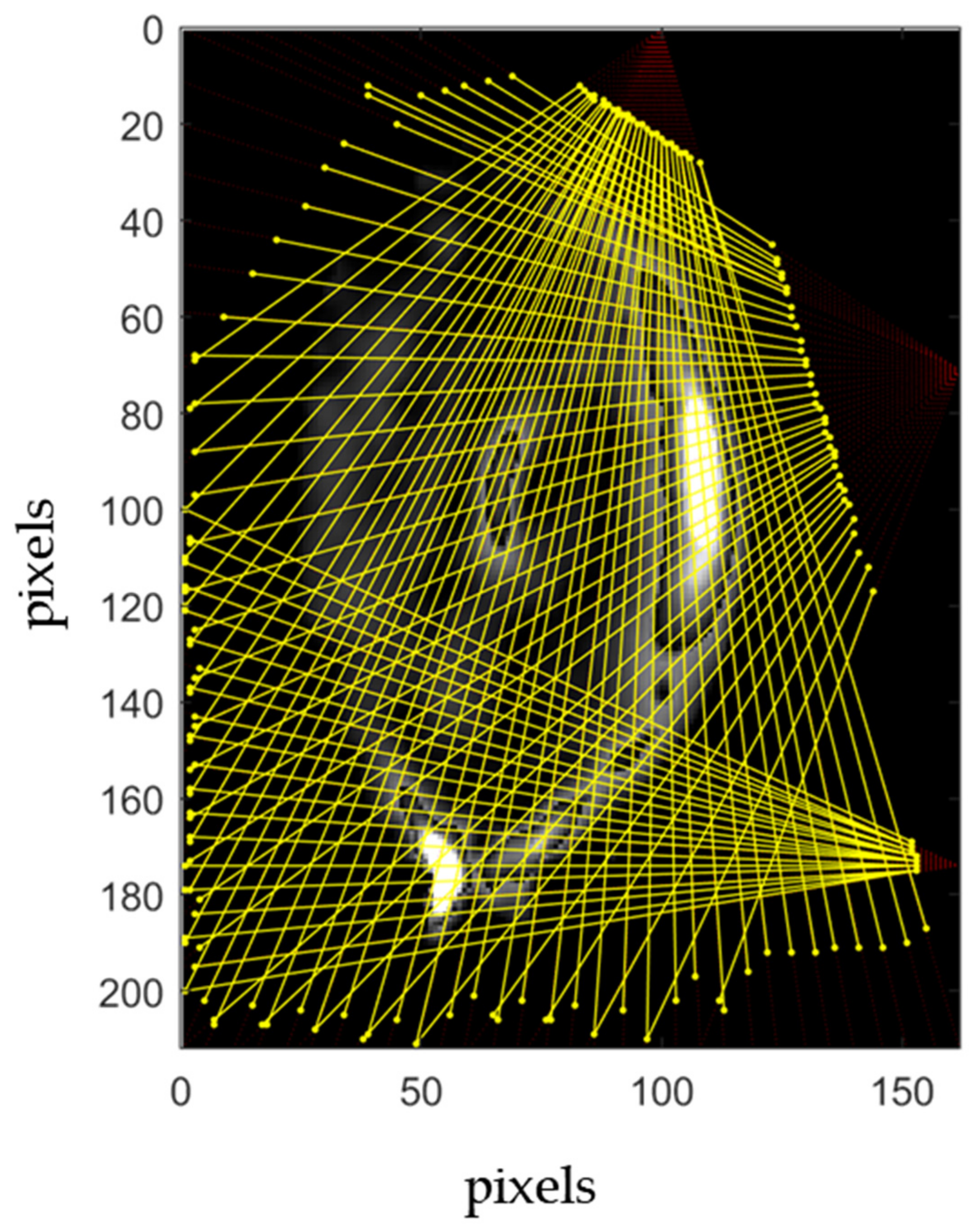
As the Equation (2) can provide information only on the area covered by the mesh, an offset has to be applied to the bolometer measures, corresponding to the traits of rays outside the mesh. In Figure 7, the yellow lines represent the traits of the rays within the area covered by the mesh in the case study. For each ray, the offset can be evaluated a priori by multiplying the length of the trait of ray outside the mesh by the background radiation value, which is assumed constant in the dataset.

4. Online Tomography Reconstruction

The online procedure for the tomographic reconstruction is depicted in Figure 8, which consists of simple algebraic operations. The blocks framed in red in Figure 8 represent the inputs to the online procedure coming from the offline procedure. This last has been carried out, once and for all, with reference to the bolometric system installed in the considered tokamak. In black, in the same Figure 8, the different steps of the online procedure are reported:

• The off-set is removed from the array of measures coming from the bolometer;
• The resulting array of measures is multiplied by the inverted coefficients matrix yielding the radiation of the representative cells;
• The radiations of the other non-representative cells are calculated by means of their relations with the representative ones. Note that this step could be completely parallelizable because each dependent cell is explicitly defined as a function of only one representative cell;
• The final step consists of multiplying the interpolation matrix by the radiation of the cells, obtaining the final tomographic reconstruction.

A test of the running time of the online procedure has been performed on a laptop equipped with an Intel(R) Core (TM) [email protected] CPU, 16 GB of RAM, and Matlab 2020b running in serial mode under Windows 10 (but a similar performance is expected with other setups) and an average computation time equal to about $0.8 \mathrm{ms}$ has been obtained. The computation time can be significantly reduced using a dedicated workstation, and it can be estimated by accounting the number of multiplications performed in the online procedure. Let be m the number of rays, $n$ the number of cells, and $HxL$ the size in pixels of the image, the number of multiplications are $m^2$ in the second step, and $\left(n-m\right)$ in the third step. The fourth step depends on the interpolation algorithm. The one adopted in this work requires at most 30 multiplications per pixel, then $30\left(H\times L\right)$ multiplications in total. In the example described in this paper, the number of multiplications to be accounted are about 1,000,000, then the computation time is in the order of a few microseconds. This makes the reconstruction rate compatible with the sampling rate of the bolometer system, which is of the order of few kHz (e.g., 5 kHz at JET).

In order to validate the proposed procedure, the images of the reference dataset in Figure 5 in [25] are used. The measures of the bolometer have been simulated by integrating the gray levels of the test image along the yellow ray traits in Figure 7. This equals to remove the offsets from the bolometer actual measures.

As said above, the quality of the reconstruction strictly depends on how fine the mesh is, and on the appropriateness of the relationships between the radiations of the pairs of cells. In order to illustrate the procedure, in this example, the correlations have been evaluated on an interval of 1.5 s, to make reliable the hypothesis of linear correlation (see 3.2). Referring to Figure 5 in [25], each sequence corresponds to the frames on the same row.

In Figure 9, the results of the proposed procedure are shown for three frames of the available sequence in the interval [48.1 s–49.5 s] (see Figure 5 in [25]), where the discretized and smoothed tomography reconstructions are compared with the original image. On the top of the original images, the occurrence instant of each frame is indicated, while the average of the relative absolute error on the pixels of each frame is reported as label on the bottom. The relative absolute error for each pixel is calculated as:

$$E\left(x,y\right)=\frac{\left|I\left(x,y\right)-T\left(x,y\right)\right|}{I\left(x,y\right)}$$

(8)

where $I\left(x,y\right)$ is the gray level of the pixel $\left(x,y\right)$ in the original image, while $T\left(x,y\right)$ is the gray level of the same pixel in the smoothed solution. The error on the entire image is defined as the mean squared of $E\left(x,y\right)$:

$$mse=\frac{1}{N}{{\displaystyle \sum }}_{\forall \left(x,y\right)}E{\left(x,y\right)}^2$$

(9)

where $N$ is the number of pixels of the image.

In Figure 10, the reconstructions of other three different frames are reported, which belong to the sequence corresponding to the interval [51.1 s–52.5 s] in Figure 5 in [25].

Due to a more regular trend of the plasma during the first sequence, the accuracy of the reconstruction reported in Figure 9 is better than that in Figure 10, even if the MSE has the same order of magnitude. In fact, the reconstructed images in Figure 10 are affected by the fact that in the considered sequence there is a sudden change of plasma state (see Figure 5 in [25]), and then the hypothesis of linearity is less reliable than in the first sequence. Anyway, the tomographic reconstruction has been able to capture the main feature of the plasma, such as a strong emission in the core at the instants 52.1 s and 52.4 s, the high emission in the divertor and the medium radiation on the left of the core.

5. Discussion and Future Work

As shown in the referenced literature, measuring the evolution of the plasma radiation on the poloidal cross-section of a tokamak device is crucial to monitor the plasma state during an entire discharge. The tomographic reconstruction, providing a 2-D image of the plasma radiation, is very useful to monitor the chain of events during a discharge, distinguishing different phenomena, such as impurity transport and accumulation into the plasma, plasma heating and even disruptions [25]. However, the reconstruction process implemented up to now in the tokamak devices, is time consuming and not compatible with the real time requirements of the monitoring operations.

In our very preliminary proposal, an alternative approach to the tomographic reconstruction is presented, which should overcome this limit, providing a solution by simply performing some matrices products, therefore with very short calculation times. The conclusions are yet to be drawn; however, the preliminary results give us confidence that we can demonstrate the real applicability of the proposed alternative method to real cases. Future work will be then oriented in the construction of a large data base, tailored to a specific tokamak device, with high-definition and non-synthetic images and measurements.

Several strategies can be adopted to improve the accuracy of the reconstructions. Firstly, the hypothesis of linear relations between cells has to be relaxed, and further studies are mandatory to investigate such relations. For example, nonlinear regression of artificial neural network models trained on the available dataset should be applied, providing higher accuracy. Furthermore, important information can be obtained by considering the dynamics of the plasma, by leveraging on possible relationships among consecutive frames. Moreover, the accuracy of the reconstructions could be ideally improved also by optimizing the set of rays to obtain a finer mesh where the profile of the plasma presents a large variation. In fact, as the variables of the tomography equation system are the average radiation in the cells, an error is introduced any time that the radiation changes along the intersection between a ray and a cell. A finer mesh would also contribute to make the hypothesis of linear relation between pairs of cells more reliable. However, as mentioned in the introduction, there are intrinsic difficulties, common to all of the nuclear fusion experiments, which prevent to have mesh size as high as it would serve.