
Some Extremal Graphs with Respect to Sombor Index


1
Department of Mathematics, Sungkyunkwan University, Suwon 16419, Korea
2
Department of Computer and Information Sciences, Northumbria University, Newcastle NE1 8ST, UK
*
Authors to whom correspondence should be addressed.
Mathematics 2021, 9(11), 1202; https://doi.org/10.3390/math9111202
Submission received: 18 April 2021
/
Revised: 19 May 2021
/
Accepted: 20 May 2021
/
Published: 25 May 2021
Abstract
:Let G be a graph with set of vertices and edge set . Very recently, a new degree-based molecular structure descriptor, called Sombor index is denoted by and is defined as , where is the degree of the vertex in G. In this paper we present some lower and upper bounds on the Sombor index of graph G in terms of graph parameters (clique number, chromatic number, number of pendant vertices, etc.) and characterize the extremal graphs.
1. Introduction
Let be a graph with vertex set and edge set , where and . If the vertices and are adjacent, we write . For , let be the degree of the vertex . The maximum degree of a graph G will be denoted by . A vertex of degree 1 is called a pendant vertex (also known as leaf), the edge incident with a pendant vertex is called a pendant edge. For any two nonadjacent vertices and of a graph G, we let be the graph obtained from G by adding the edge . For a subset W of , let be the subgraph of G obtained by deleting the vertices of W and the edges incident with them. Similarly, for a subset of , we denote by the subgraph of G obtained by deleting the edges of . If and , the subgraphs and will be written as and for short, respectively. The chromatic number of a graph G, denoted by , is the minimum number of colors such that vertices of G can be colored with these colors in order that no two adjacent vertices have the same color. A clique of graph G is a subset of such that in , the subgraph of G induced by , any two vertices are adjacent. The clique number of G, denoted by , is the number of vertices in a largest clique of G. For two vertex-disjoint graphs and , we denote by the graph which consists of two components and . As usual, , , and , denote, respectively, the path, the cycle, the star and the complete bipartite graph on n vertices. Other undefined notations and terminology on the graph theory can be found in [1].
A topological descriptor is a numerical descriptor of the topology of a molecule. These topological descriptors are used for predicting the physico-chemical and/or biological properties of molecules in quantitative structure-property relationship (QSPR) and quantitative structure-activity relationship (QSAR) studies [2,3]. In the literature, several degree- and distance-based topological descriptors were proposed and studied by some researchers [4,5,6,7,8,9,10,11,12,13,14,15,16,17]. Very recently, a new degree-based molecular structure descriptor was introduced, the Sombor index is denoted by and is defined as follows [18]:
Many fundamental mathematical properties such as lower and upper bounds can be found in, e.g., [3,10,18,19,20,21,22,23,24,25,26]. This topological index was motivated by the geometric interpretation of the degree radius of an edge , which is the distance from the origin to the ordered pair .
Denote by the set of connected graphs of order n with clique number . The long kite graph (see, Figure 1) is a graph of order n obtained from a clique and a path by adding an edge between a vertex from the clique and an endpoint from the path. In particular, for , . Let . For , we have
and hence
In this paper, we present a lower bound on of graph G in terms of n and clique number , and characterize the extremal graphs.
Theorem 1.
Let . Then with equality holding if and only if .
Corollary 1.
[18] Let G be a connected graph of order n. Then with equality holding if and only if .
Proofof Corollary 1.
Let be the clique number of graph G. Then . Therefore one can easily see that
hence we obtain the required result. □
Let be the set of connected graphs of order n with chromatic number k. Recall that the Turán graph is a complete k-partite graph of order n whose partition sets differ in size by at most 1. When , the only graph in is . So, we now assume that where , i.e., in . We now give an upper bound on of graph G in terms of n and chromatic number k, and characterize the extremal graphs.
Theorem 2.
For any graph , we have
with equality holding if and only if .
Recall that a short kite graph obtained by adding pendant vertices to the unique vertex of clique ; see Figure 2. Let . We have
and hence
Finally we give an upper bound on Sombor index in terms of n, p pendant vertices, and characterize the extremal graphs.
Theorem 3.
Let G be a graph of order n with p pendant vertices. Then
with equality holding if and only if .
2. Preliminaries
From the definition of Sombor index, we have
Lemma 1.
Let G be a graph. Then , where e is any edge in G.
Lemma 2.
[18] Let T be a tree of order n. Then with equality if and only if .
Lemma 3.
[10] Let T be a tree of order with . Then .
In [10], the following two sets are defined:
The following result has been proved in [10].
Lemma 4.
[10] Let T be a tree of order n. Then .
3. Proofs
Proof of Theorem 1.
For , we have and hence the equality holds. For , is a subgraph of G as . Hence by Lemma 1, we obtain
with equality if and only if . For , we have or is a subgraph of G, where is a tree of order n. By Lemmas 1 and 2, we have . Moreover, if and only if .
Otherwise, . Since the clique number of G is , we can assume that a clique of G is . Let H be a connected graph with such that and , where are the trees with , , and . Moreover, . By Lemma 1, we have with equality if and only if . For , we have and . Moreover, for and . Thus, we have
Claim 1.
For , with equality if and only if .
Proof of Claim 1.
Let
For , then the equality holds in Claim 1. For , then
as , the inequality strictly holds in Claim 1. Otherwise, . First we assume that . Thus, we have or . When , we obtain
as and . When , we obtain
as and .
Next we assume that . Since with Lemma 3, we obtain
Claim 1.
is proved. □
Claim 2.
with equality if and only if with .
Proof of Claim 2.
Let
Since and , we have . For , we have the equality holds in Claim 2. Otherwise, . We have . First we assume that . Thus, we have or . If , then we obtain
The equality holds in Claim 2. Otherwise, . We consider two cases:
Case 1.
. In this case
as .
Case 2.
. We obtain
as and .
Next we assume that . Then . If , then and one can easily check that Otherwise, . We consider the following two cases:
Case 3.
. Let be a vertex adjacent to in tree . Then as . First suppose that . Then . One can easily see that
as .
Next suppose that . In this case . Since is a tree of order , by Lemma 3, we obtain
Case 4.
. For , one can easily check that . So now we have . Since and is a tree, , (say), where is a tree of order with . Thus, we have . Let be a vertex in such that , where . We now prove that
First we assume that . Then by Lemma 3, . We obtain
the result strictly holds in (4).
Next we assume that . For , we have , for , and hence we obtain
The equality holds in (4). Otherwise, . In this case and for . If , then one can easily check that the result holds in (4). Otherwise, . We obtain
or
One can easily check that
Again the result holds in (3).
Using the result in (3), we obtain
If , then from (5), we obtain
as . Otherwise, . In this case . From (5), we obtain
as . Claim 2 is proved. □
Using Claim 1 and Claim 2, we obtain
with equality if and only if and with , i.e., .
Since , we have and . Using the above result in (3), we obtain
This completes the proof of the theorem. □
Let be positive integers with . Denote by a complete k-partite graph of order n whose partition sets are of size , respectively. We will determine the extremal graph in with respect to Sombor index of graphs G. For this we first prove a related lemma below.
Lemma 5.
Let be a graph defined as above with for . Then
Proof.
Without loss of generality, we can assume that . This lemma will be proved if we can prove the following:
By the definition of Sombor index, we obtain
Then, in view of the fact that , we obtain
Claim 3.
Proof of Claim 3.
Since , we have
that is,
that is,
that is,
that is,
which finishes the proof of . □
Claim 4.
For ,
Proof of Claim 4.
Since , we have
Moreover,
and
that is,
From the above results, we obtain
that is,
which finishes the proof of Claim 4. □
This completes the proof of the lemma. □
We are now ready to proof of Theorem 2.
Proof of Theorem 2.
From the definition of chromatic number, any graph G from has k color classes each of which is an independent set. Suppose that these k classes have order , respectively. By Lemma 1, we obtain with equality holding if and only if . We now apply Lemma 5 several times (if needed) and we obtain with equality holding if and only if . From the above two results with
we obtain the required result. This finishes the proof of this theorem. □
Proof of Theorem 3.
Let be the set of pendant vertices in G. Let be a graph obtained from G such that any two vertices and join by an edge, where is the number of pendant vertices adjacent to the vertex and , . Then by Lemma 1, one can easily see that . If , then the equality holds in (2). Otherwise, . Let . Since , we obtain
Claim 5.
, where and .
Proof of Claim 5.
First we assume that . Thus, we have . In this case we have to prove that
that is,
that is,
that is,
after squaring both sides, one can easily check that the above result is true. Hence the Claim 5 is true for .
Next we assume that . In this case we have to prove that
One can easily see that
Using this, from the above, we have to prove that
that is,
that is,
that is,
that is,
that is,
which is always true as . This completes the proof of Claim 5. □
Claim 6.
, where , and .
Proof of Claim 6.
We have to prove that
that is,
that is,
that is,
that is,
which is true always. This completes the proof of Claim 6. □
Claim 7.
.
Proof of Claim 7.
We have to prove that
that is,
that is,
which is true always. This completes the proof of Claim 7. □
By Claim 5, we obtain
By Claim 6, we obtain
Using (8), (9) with Claim 7 in (7), we obtain . Using this result several times (if needed), we obtain
as . Hence
This completes the proof of the theorem. □
4. Conclusions
Sombor index was used to model entropy and enthalpy of vaporization of alkanes with satisfactory prediction potential, indicating that this topological index may be used successfully on modeling thermodynamic properties of compounds. In this paper we presented some lower and upper bounds on the Sombor index of graph G in terms of graph parameters (clique number, chromatic number, number of pendant vertices, etc.) and characterize the extremal graphs. Here we pose two related problems.
Problem 1.
Characterize the maximal graph with respect to Sombor index among all connected graphs of order n with clique number .
Problem 2.
Characterize the minimal graph with respect to Sombor index among all connected graphs of order n with p pendant vertices.
Author Contributions
Conceptualization, K.C.D. and Y.S.; investigation, K.C.D. and Y.S.; writing—original draft preparation, K.C.D. and Y.S.; writing—review and editing, K.C.D. and Y.S. All authors have read and agreed to the published version of the manuscript.
Funding
This research received no external funding.
Institutional Review Board Statement
Not applicable.
Informed Consent Statement
Not applicable.
Data Availability Statement
Not applicable.
Conflicts of Interest
The authors declare no conflict of interest.
References
- Bondy, J.A.; Murty, U.S.R. Graph Theory with Applications; MacMillan: New York, NY, USA, 1976. [Google Scholar]
- Trinajsti c, N. Chemical Graph Theory; CRC Press: Boca Raton, FL, USA, 1983; Volume I/II. [Google Scholar]
- Todeschini, R.; Consonni, V. Handbook of Molecular Descriptors; Wiley–VCH: Weinheim, Germany, 2000. [Google Scholar]
- Borovićanin, B.; Das, K.C.; Furtula, B.; Gutman, I. Zagreb indices: Bounds and extremal graphs. MATCH Commun. Math. Comput. Chem. 2017, 78, 17–100. [Google Scholar]
- Buyantogtokh, L.; Horoldagva, B.; Das, K.C. On reduced second Zagreb index. J. Combin. Opt. 2020, 39, 776–791. [Google Scholar] [CrossRef]
- Das, K.C. Maximizing the sum of the squares of the degrees of a graph. Discrete Math. 2004, 285, 57–66. [Google Scholar] [CrossRef]
- Das, K.C. On comparing Zagreb indices of graphs. MATCH Commun. Math. Comput. Chem. 2010, 63, 433–440. [Google Scholar]
- Das, K.C.; Ali, A. On a conjecture about the second Zagreb index. Discret. Math. Lett. 2019, 2, 38–43. [Google Scholar]
- Das, K.C.; Gutman, I. Some properties of the Second Zagreb Index. MATCH Commun. Math. Comput. Chem. 2004, 52, 103–112. [Google Scholar]
- Das, K.C.; Gutman, I. On Sombor Index of Trees, Submitted. Available online: https://www.researchgate.net/publication/351701470_On_Sombor_index_of_trees (accessed on 24 May 2021).
- Das, K.C.; Gutman, I.; Horoldagva, B. Comparison between Zagreb indices and Zagreb coindices. MATCH Commun. Math. Comput. Chem. 2012, 68, 189–198. [Google Scholar]
- Das, K.C.; Gutman, I.; Zhou, B. New upper bounds on Zagreb indices. J. Math. Chem. 2009, 46, 514–521. [Google Scholar] [CrossRef]
- Das, K.C.; Xu, K.; Gutman, I. On Zagreb and Harary indices. MATCH Commun. Math. Comput. Chem. 2013, 70, 301–314. [Google Scholar]
- Deng, H.; Tang, Z.; Wu, R. Molecular trees with extremal values of Sombor indices. Int. J. Quantum Chem. 2021, 11, e26622. [Google Scholar]
- Shang, Y. Laplacian Estrada and normalized Laplacian Estrada indices of evolving graphs. PLoS ONE 2015, 10, e0123426. [Google Scholar] [CrossRef] [PubMed]
- Xu, K.; Gao, F.; Das, K.C.; Trinajstić, N. A formula with its applications on the difference of Zagreb indices of graphs. J. Math. Chem. 2019, 57, 1618–1626. [Google Scholar] [CrossRef]
- Xu, K.; Das, K.C.; Balachandran, S. Maximizing the Zagreb indices of (n,m)-graphs. MATCH Commun. Math. Comput. Chem. 2014, 72, 641–654. [Google Scholar]
- Gutman, I. Geometric approach to degree-based topological indices: Sombor indices. MATCH Commun. Math. Comput. Chem. 2021, 86, 11–16. [Google Scholar]
- Cruz, R.; Gutman, I.; Rada, J. Sombor index of chemical graphs. Appl. Math. Comput. 2021, 339, 126018. [Google Scholar]
- Cruz, R.; Rada, J. Extremal values of the Sombor index in unicyclic and bicyclic graphs. J. Math. Chem. 2021, 59, 1098–1116. [Google Scholar] [CrossRef]
- Das, K.C.; Çevik, A.S.; Cangul, I.N.; Shang, Y. On Sombor index. Symmetry 2021, 13, 140. [Google Scholar] [CrossRef]
- Gutman, I. Some basic properties of Sombor indices. Open J. Discret. Appl. Math. 2021, 4, 1–3. [Google Scholar] [CrossRef]
- Milovanović, I.; Milovanović, E.; Matejić, M. On some mathematical properties of Sombor indices. Bull. Int. Math. Virtual Inst. 2021, 11, 341–353. [Google Scholar]
- Redz˘epović, I. Chemical applicability of Sombor indices. J. Serbian Chem. Soc. 2021. [Google Scholar] [CrossRef]
- Réti, T.; Došlić, T.; Ali, A. On the Sombor index of graphs. Contrib. Math. 2021, 3, 11–18. [Google Scholar]
- Wang, Z.; Mao, Y.; Li, Y.; Furtula, B. On relations between Sombor and other degree-based indices. J. Appl. Math. Comput. 2021. [Google Scholar] [CrossRef]
Figure 1.
The long kite graph .
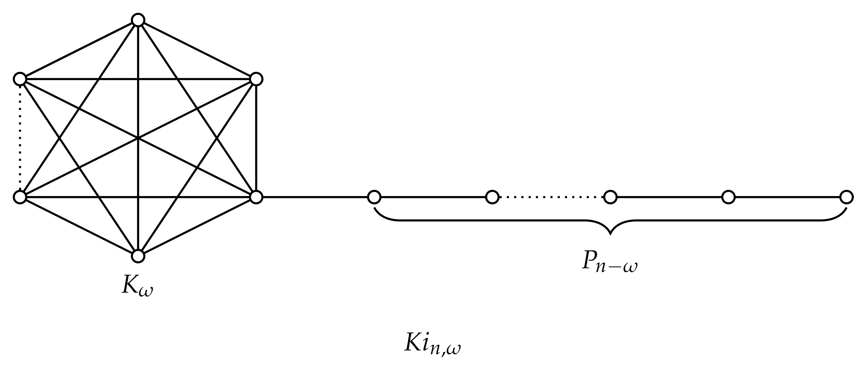
Figure 2.
The short kite graph .

Publisher’s Note: MDPI stays neutral with regard to jurisdictional claims in published maps and institutional affiliations. |
© 2021 by the authors. Licensee MDPI, Basel, Switzerland. This article is an open access article distributed under the terms and conditions of the Creative Commons Attribution (CC BY) license (https://creativecommons.org/licenses/by/4.0/).
Share and Cite
MDPI and ACS Style
Das, K.C.; Shang, Y. Some Extremal Graphs with Respect to Sombor Index. Mathematics 2021, 9, 1202. https://doi.org/10.3390/math9111202
AMA Style
Das KC, Shang Y. Some Extremal Graphs with Respect to Sombor Index. Mathematics. 2021; 9(11):1202. https://doi.org/10.3390/math9111202
Chicago/Turabian StyleDas, Kinkar Chandra, and Yilun Shang. 2021. "Some Extremal Graphs with Respect to Sombor Index" Mathematics 9, no. 11: 1202. https://doi.org/10.3390/math9111202
Note that from the first issue of 2016, this journal uses article numbers instead of page numbers. See further details here.