Abstract
In this paper, two new distributions were introduced to model unimodal and/or bimodal data. The first distribution, which was obtained by applying a simple transformation to a unit-Birnbaum–Saunders random variable, is useful for modeling data with positive support, while the second is appropriate for fitting data on the (0,1) interval. Extensions to regression models were also studied in this work, and statistical inference was performed from a classical perspective by using the maximum likelihood method. A small simulation study is presented to evaluate the benefits of the maximum likelihood estimates of the parameters. Finally, two applications to real data sets are reported to illustrate the developed methodology.
1. Introduction
The Birnbaum–Saunders (BS) distribution has been used principally for modeling the lifetime of certain structures under dynamic load, and it was introduced by Birnbaum and Saunders [1]. The probability density function (pdf) of the BS distribution is given by:
where is the pdf of the normal distribution and , where is a shape parameter and is a scale parameter. We use the notation . The BS model has been extended to a large number of families of distributions. Castillo et al. [2], for example, introduced the epsilon Birnbaum–Saunders family of distributions based on the epsilon-skew-symmetric distribution, while Vilca-Labra and Leiva-Sánchez [3] proposed a new fatigue model from the skew-elliptical family of distributions. The new proposal is called the doubly generalized Birnbaum–Saunders distribution, and within its main properties, it is highlighted that the incorporation of the elliptical aspect allows the kurtosis to be flexible and that the skewness makes the asymmetry flexible. Martínez-Flórez et al. [4] introduced the asymmetric alpha-power extension of the BS model. A generalization referred to as the proportional hazard Birnbaum–Saunders distribution was studied by Moreno-Arenas et al. [5], which includes a new parameter that provides more flexibility in terms of skewness and kurtosis. The BS model also has been used in the study of linear regression models as in Rieck and Nedelman [6], where it was supposed that with for and the errors in the linear model have a sinh-normal (SHN) distribution with parameter vector . Santos and Cribari-Neto [7] numerically evaluated the finite sample performances of the likelihood ratio, score, and Wald tests in the log-Birnbaum–Saunders regression model and introduced a RESET-like misspecification test for the proposed model by Rieck and Nedelman [6]. Furthermore, Balakrishnan and Zhu [8] discussed the maximum likelihood estimation of the model parameters under a log-linear link function for the BS lifetime regression model with equal and unequal shape parameters.
The pdf of the SHN model is given by:
where is a shape parameter, is a location parameter, and is a scale parameter. A random variable Y following the model in (2) is denoted by .
The SHN model was extended by Barros et al. [9] by considering a Student t distribution for the errors. This proposed Student t log-BS regression model allows attenuating the influence of the outlying observations. Other extensions of the SHN model were considered by Leiva et al. [10] and Santana et al. [11].
Generalizations of the BS distribution to model data with support in the interval (0, 1) have also been considered by several authors. Mazucheli et al. [12] presented a type of BS distribution with support in the interval , which became a new alternative to the beta and Kumaraswamy distributions. This new proposal is called the unit-Birnbaum–Saunders (UBS) model and has the pdf given by:
where , is a shape parameter and is a scale parameter.
To explain response variables between zero and one, such as proportions or rates, alternative statistical models to the beta regression model were studied by Martínez-Flórez et al. [13]. The beta regression model is useful to study relations between variables where the response corresponds to rates, proportions, or indexes. Among the several studies related to the issue, we have Ospina et al. [14], Simas et al. [15], Rocha and Simas [16] and Cribari-Neto and Souza [17], among others. Recent applications of the beta regression model can be found in Ghosh [18], who developed the robust minimum density power divergence estimator and a class of robust Wald-type tests for the beta regression model. For the applications, the author considered data on health measurements of several athletes collected at the Australian Institute of Sport (HIV data) and data on anxiety, depression, and stress in non-clinical women in Australia (stress-anxiety data). On the other hand, Kim et al. [19] proposed control charts of mean and variance by using a copula Markov statistical process control (SPC) and a conditional distribution with diverse copula functions. The authors used beta regression to explain the behavior of the average run lengths of the control charts of conditional variance with data on Major League Baseball (MLB) batting average (BA) and earned run average (ERA) data from the 1998 to 2016 seasons. The main objective of this work is to introduce new families of distributions capable of modeling bimodal data with positive support or on the unit interval. The extension to the case of regression models is also studied.
The rest of this paper is organized as follows: Section 2 introduces the non-negative sinh-normal distribution, and its main statistical properties are studied in detail. The log-sinh-normal regression model is also studied. In Section 3, the log-sinh-normal regression model is introduced, and its main properties are discussed. Section 4 presents the normal distribution, and its respective extension to the case of regression models is studied. In Section 5, a small Monte Carlo simulation study is presented. Finally, in Section 6, two real data applications are reported and compared with several rival models.
2. Non-Negative Sinh-Normal Distribution
In this section, a new non-negative distribution is introduced, which is obtained by extension of the UBS model. Let X be a random variable following a UBS distribution. If , then the distribution of Y has positive support and is referred to as a non-negative sinh-normal (SHN) distribution. The pdf of the non-negative SHN model is given by:
where is the pdf of the standard normal distribution. The distribution in (4) can also be called log-unit-Birnbaum–Saunders (LUBS). One can see that a more general form of the non-negative SHN model is given by the pdf:
where , , , and are the parameters of the shape, location, and scale, respectively. This model is denoted by , and we refer to it as the log-sinh-normal model.
The density function in Equation (5) integrates to one, and the proof of this can be seen in Appendix A. Figure 1 displays some forms of the pdf of the LSHN distribution for selected values of , , and . One can see in Figure 1a that the LSHN density is unimodal for , whereas for , the LSHN density is bimodal (see Figure 1b). This is a great result since it is possible to have a distribution for positive bimodal data.
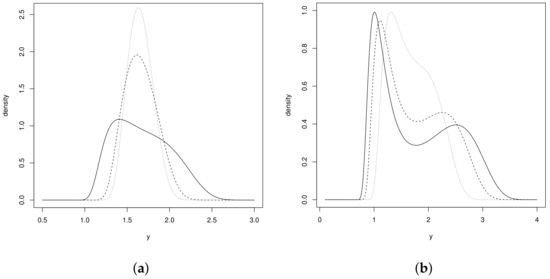
Figure 1.
Probability density function of the distribution for: (a) (solid line), (dashed line), and (dotted line); (b) (solid line), (dashed line), and (dotted line).
2.1. Distribution Function, Survival Function, and Hazard Function of the LSHN Model
The cumulative distribution function (cdf) of the LSHN model is given by:
where is the cdf of the SHN distribution. It follows from (5) and (6) that the survival and hazard functions are given, respectively, by:
and:
where and are the survival and hazard functions of the SHN model. The graphs in Figure 2 show the form of the hazard function for some selected values of the parameters. The plots reveal that the LSHN density increases up to a certain value and then decreases to zero.
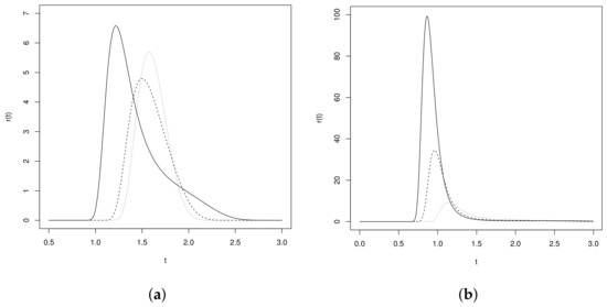
Figure 2.
Hazard function of the distribution for: (a) (solid line), (dashed line), and (dotted line); (b) (solid line), (dashed line), and (dotted line).
2.2. Moments of the LSHN Model
It can be shown that the r-th moment of the random variable Y following a distribution is given by:
where is the moment-generating function (mgf) of the random variable with the SHN distribution. Following some results found by Rieck [20], we have that:
where , , and is the third-order Besser function defined by:
For the special case of (the LUBS model), one can prove that:
and:
From the above results, it can be concluded that the LSHN distribution can be obtained by applying the transformation to a random variable .
2.3. Cumulant-Generating Function and Mode
Let with , then the random variable Y has an LSHN distribution. It follows that:
Letting , for , and following Mazucheli et al. [21], we have:
Now, the cumulant-generating function (cgf) is given by:
where is the j-th moment of the random variable Y. We have that,
The modes of the LSHN distribution can be obtained by maximizing the logarithm of the pdf. Thus, let and in the logarithm of the pdf of the LSHN model; taking the derivative and setting the resulting derivative equal to zero, it is obtained that the mode (or modes) of the pdf of the LSHN distribution is (are) the solution(s) of the non-linear equation:
Solving this non-linear equation, the mode(s) of the LSHN distribution is (are) found.
2.4. Asymptotic Distribution
If , it can be proven that the random variable converges to a normal distribution when , that is random variable Y converges to a log-normal (LN) distribution when . Therefore, it follows from (6) that, if , then:
Thus, if , then:
where is the inverse function of the function.
3. The LSHN Regression Model
Regression models have been a statistical technique widely used in many areas of knowledge to explain the behavior of a response variable, say Y, as a function of other variables called explanatory variables, say , and a vector of unknown parameters called regression coefficients, which is denoted by . In this section, the LSHN linear regression model is introduced by considering a random sample of variables , such that:
for , with and . In this case, we suppose the functional relationship:
where the random variables for .
The functional relationship in Equation (11) is justified below from Theorem 1.
Theorem 1.
Let , then for , has a distribution.
Proof.
Consider , and let , then and ; thus:
That is, . □
To construct the model, we considered a random sample , such that for ; and we supposed that and for where . Letting and since (this follows from Theorem 1), taking where , we have that, , that is .
Thus, for , we have that,
Now, for , it follows that , then , and then:
It can be seen from the previous result that the regression model given in (10) generalizes the obtained model from Theorem 1.
3.1. Maximum Likelihood Estimation in the LSHN Regression Model
To get the estimates of the parameters in the LSHN regression model, we considered the maximum likelihood method. Thus, given a random sample of size n, say , where , the log-likelihood function for the parameter vector can be written as follows:
where and for .
After taking partial derivatives of the log-likelihood function (12) with respect to the parameters of interest and setting them equal to zero, we obtain the following score equations:
where , for . The maximum likelihood estimators for and , are the solutions to the equations , , and , which require a numerical method, such as the Newton–Raphson or quasi-Newton.
3.2. Observed and Expected Information Matrix
The elements of the observed information matrix for the parameter vector , which are denoted by with , can be obtained by calculating the second partial derivative of the log-likelihood function (12), i.e., . These elements are given by:
The previous results are similar to those obtained by Rieck and Nedelman [6]. The elements of the expected information matrix, , defined as times the expected values of the elements of the observed information matrix, are denoted by , , , , , and . Following Rieck and Nedelman [6], we make:
Then, the following elements of the matrix are obtained:
where:
and is the error function given by:
One can be show that , that is the information matrix is non-singular, which guarantees the existence of the covariance matrix of the maximum likelihood estimators. The Fisher information matrix is given by . The existence of also guarantees that the vector of maximum likelihood estimators has asymptotic distribution:
that is the maximum likelihood estimators of the model parameters are consistent and asymptotically follow a normal distribution with the covariance matrix being the inverse of the Fisher information matrix. The approximation can be used to construct confidence intervals for the parameters . These confidence intervals are given by:
where corresponds to the square root of the r-th diagonal element of the matrix and denotes the quantile of the standard normal distribution.
4. Unit-Sinh-Normal Distribution
Now, we introduce the SHN model with support on interval , which is denominated by the unit-sinh-normal model, and it is denoted by . The pdf is given by:
where , is a shape parameter, is a location parameter, and is a scale parameter. It can be seen in the complement of the sinh and cosh functions that the density function in (16) is defined on the log-log complementary transformation, which is widely used in generalized linear models. Although the density (16) could be defined from the log-log link function, we used the log-log complement link function. Note that, if , then , and the simple transformation leads to the model with the log-log link function. Figure 3 displays some plots of the pdf of the USHN distribution for some selected values of the parameters. The plots reveal that the USHN density is unimodal for (see Figure 3a), and the density function is bimodal for (see Figure 3b). One of the advantages of the USHN distribution is that it can be used for modeling data sets of proportions and rates with bimodal behaviors.
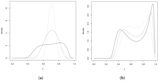
Figure 3.
Probability density function of the distribution for: (a) (solid line), (dashed line), and (dotted line); (b) (solid line), (dashed line), and (dotted line).
4.1. Distribution Function, Survival Function, and Hazard Function of the USHN Model
Is easy to see that the corresponding cdf of the random variable is given by:
where is the cdf of the distribution. The survival function and hazard function are given by:
and:
respectively, where and are the survival function and hazard function of the SHN model, respectively. From (17), it is concluded that:
which implies that . Figure 4 shows the behavior of the hazard function of a USHN random variable for some selected values of the parameters. The graphs reveal that the hazard function is increasing up to a certain value and then is decreasing to zero.
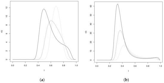
Figure 4.
Hazard function of the distribution for: (a) (solid line), (dashed line), and (dotted line); (b) (solid line), (dashed line), and (dotted line).
One can see that a random variable Y following a distribution can be generated by using the expression:
where denotes the uniform distribution on the interval and refers to the inverse of the cdf of the standard normal distribution.
4.2. Moments of the USHN Model
The r-th moment of a random variable Y following a distribution is given by:
where . Using the Taylor expansion for and from the r-th moment of the distribution, it follows that:
where and , with the third-order Besser function defined in (7).
4.3. Cumulant-Generating Function and Mode
The mgf of the USHN model can be obtained by using:
where and , with being the mgf of the UBS distribution. Thus,
where is the cgf of the UBS distribution. To find the mode of the USHN distribution, we reasoned in the same way as in the LSHN model. Then, let and . Deriving the logarithm of the pdf of the USHN distribution, substituting and , and equaling to zero, we obtain the non-linear equation:
Solving this non-linear equation, the mode(s) of the USHN distribution is (are) found.
4.4. Asymptotic Distribution
Let . One can prove that random variable converges to a normal distribution when tends to zero. Thus, if , then:
It follows from the result above that:
4.5. The LUSHN Regression Model
Now, we introduce the LUSHN linear regression model. We considered a set of p explanatory variables, which are denoted by , and a p-dimensional vector of unknown parameters , such that, for , it follows the functional relationship:
where . From (18), we have that,
hence, Thus, and therefore,
To obtain the estimates of the model parameters, we considered the maximum likelihood method as in the LSHN regression model. Thus, given a random sample of size n, say , the log-likelihood function for the parameter vector is given by:
where:
for .
The score function and the observed information matrix of the LUSHN regression model have the same form as the respective expressions of the LSHN regression model by substituting by and by defining:
for . The MLEs for , , and , are the solutions to the equations , and , which require a numerical method such as the Newton–Raphson or quasi-Newton.
5. Simulation Study
To analyze the behavior of the estimators of the parameters in the LSHN regression model, we carried out a small Monte Carlo simulation study. To generate the random variable USHN, we applied the described algorithm in this paper. In this simulation study, we analyzed the behavior of the estimators of the model parameters:
where . The values of the explanatory variable X were taken from a uniform random variable on the (0,1) interval, that is . Without loss of generality, we took the value of the scale parameter equal to ; however, the following results can be obtained for any value of the scale parameter from the simple transformation with . The values of shape parameter were taken as = 0.50, 0.75, 1.25, 1.75, 2.25, 2.75 to take into account different configurations in the form of the pdf of the random variable . On the other hand, since the coefficients , in the model (18) can be any number in the set of real numbers and there are no restrictions on the values that can be assumed, we took the particular values and . To analyze some statistical measures of the maximum likelihood estimator (MLE), we considered small, moderate, and large sample sizes: , and 5000 iterations were performed for each scenario. The studied characteristics were: the relative bias (RB), the root of the mean squared error (RMSE), and the ratio between the standard deviation (SD) of the estimate and the average SD (RSD). Finally, we examined the coverage probability (CP) of the 95% confidence interval based on the asymptotic normality of the ML estimators.
Table 1 and Table 2 present the results of the simulation study. It can be observed that the RB and RMSE of the MLEs tend to decrease when the sample size increases, which guarantees the unbiasedness and asymptotic consistency of the MLE. It is also observed that, for small sample sizes, important biases are obtained in the estimates of and . It is also observed that, for small sample sizes, important biases are obtained in the estimates of and . Another interesting aspect to take into account is that, for values less than one of the parameter, the bias of is quite considerable for small sample sizes; however, this bias is quite negligible for values of above of one.

Table 1.
Empirical relative bias (RB), root of the mean squared error (RMSE), ratio between the standard deviation of the estimate and the average standard deviation (RSD), and coverage probability (CP) of the 95% confidence interval for the MLEs of the and in the LUBS model.
Table 2.
Empirical relative bias (RB), root of the mean squared error (RMSE), ratio between the standard deviation of the estimate and the average standard deviation (RSD), and coverage probability (CP) of the 95% confidence interval for the MLEs of the and in the LUBS model.
Regarding the coverage rates of the confidence intervals (CP), the simulation results showed that these were higher than 95% for the parameter in all of the considered sample sizes. For the scale parameter , the CPs were low when there were small sample sizes (less than 50), and they tended to increase when the sample size increased to around 90 %. It was also observed that the CPs for the coefficients and were close to 95 % for moderate and large sample sizes (greater than 75).
6. Applications
To illustrate the potentiality of the proposed distributions, we considered two data sets of real-life examples taken from the literature. The first data set was an example of positive data called fatigue data in hardened steel. The second data set corresponded to data of the body fat data in athletes of the Australian Institute of Sport (AIS), which is an example of the observations on the interval.
6.1. Fatigue Data
This data set consisted of failure times in rolling contact fatigue of ten hardened steel specimens tested at each of the four values of four contact stress points, X. The data were obtained using a four-ball rolling contact test rig at the Princeton Laboratories of Mobil Research and Development Co. This data set was analyzed by Chan et al. [22] by considering the regression model:
We considered that the positive response variable T followed the distribution:
For this data set, we fit the log-BS (LBS) model, the log-skewed BS (LSBS) of Lemonte [23], and the proposed LSHN distribution. The MLEs of the parameters of the fitted models are given in Table 3.
Table 3.
MLE (standard error) for the LBS, LSBS, and LSHN models.
To compare the fitted models, we used the AIC and BIC criteria, which are given by:
where p is the number of parameters of the model in question and n is the sample size. The best model is the one with the smallest AIC or BIC. According to AIC and BIC criteria in the table, we can see that the asymmetric models LSBS and LSHN fit better than the LBS model, that is the data present a larger degree of asymmetry than allowed by the BS model. We can conclude that the regression model with the LSHN error distribution provides a better fit than the regression model with the LSBS error distribution.
The significance of the variable on the response variable can be tested through the Wald statistic, , which gives the value with the respective p-value , in such a way that the logarithm of contact stress points affects the failure time of the hardened steel.
We recall that if , then:
for . Figure 5b plots the envelope of the random variable . The plot reveals that the LSHN regression model presents a good fit to the Fatigue data. The plot in Figure 5a depicts the envelope for the log-BS model regression.
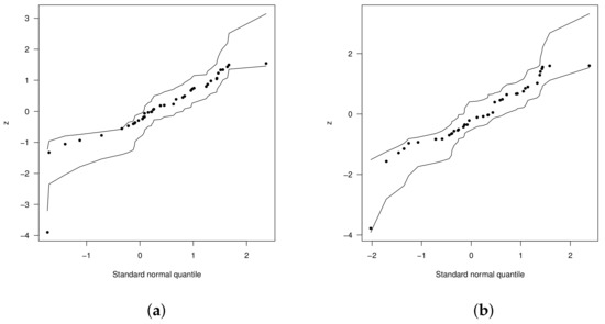
Figure 5.
Envelopes of the residuals for: (a) the LBS distribution and (b) the LSHN distribution.
6.2. Body Fat Data
We considered the data set included in the library sn of R Development Core Team [24] available for download at http://azzalini.stat.unipd.it/SN/index.html (accessed on 20 March 2021). We considered only the data of 37 rowing athletes in the AIS dataset. We were interested in the prediction of the body fat percentage (Bfat) of each athlete by considering their lean body mass (lbm). For the analysis, we considered the random variable:
where is the body fat percentage of the i-th athlete for . We also fit the beta regression model with logit link and the natural logarithm link to model the dispersion parameter. The MLEs of the parameters and their corresponding standard errors (in parenthesis) were: for the beta regression model, , , and with and ; for the LUSHN regression model, , , , and , with and . According to AIC and BIC criteria, the better model was the non-negative SHN. Figure 6 plots the envelope of the variable in which we can see that the LUSHN regression model presents a good fit to the body fat data.
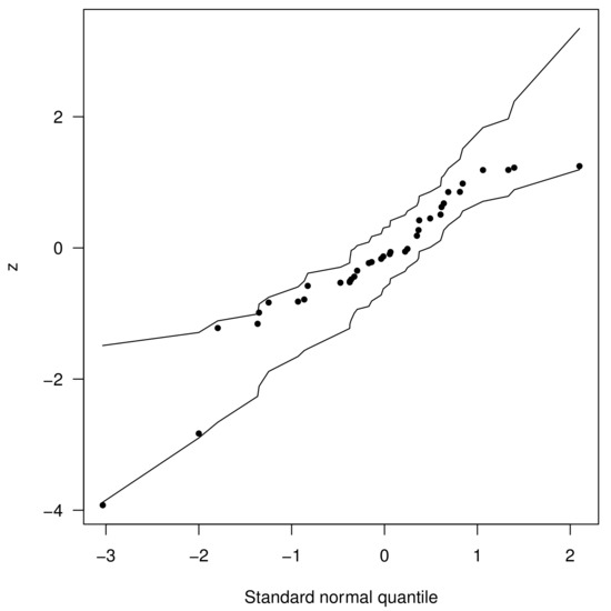
Figure 6.
Envelope of the residuals for the LUSHN regression model.
7. Conclusions
In this paper, two new families of bimodal distributions were introduced. The new families were generated by applying transformations to the unit-Birnbaum–Saunders and were very useful alternatives for modeling data limited on the interval (0,1) or with positive support, due to their flexibility to fit data with a high degree of asymmetry and/or kurtosis. The main statistical properties of the families and the problem of the parameter estimation were studied in detail by using the maximum likelihood method. The observed and expected information matrix for the family was also deduced. A small Monte Carlo simulation was carried out, showing that the maximum likelihood estimators had good asymptotic properties for moderate and large sample sizes. Extensions to regression models were also presented based on the new family of distribution. Furthermore, we showed that such families of distributions can be useful to fit better to real data sets, especially when the variables are considered to explain the response variable in a regression model.
Author Contributions
All authors contributed equally to this work. All authors read and agreed to the published version of the manuscript.
Funding
The research of R.T.-F. and G.M.-F. were supported by project: Resolución de Problemas de Situaciones Reales Usando Análisis Estadístico a través del Modelamiento Multidimensional de Tasas y Proporciones; Esquemas de Monitoreamiento para Datos Asimétricos no Normales y una Estrategia Didáctica para el Desarrollo del Pensamiento Lógico-Matemático. Universidad de Córdoba, Colombia, Code FCB-05-19.
Institutional Review Board Statement
Not applicable.
Informed Consent Statement
Not applicable.
Data Availability Statement
Details about data available are given in Section 6.
Acknowledgments
G.M.-F. and R.T.-F. acknowledges the support given by Universidad de Córdoba, Montería, Colombia.
Conflicts of Interest
The authors declare no conflict of interes.
Appendix A. Related Theorems
Theorem A1.
Let . Then, , where .
Proof.
The density of a Birnbaum–Saunders distribution is:
where is the pdf of the normal distribution and .
Letting , then , and by applying the theorem for the transformation of random variables, it follows that:
Thus, . □
Proposition A1.
The density function in Equation (5) integrates to one.
Proof.
We considered the density function such as:
and we let:
then,
□
References
- Birnbaum, Z.W.; Saunders, S.C. A new family of life distributions. J. Appl. Prob. 1969, 6, 319–327. [Google Scholar] [CrossRef]
- Castillo, N.O.; Gómez, H.W.; Bolfarine, H. Epsilon Birnbaum–Saunders distribution family: Properties and inference. Stat. Pap. 2011, 52, 871–883. [Google Scholar] [CrossRef]
- Vilca-Labra, F.; Leiva-Sánchez, V. A new fatigue life model based on the family of skew-elliptical distributions. Commun. Stat. Theory Methods 2006, 35, 229–244. [Google Scholar] [CrossRef]
- Martínez-Flórez, G.; Bolfarine, H.; Gómez, H.W. An alpha-power extension for the Birnbaum–Saunders distribution. Stat. Am. J. Theor. Appl. Stat. 2014, 48, 896–912. [Google Scholar]
- Moreno-Arenas, G.; Martínez-Flórez, G.; Barrera-Causil, C. Proportional Hazard Birnbaum–Saunders distribution with application to the survival data analysis. Rev. Colomb. Estad. 2016, 39, 129–147. [Google Scholar] [CrossRef]
- Rieck, J.R.; Nedelman, J.R. A log-linear model for the Birnbaum–Saunders distribution. Technometrics 1991, 33, 51–60. [Google Scholar]
- Santos, J.; Cribari-Neto, F. Hypothesis testing in log-Birnbaum–Saunders regressions. Commun. Stat. Simul. Comput. 2017, 46, 3990–4003. [Google Scholar] [CrossRef]
- Balakrishnan, N.; Zhu, X. Inference for the Birnbaum–Saunders Lifetime Regression Model with Applications. Commun. Stat. Simul. Comput. 2015, 48, 2073–2100. [Google Scholar] [CrossRef]
- Barros, M.; Paula, G.A.; Leiva, V. A new class of survival regression models with heavy-tailed errors: Robustness and diagnostics. Lifetime Data Anal. 2008, 14, 316–332. [Google Scholar] [CrossRef]
- Leiva, V.; Vilca-Labra, F.; Balakrishnan, N.; Sanhueza, A. A skewed sinh-normal distribution and its properties and application to air pollution. Commun. Stat. Theory Methods 2010, 39, 426–443. [Google Scholar] [CrossRef]
- Santana, L.; Vilca, F.; Leiva, V. Influence analysis in skew-Birnbaum–Saunders regression models and applications. J. Appl. Stat. 2011, 38, 1633–1649. [Google Scholar] [CrossRef]
- Mazucheli, J.; Menezes, A.; Dey, S. The unit-Birnbaum–Saunders distribution with applications. Chil. J. Stat. 2018, 9, 47–57. [Google Scholar]
- Martínez-Flórez, G.; Bolfarine, H.; Gómez, H.W. Power-models for proportions with zero/one excess. Appl. Math. Inf. Sci. 2018, 12, 293–303. [Google Scholar] [CrossRef]
- Ospina, R.; Cribari-Neto, F.; Vasconcellos, K.L.P. Improved point and interval estimation for a beta regression model. Comput. Stat. Data Anal. 2006, 51, 960–981. [Google Scholar] [CrossRef]
- Simas, A.B.; Barreto-Souza, W.; Rocha, A.V. Improved estimators for a general class of beta regression models. Comput. Statist. Data Anal. 2010, 54, 348–366. [Google Scholar] [CrossRef]
- Rocha, A.V.; Simas, A.B. Influence diagnostics in a general class of beta regression models. Test 2011, 20, 95–119. [Google Scholar] [CrossRef]
- Cribari-Neto, F.; Souza, T.C. Testing inference in variable dispersion beta regressions. J. Stat. Comput. Sim. 2012, 82, 1827–1843. [Google Scholar] [CrossRef]
- Ghosh, A. Robust inference under the beta regression model with application to health care studies. Stat. Methods Med. Res. 2019, 28, 871–888. [Google Scholar] [CrossRef] [PubMed]
- Kim, J.M.; Baik, J.; Reller, M. Control charts of mean and variance using copula Markov SPC and conditional distribution by copula. Commun. Stat. Simul. Comput. 2021, 50, 85–102. [Google Scholar] [CrossRef]
- Rieck, J.R. Statistical Analysis for the Birnbaum–Saunders Fatigue Life Distribution. Ph.D. Thesis, Department of Mathematical Sciences, Clemson University, Clemson, SC, USA, 1989. [Google Scholar]
- Mazucheli, J.; Leiva, V.; Alves, B.; Menezes, A.F.B. A new quantile Regression for modeling bounded data under a unit Birnbaum–Saunders distribution with applications in medicine and politics. Symmetry 2021, 13, 682. [Google Scholar] [CrossRef]
- Chan, P.S.; Ng, H.K.T.; Balakrishnan, N.; Zhou, Q. Point and interval estimation for extreme-value regression model under Type-II censoring. Comput. Stat. Data Anal. 2012, 52, 4040–4058. [Google Scholar] [CrossRef]
- Lemonte, A.J. A log-Birnbaum–Saunders regression model with asymmetric errors. J. Stat. Comput. Simul. 2012, 82, 1775–1787. [Google Scholar] [CrossRef]
- R Development Core Team. R: A Language and Environment for Statistical Computing; R Foundation for Statistical Computing: Vienna, Austria, 2018; Available online: http://www.R-project.org (accessed on 22 February 2021).


Publisher’s Note: MDPI stays neutral with regard to jurisdictional claims in published maps and institutional affiliations. |
© 2021 by the authors. Licensee MDPI, Basel, Switzerland. This article is an open access article distributed under the terms and conditions of the Creative Commons Attribution (CC BY) license (https://creativecommons.org/licenses/by/4.0/).