Abstract
Healthy eating is an essential element to prevent obesity that will lead to chronic diseases. Despite numerous efforts to promote the awareness of healthy food consumption, the obesity rate has been increased in the past few years. An automated food recognition system is needed to serve as a fundamental source of information for promoting a balanced diet and assisting users to understand their meal consumption. In this paper, we propose a novel Lightweight Neural Architecture Search (LNAS) model to self-generate a thin Convolutional Neural Network (CNN) that can be executed on mobile devices with limited processing power. LNAS has a sophisticated search space and modern search strategy to design a child model with reinforcement learning. Extensive experiments have been conducted to evaluate the model generated by LNAS, namely LNAS-NET. The experimental result shows that the proposed LNAS-NET outperformed the state-of-the-art lightweight models in terms of training speed and accuracy metric. Those experiments indicate the effectiveness of LNAS without sacrificing the model performance. It provides a good direction to move toward the era of AutoML and mobile-friendly neural model design.
1. Introduction
According to the World Health Organization (WHO), 39% of adults aged 18 years old and above were overweight and 13% were obese in 2016. There are a few factors associated with the increasing number of overweight and obese people, such as less exercise, stress level, and meal consumption. Among them, the most prominent factor is the significant shift of eating habits with an unhealthy pattern of food consumption [1]. Numerous researches evidently show a healthy and balanced diet intake has a major influence to prevent obesity. In the long term, obesity often will lead to chronic diseases, for example, type 2 diabetes and coronary heart disease.
Several reporting platforms were created to facilitate the dietary assessment and increase the awareness of healthy food consumption such as the Nutrition Data System for Research (NDSR) and Diet In Nutrient Out (DINO) [2,3]. Users can input the food category and portion of their dietary intake into the system. Training is required for users to learn how to provide the manual data entry to describe the food in a precise manner. If the provided information is not clear, further interaction with a dietitian is required to capture the detailed information of dietary intake. Although this has been proven to be helpful, it is not cost-effective and time-consuming for both the end-user and the dietitian to manually provide or review the dietary intake. To get rid of manual input by end-users, some image-based dietary assessments have been implemented to improve user-friendliness. It allows users to capture their food photos directly and upload to different discussion channels such as social media or mobile applications. Based on the digital food images, the dietitian can provide professional feedback to the user [4]. This method is designed to minimize the learning barrier for the end-user, but the scalability is constrained by the number of dietitians in a team.
1.1. Model Scaling for Convolutional Neural Network
The rapid development of deep learning has surpassed human-level performance when performing image classification. Convolutional Neural Network (CNN) is superior at automatically recognizing the image features to deliver high accuracy in image classification [5]. It can be used to automate the process of food recognition with digital images. Several CNN models were proposed to improve the automation of self-reporting dietary platforms with various designs of network architectures [6]. While preliminary results are promising with deep neural networks, expensive computation power to implement the deep CNN makes it difficult to be widely used. It is not feasible to run the deep CNN on edge devices. Furthermore, it takes an extremely long period of time to train the deep CNN for a large dataset. It can take more than a week to train on a professional level GPU [7].
Typically, the accuracy of the CNN model improves when it has a more complicated and deeper architecture. Adding a new layer or increase the parameter size is the common approach to handle a bigger dataset. Hierarchical decomposition in the deeper layers helps extract a rich set of image features. However, the number of parameters in a CNN is not always proportional to the model performance [8]. A deeper CNN has become harder to scale further due to the inefficient performance gain and exponential growth of computational complexity. Instead of expanding the model depth, researchers have started to redesign the convolution function. Depth-wise separable convolution was first introduced by Inception and subsequently used by MobileNet to diminish the model size yet deliver excellent performance. In conventional convolution, the complexity of a layer can be calculated as , where is the two-dimensional kernel size, is the number of the input channel, is the size of the input image, and is the number of the output channel. Depth-wise separable convolution consists of depth-wise convolution to ingest each input channel into a single convolution separately, then followed by a 1 × 1 pointwise convolution to combine the extracted features [9]. The number of operations can be formulated as . It helps reduce the number of parameters (up to eight times fewer parameters), while still retaining a similar performance.
The inspiration from MobileNet has pushed the development of the lightweight model to become a trending research topic. Group convolution and channel shuffle operation were introduced in SuffleNet to highly reduce the computational time. Group convolution helps split the input channels into different chunks for multiple convolution groups. It can be interpreted as , where is the number of convolution groups [10]. Given , and , it is able to lower the computational cost by a factor of three. By having more groups, the training time can be further reduced. Subsequently, Ido Freeman et al. proposed spatial separable convolution in EffNet to refine the depth-wise separable convolution with a line kernel, separable pooling, and a column kernel. The computational cost is only half of the normal depth-wise operation [11]. Figure 1 visualizes the convolution design in MobileNet, ShuffleNet, and EffNet.
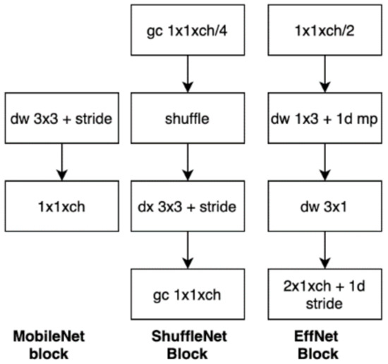
Figure 1.
Convolution design for MobileNet, ShuffleNet, and EffNet.
1.2. Neural Architecture Search
Although researchers have made a huge progress in developing the cost-effective CNN model, it is time-consuming to conduct model-based experiments repeatedly to search for the best settings. Recently, Neural Architecture Search (NAS) has become an emerging field to leverage the concept of AutoML. It was pioneered by Zoph et al. to automate the process of building the model architecture [12]. It involves a Reinforcement Learning (RL) controller for searching for the best child model architecture within its search space. The RL-based controller is a Recurrent Neural Network (RNN) that proposes a list of sequential layers to construct a neural network for its child model. In the context of image classification, the child model will be CNN. NAS has been proven to deliver effective models that are able to outperform hand-crafted models designed by human experts in a painstaking process. However, there are few limitations in the existing NAS approaches. Firstly, the search strategy in classic NAS is inefficient and exceedingly longer GPU hours are needed to converge for a reasonable child network. Efficient NAS (ENAS) is relatively faster in searching the child network, but it has a restricted search space for convolution cells such as separable convolution and identity convolution only [13].
In this paper, we propose a novel approach of NAS, namely Lightweight-NAS (LNAS) to generate a mobile-friendly CNN model for food image classification. LNAS utilizes weight sharing among the child candidates to speed up the convergence process. Similar to transfer learning, LNAS allows the weights to be transferred between child models to avoid the need of training from scratch when proposing a new child model. LNAS extends the search space with more advanced convolution functions such as the Inverted Residual Unit. This allows the child model to be composed with a set of convolutional blocks that are optimized for efficiency and performance.
The contribution of this paper can be summarized as follows: (1) Authors propose a novel lightweight neural architecture search with weights sharing and an advanced search space. It refines the constrained search space in ENAS with sophisticated convolution functions and allows each layer to have its own search space to get rid of limitations in the ENAS. (2) The final CNN model produced by LNAS, namely LNAS-NET is able to deliver outstanding performance for image-based food classification. To the best of the authors’ knowledge, it is the first time to employ this NAS strategy specifically to perform classification for digital food images. Extensive experiments are conducted on open-source food datasets to demonstrate the performance gain between LNAS-NET and existing state-of-the-art thin models, such as MobileNet and ShuffleNet, and the experimental results demonstrate that our proposed method outperforms the state-of-the-art models.
2. Methodology
The high-level design of LNAS implements a two-steps training approach to improve the child models over multiple iterations. Firstly, the RNN controller selects a child model from its search space and computes the reward scores by using policy-based reinforcement learning [14]. In the second step, the selected child model is trained extensively to observe the performance over time. Once the accuracy of the child model has been evaluated, the trained weights will be retained inside the candidate pools and can be shared by the potential candidates. The RNN controller is set back to its first step to redesign the child model with its latest parameters. The two-step training is repeated for 300 iterations to obtain the final architecture of the child model. Figure 2 shows the process flow of LNAS.
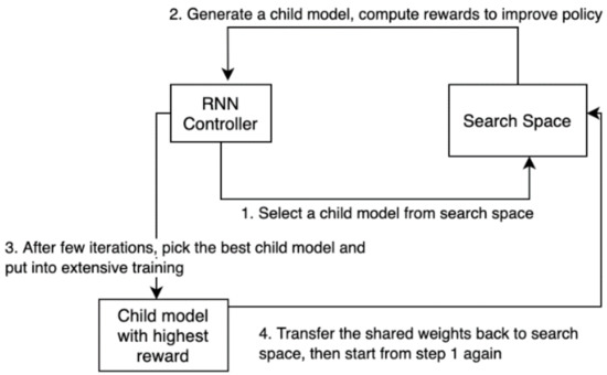
Figure 2.
Process flow of LNAS.
In this section, we first present the search space of LNAS. After that, we explain the search strategy to obtain the RNN controller weights and the shared weights of the child models.
2.1. Search Space
In LNAS, the search space can be represented as a directed acyclic graph (DAG). Instead of training the child model from scratch, whenever the RNN controller proposes a new child architecture, DAG is built to represent the complete connection in the entire search space. Essentially, each child model is a subgraph of the DAG. All vertexes in the previous layer are allowed to connect to any node in the following layer. The possible number of child models can be calculated as:
where is the number of nodes for each layer and is the number of layers in the DAG. It has 8 intermediate layers and 8 nodes per layer, which is equivalent to 16.77 million of potential sub-networks in the DAG.
By representing the entire search space as a DAG, it is possible to share the trained weights between the child models. Figure 3 shows the search space in DAG. The red arrow represents the activated connection to be included in the child model. Since the child model is a subgraph of DAG, the parameters of the child model can be transferred into DAG. This has been proven to deliver a much faster training speed than traditional NAS [15]. Unlike other NAS methods, DAG’s vertex in LNAS represents a stacked convolution block with multiple layers such as convolution, pooling, and batch normalization, rather than just a single layer in the child model. LNAS has three convolution blocks in the search space, namely Residual Unit, Bottleneck Residual Unit, and Inverted Residual Unit.
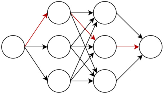
Figure 3.
Directed acyclic graph to represent LNAS’s search space.
A residual unit was firstly proposed in ResNet to implement identity mapping with the concept of skip connection. Each unit comprises two identical convolution layers and two batch normalization layers. Before entering the residual unit, the shortcut connection is created to sum the output of the previous block with the output of the current block. This helps preserve the image features in the deeper network as well as minimize the impact of a vanishing gradient [16]. In the residual unit, the convolution layer can be formulated as:
where is the kernel with dimension and is the input from the previous layer. The kernel size is 3 × 3 in a typical residual unit to form a symmetric shape from an odd-sized square.
The weights of the convolution layer are continuously evolving during the backpropagation training. When the propagation goes deeper, a minor change to the weights of the shallow layers can result in a large difference in a later state. Each layer has to constantly adapt to the new distribution, which is known as internal covariate shift [17]. Batch normalization can help approximately estimate the weight changes and maintain the same distribution in every training step. It normalizes the output of each layer in mini-batch processing and reduces the scale change of its previous layer. Batch normalization is expressed as:
Scale and shift are trained during the backpropagation process. This usually leads to a better generalization to the unseen image and reduces the error rate [18].
The output of batch normalization will be applied to the non-linear function to decide the activation status of each neuron. Nonlinearities support the CNN to learn the complex features that are not linearly separated. In this paper, a Rectified Linear Unit (ReLu) is used as the activation function of the convolution layer. It has a faster training speed and a better accuracy than the Hyperbolic Tangent Function (Tanh) in computer vision [19]. ReLu can be formulated as:
Derived from the residual unit, the bottleneck residual unit is a variant of residual design that shares the same concept with the residual unit. However, it has three convolution layers instead of two. The kernel sizes are 1 × 1, 3 × 3, and 1 × 1, respectively. The skip connection is formed to pass through a stack of 3 layers and carry out the matrix addition to compute the output. The benefit of the first 1 × 1 layer is to reduce the dimension of highly dense data; hence, 3 × 3 can operate on lower dimensions to extract the image features. Finally, the last layer restores the image to its original dimension. The intuition is to create an efficient convolution block and have fewer parameters [20]. However, some features might be discarded that lead to information loss during the dimensionality reduction. It can be used in conjunction with the residual unit to maximize the productivity of CNN.
To capture a complex representation of images without information loss, an inverted residual unit was proposed to incorporate depth-wise separable convolution and a linear bottleneck layer. The bottleneck residual unit follows a wide, narrow, and wide approach to arrange the sequence of stacked layers. Oppositely, the inverted residual unit implements the sequence of narrow, wide, and narrow to its layers instead of dimensionality reduction. The first l × 1 layer is responsible to expand the input features into a higher-dimensional space. The activation function ReLu6 is applied to encourage the learning of sparse features [21], which can be formulated as:
The output of ReLu6 is fed into a 3 × 3 depth-wise convolution layer. It has lower computational costs with the reduced number of parameters to achieve spatial filtering to the higher-dimensional input. The last 1 × 1 convolution layer helps map the spatially filtered features into a low-dimensional space. To further retain the learned features, the linear combination of the last layer is preserved without going through the activation function. This inverted structure greatly improves the training efficiency by reducing the mathematical operations to create a mobile-friendly neural network [22].
The search space of LNAS comprises three convolution blocks, as discussed above. Depending on the settings, each convolution block can have multiple nodes to represent the different variants in DAG. This is to augment the number of possible child models and leave the decision to LNAS. As mentioned previously, there are 16.77 million of possibilities in the search space to enhance the quality of child models. In the next section, we discuss how LNAS searches through the DAG to select the best possible child model.
2.2. Search Strategy
The central of LNAS’s search strategy is the RNN controller with 100 hidden LSTM units. The reason of choosing the recurrent model is to enable the controller to consider the previous steps and sequentially choose a child model within the DAG. The softmax function is applied to normalize the probability distribution of LSTM over all possible connections to the next vertex [23]. It can be explained as:
where is the LSTM input and is the number of possible connections to the next layer.
There are two sets of parameters to be learned for each iteration, namely the controller weights and the shared weights . During the first phase, we update the controller weights and leave the unchanged. The goal is to maximize the expected reward in the search process by using an RL-based framework. Reinforcement learning has two major types of frameworks which are value-based and policy-based methods. The value-based method estimates the optimal value function to determine the control policy, while the policy-based method directly learns the optimal policy without looking at the value function [24].
In this paper, we choose the REINFORCE algorithm to iteratively amend with the smooth update. It is a type of policy gradient method that updates the probability distribution of actions to increase the probability with higher expected reward, aiming to generate a better child model over time [25]. Compared to the value-based method, the policy-based method has a faster convergence speed and naturally fits into continuous high-dimensional data. The reward function is defined as:
The function is a stochastic policy for a set of state associated to actions that are parameterized by to define the strategy of the controller behavior. The stationary distribution of Markov chain’s states in respect of is denoted as . Finally, is the estimated reward of the state-action pair with respect to the policy . In Markov chain’s states, regardless of how the present state has arrived, the possible next steps are fixed [26]. For example, the probability of connecting to any future vertex in DAG is solely dependent on the state of the current step.
To train toward the optimal parameters, we need to use the gradient descent to estimate the gradient , then, iteratively update the with the goal of finding the best child model in the search space. To achieve this, REINFORCE collects a full trajectory by using its current policy, then updates the weights in a Monte Carlo style. It can be formulated as:
A trajectory is the sequential set of to reach the final state. The estimated reward of a trajectory is denoted as , where is the number of trajectories in a batch. The reward can be estimated by using the accuracy of a child model in these particular trajectories [27]. Notably, the accuracy is calculated on the validation set instead of the training set to prevent a high-biased model that leads to overfitting. The equation below is the mathematical expression of a single update step in our gradient descent. The step size defines the learning rate at each iteration.
The above equation estimated the unbiased gradient, but it has a relatively high variance. To minimize the variance between each update step, the baseline function is deployed as below:
computes the moving average baseline to reduce the variance with respect to the baseline decay and current reward . We amend the gradient method to subtract during the gradient update to prove an unbiased yet low-variance estimation of the gradient.
So far, we have discussed the first phase of the search strategy to update the controller weights. The output of the first phase is a child model with the highest reward. During the second phase, we fix the controller policy and retrain the child model to update its shared weights. We use the stochastic gradient descent (SGD), , as our optimization algorithm to update in a mini-batch fashion [28]. For each iteration, a mini-batch is sampled with examples from the training images. The gradient estimate is computed based on sampled images instead of the entire population. The samples are drawn in a uniform distribution. This is often applied to huge training data to fasten the training process.
Similar to the update step in the RNN controller, we need to update the weights with respect to the learning rate. However, the training at this phase has more iterations to ensure the network is able to capture the image features. To reduce overfitting into training data, cosine annealing is used as the learning rate schedule function. It starts with the large learning rate to approach the local optimum; then, it is swiftly decreased to the minimum threshold when it is closer to the local optimum. It is increased rapidly again at the first epoch of the next subgroup to jump out from the local optimum.
In the above equation, represents the number of epochs since the last restart. The index of the current epoch is denoted as . In contrast with a cold restart to use random numbers as a new starting point, the cosine annealing is more generalized to re-use the best learning rate from its previous epochs. It prevents the SGD to get trapped into the local minimum [29].
After the second phase, the shared weights are transferred to the DAG to allow weight sharing across all child models. It is possible to transfer the weights since the child model is essentially just a subgraph inside the DAG. We then trigger the RNN controller to update from the validation set and select the next child model based on its policy again. The process is repeated until the maximum number of batches, or the accuracy has reached the expected value. The child model at the last epoch is deemed as the best model for comparison purposes.
3. Experiments and Results
We run a two-phases training in LNAS for 300 epochs to obtain the final CNN model, namely LNAS-NET. Figure 4 shows the network architecture of LNAS-NET. It has a total of 8 convolution blocks for feature extraction and a fully connected layer for feature classification. To ensure our model is generalized well to unseen images, LNAS-NET is generated by using the CIFAR-100 data instead of food images [30]. In this section, LNAS-NET will be re-trained from scratch with two open-source data for food images, namely food-11 and food-101 [31]. Food-11 contains 11 major food categories with a total of 16,643 images. For food-101, it is much larger than food-101. It consists of 101 types of food labels, sums up to 101,000 labeled food images that cover multiple cruises. Both datasets are being split into 60% for training, 15% for validation, and 25% for testing. Comprehensive experiments are performed to compare the results of LNAS-NET with other state-of-the-art lightweight models, which are MobileNet, MobileNetV2, ShuffleNet, and ShuffleNetV2.
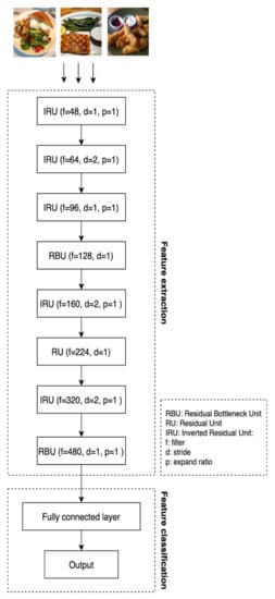
Figure 4.
Network architecture of LNAS-NET. It is the final child model designed by LNAS. LNAS-NET consists of 9 layers with 5 residual bottleneck units, 1 residual unit, 2 inverted residual units and 1 fully connected layer.
3.1. Settings
To have a fair comparison, the hyperparameters are the same for all models involved in the experiments. All models were trained with 200 epochs. SGD was chosen as an optimization method with 0.9 nesterov momentum and 0.0005 weight decay. The learning rate starts with 0.1 and reduces at milestones 60, 120, and 160 with a 0.2 multiplicative factor of learning rate decay. The images were resized into 150 × 150 before fed into the neural network. Image augmentation is applied to the dataset during training to reduce overfitting and increase diversity by using a label-preserving transformation [32].
To accelerate the training, all models were trained on the GPU machine, which is RTX2070 with 8GD of DDR6 VRAM. It is built on the Turing architecture with the base clock as 1410 MHz and 2304 CUDA cores [33]. For every model, the batch size of input images is set to fully utilize the VRAM. To observe the model performance over iterations, we have to estimate the loss value between the predicted labels and true labels. The cross- entropy loss function is used when adjusting model weights during training [34]. It is defined as:
where is the total number of class labels, is the true label, and is the predicted label. We use the loss value to measure the training performance and accuracy to measure the classification metric for the validation set and the test set.
3.2. Results
Figure 5a shows the loss value of the food-11 training dataset. The lower loss value indicates the smaller error rate between the predicted and actual value. For both datasets, the proposed LNAS-NET has constantly maintained a lower loss value and eventually reached the lowest loss value at the 200th epoch. It is noticeable that the proposed LNAS-NET has a faster convergence speed to arrive at a lower loss value within the first few epochs. On the other hand, the loss value of ShuffleNet is slightly higher than other models. The final loss value for all models is able to achieve 1.0 or below.
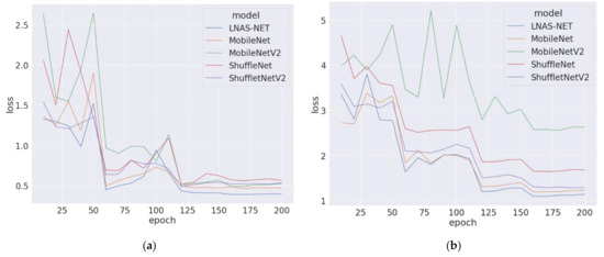
Figure 5.
(a) Loss value of training dataset food-11 in 200 epochs; (b) loss value of training dataset food-101 in 200 epochs.
As shown in Figure 5b, the gap of loss values between models are higher than in food-11. Food-101 is more difficult to be classified by the neural network. It has 101 labels, which are 9 times more than food-11. The proposed LNAS-NET is still able to maintain the lowest loss value throughout the training period. The loss value of MobileNet and ShuffetNetV2 are slightly worse than the proposed LNAS-NET. MobileNetV2 has an obvious larger gap than the rest of the models. Both figures demonstrate that our LNAS is able to generate a model that has better training performance than the hand-crafted models.
Now, we look into the accuracy of the validation set for every 50 epochs. Table 1 shows the validation accuracy on food-11 data. The higher accuracy value indicates the higher degree of closeness to true labels. In the 100th epoch, the accuracy of ShuffleNetV2 is 77.2%, which is 2.9% higher than LNAS-NET. However, the proposed LNAS-NET overtook the first place at 150th and 200th epochs in a long run. The final validation accuracy of the proposed LNAS-NET is 0.891, which is 3.7% higher than the second place. Compared to LNAS-NET, ShuffleNetV2 has a lower number of parameters that help reach the local minimum faster [35], but LNAS-NET proves to be more robust in a longer run.

Table 1.
Validation accuracy on food-11 dataset.
As shown in Table 2, the proposed LNAS-NET has the best validation accuracy for every checkpoint on food-101. It reached 32.8% in the first 50 epochs, which is 10% significantly higher than ShuffeNetV2. At the last epoch, the accuracy of LNAS is 70.7% on the validation set. The second place is ShuffleNetV2 with 66.3% and it is 4.4% lower than the proposed LNAS-NET. MobileNetV2 is not able to perform well on this complicated dataset. The validation accuracy is only 35.8% at the last epoch. In terms of training loss and validation accuracy, the proposed LNAS-NET outperformed the state-of-the-art models for both simple and complex food datasets.
Table 2.
Validation accuracy on food-101 dataset.
Table 3 shows the number of parameters and total time spent in 200 epochs of every model, along with the top-1 and top-5 accuracy on the test set. The top-1 and top-5 test accuracy for the proposed LNAS-NET are 89.1% and 99.2% respectively. It prevails over the second-best model, which is 1.7% and 0.2% higher than ShuffleNetV2. The efficiency of the proposed LNAS-NET is the key characteristic that sets it apart from other lightweight models. The training speed of the proposed LNAS-NET is 41.6% faster than ShuffleNetV2, equivalent to almost an hour in the actual time spent. Although ShuffleNetV2 has a fewer number of parameters, it did not lead to a faster training speed due to the mathematical complexity of the group convolution and the channel shuffle operation. On the other hand, MobileNet has a training speed closer with the proposed LNAS-NET, but its model is 86.12% larger than LNAS-NET. The smaller model often results in lower memory consumption during model interference.
Table 3.
Performance metric on test set for food-11.
Next, we look into the time spent and test accuracy for the food-101 dataset. As shown in Table 4, the proposed LNAS-NET achieved the highest top-1 and top-5 test accuracy with a notably faster training speed. Its training speed is 5.7 h faster than ShuffleNetV2. The efficiency of a model shows its importance when training with a bigger dataset. As regard of test accuracy, MobileNet has the second-best place after the proposed LNAS-NET. The top-1 and top-5 accuracy of the proposed LNAS-NET is 2.3% and 1% higher than MobileNet. The focus of this paper is to empower LNAS to design an ultra-lightweight CNN and yet maintain a satisfiable result. As a child model by LNAS, LNAS-NET shows an impressive performance in model efficiency and accuracy. It is able to remarkably improve the training speed and yet slightly improve the model accuracy.
Table 4.
Performance metric on test set for food-101.
In addition to the state-of-the-art models, the comparative analysis is made with the recent works to benchmark the performance of the proposed model on the food-101 dataset. The results were shown in Table 5. Linear SVM and fast χ2 kernel were proposed to provide real-time food recognition on mobile phones with an accuracy of 53.50% [36]. Martinel et al. suggested Extreme Learning Machine to slightly improve the performance of SVM [37]. Deep CNN was first tested by Bossard et al. on this dataset to achieve an accuracy rate of 56.40% [38]. Inspired by transfer learning, a pre-trained CNN obtained extra training data from ImageNet to fine-tune its feature extraction. This improves the accuracy rate to 70.41% [7]. Another notable work proposed by Pandey et al., to create an Ensemble CNN model by integrating AlexNet, GoogleNet, and ResNet into a multi-layered architecture, improved the accuracy rate by 1.71% [39]. With this additional analysis being done, this again proves that the proposed method manages to empower LNAS to design an ultra-lightweight CNN and yet maintain a satisfiable result. Despite being a lightweight model for efficient training and edge computing, LNAS-NET is still able to deliver a noteworthy accuracy rate when compared to other models.
Table 5.
Comparative analysis with recent works for food-101.
4. Conclusions
This paper proposed a novel Lightweight Neural Architecture Search (LNAS) to automate the process of building new CNN architecture for image-based food classification. LNAS deploys an RNN controller to execute a two-step approach to learn the controller parameters and shared parameters separately with the REINFORCE strategy. The proposed model by LNAS was tested and compared thoroughly with well-known lightweight models. The distinct features of this paper can be summarized as: (1) Authors propose a novel LNAS that involves a revolutionary search space with sophisticated convolution blocks and parameter sharing in DAG. Policy-based reinforcement learning allows the RNN controller to find the best child model and self-learning based on reward score. (2) As a child mode generated by LNAS, LNAS-NET comprises a state-of-the-art CNN architecture which is designed by LNAS with no human guidance during the training process. It has proven to deliver astonishing training speed and excellent accuracy on the food image classification. Furthermore, LNAS has no knowledge about food images when building LNAS-NET, since it was fed with general-purpose CIFAR-100 image data. The proposed LNAS-NET can be used in image classification for other domains as well, not only for food classification. Recently, researchers have shifted the interest from designing weighty models into mobile-friendly models that are able to run on edge devices. LNAS provides a good direction to incorporate some human-designed convolution blocks into the search space and let the controller decide the connection and parameters to design a child model from millions of possibilities.
For future work, it will be interesting to see if LNAS is able to design different types of neural networks such as CapsNet or Generative Adversarial Network. We can fine-tune the search space to include the necessary components of the targeted neural network. Furthermore, it is worth considering the alternative algorithm for the search strategy, i.e., Deep Q Network in further research. Finally, besides dietary assessment, it is also interesting to extend LNAS into other health-related applications such as designing the deep learning model to support a mobile-friendly digital sports coaching application.
Author Contributions
R.Z.T., X.Y.C. and K.W.K. contributed equally to this work. All authors have read and agreed to the published version of the manuscript.
Funding
This work is supported by the RUI (Individual) Grant by the Universiti Sains Malaysia (USM) under Grant No. 1001/PKOMP/8011136 for the project entitled “A New Adaptive Kernel-Distance-Based Control Chart by Machine Learning Techniques To Support Industry 4.0 Sustainable Smart Manufacturing”.
Institutional Review Board Statement
Not applicable.
Informed Consent Statement
Not applicable.
Data Availability Statement
Not applicable.
Conflicts of Interest
The authors declare no conflict of interest.
References
- Mohammadbeigi, A.; Asgarian, A.; Moshir, E.; Heidari, H.; Afrashteh, S.; Khazaei, S.; Ansari, H. Fast food consumption and overweight/obesity prevalence in students and its association with general and abdominal obesity. J. Prev. Med. Hyg. 2018, 59, E236–E240. [Google Scholar] [CrossRef] [PubMed]
- Ramirez, A.; Vadiveloo, M.; Greaney, M.; Risica, P.; Gans, K.; Mena, N.; Tovar, A. Dietary Contributors to Food Group Intake in Preschool Children Attending Family Childcare Homes. Curr. Dev. Nutr. 2020, 4, 268. [Google Scholar] [CrossRef]
- Fitt, E.; Cole, D.; Ziauddeen, N.; Pell, D.; Stickley, E.; Harvey, A.; Stephen, A.M. DINO (Diet In Nutrients Out)—An integrated dietary assessment system. Public Health Nutr. 2014, 18, 234–241. [Google Scholar] [CrossRef] [PubMed]
- Chen, Y.S.; Wong, J.E.; Ayob, A.F.; Othman, N.E.; Poh, B.K. Can Malaysian Young Adults Report Dietary Intake Using a Food Diary Mobile Application? A Pilot Study on Acceptability and Compliance. Nutrients 2017, 9, 62. [Google Scholar] [CrossRef]
- Khishe, M.; Caraffini, F.; Kuhn, S. Evolving Deep Learning Convolutional Neural Networks for Early COVID-19 Detection in Chest X-ray Images. Mathematics 2021, 9, 1002. [Google Scholar] [CrossRef]
- Tan, R.Z.; Chew, X.; Khaw, K.W. Quantized Deep Residual Convolutional Neural Network for Image-Based Dietary Assessment. IEEE Access 2020, 8, 111875–111888. [Google Scholar] [CrossRef]
- Yanai, K.; Kawano, Y. Food image recognition using deep convolutional network with pre-training and fine-tuning. In Proceedings of the 2015 IEEE International Conference on Multimedia & Expo Workshops (ICMEW), Turin, Italy, 29 June–3 July 2015; pp. 1–6. [Google Scholar]
- Michele, A.; Colin, V.; Santika, D.D. MobileNet Convolutional Neural Networks and Support Vector Machines for Palmprint Recognition. Procedia Comput. Sci. 2019, 157, 110–117. [Google Scholar] [CrossRef]
- Kc, K.; Yin, Z.; Wu, M.; Wu, Z. Depthwise separable convolution architectures for plant disease classification. Comput. Electron. Agric. 2019, 165, 104948. [Google Scholar] [CrossRef]
- Zhang, X.; Zhou, X.; Lin, M.; Sun, J. ShuffleNet: An Extremely Efficient Convolutional Neural Network for Mobile Devices. In Proceedings of the 2018 IEEE/CVF Conference on Computer Vision and Pattern Recognition, Salt Lake City, UT, USA, 18–23 June 2018; pp. 6848–6856. [Google Scholar]
- Freeman, I.; Roese-Koerner, L.; Kummert, A. Effnet: An Efficient Structure for Convolutional Neural Networks. In Proceedings of the 2018 25th IEEE International Conference on Image Processing (ICIP), Athens, Greece, 7–10 October 2018; pp. 6–10. [Google Scholar]
- Elsken, T.; Metzen, J.H.; Hutter, F. Neural Architecture Search: A Survey. arXiv 2019, arXiv:1808.05377. [Google Scholar]
- He, X.; Zhao, K.; Chu, X. AutoML: A survey of the state-of-the-art. Knowl. Based Syst. 2021, 212, 106622. [Google Scholar] [CrossRef]
- Asadulaev, A.; Kuznetsov, I.; Stein, G.; Filchenkov, A. Exploring and Exploiting Conditioning of Reinforcement Learning Agents. IEEE Access 2020, 8, 211951–211960. [Google Scholar] [CrossRef]
- Ben-Nun, T.; Hoefler, T. Demystifying Parallel and Distributed Deep Learning: An In-Depth Concurrency Analysis. ACM Comput. Surv. 2019, 52, 65. [Google Scholar] [CrossRef]
- Hanif, M.S.; Bilal, M. Competitive residual neural network for image classification. ICT Express 2020, 6, 28–37. [Google Scholar] [CrossRef]
- Wang, J.; Li, S.; An, Z.; Jiang, X.; Qian, W.; Ji, S. Batch-normalized deep neural networks for achieving fast intelligent fault diagnosis of machines. Neurocomputing 2019, 329, 53–65. [Google Scholar] [CrossRef]
- Wu, S.; Li, G.; Deng, L.; Liu, L.; Wu, D.; Xie, Y.; Shi, L. L1-Norm Batch Normalization for Efficient Training of Deep Neural Networks. IEEE Trans. Neural Netw. Learn. Syst. 2018, 30, 2043–2051. [Google Scholar] [CrossRef]
- Guo, K.; Sui, L.; Qiu, J.; Yu, J.; Wang, J.; Yao, S.; Han, S.; Wang, Y.; Yang, H. Angel-Eye: A Complete Design Flow for Mapping CNN onto Embedded FPGA. IEEE Trans. Comput. Aided Des. Integr. Circuits Syst. 2018, 37, 35–47. [Google Scholar] [CrossRef]
- Zhang, X.; Sun, Y.; Wang, Y.; Li, Z.; Li, N.; Su, J. A novel effective and efficient capsule network via bottleneck residual block and automated gradual pruning. Comput. Electr. Eng. 2019, 80, 106481. [Google Scholar] [CrossRef]
- Lee, D. Comparison of Reinforcement Learning Activation Functions to Improve the Performance of the Racing Game Learning Agent. J. Inf. Process. Syst. 2020, 16, 1074–1082. [Google Scholar] [CrossRef]
- Li, Y.; Zhang, D.; Lee, D.-J. IIRNet: A lightweight deep neural network using intensely inverted residuals for image recognition. Image Vis. Comput. 2019, 92, 103819. [Google Scholar] [CrossRef]
- Horiguchi, S.; Ikami, D.; Aizawa, K. Significance of Softmax-based Features in Comparison to Distance Metric Learning-based Features. IEEE Trans. Pattern Anal. Mach. Intell. 2019, 42, 1279–1285. [Google Scholar] [CrossRef]
- Bhagat, S.; Banerjee, H.; Tse, Z.T.H.; Ren, H. Deep Reinforcement Learning for Soft, Flexible Robots: Brief Review with Impending Challenges. Robotics 2019, 8, 4. [Google Scholar] [CrossRef]
- Weng, J.; Jiang, X.; Zheng, W.-L.; Yuan, J. Early Action Recognition with Category Exclusion Using Policy-Based Reinforcement Learning. IEEE Trans. Circuits Syst. Video Technol. 2020, 30, 4626–4638. [Google Scholar] [CrossRef]
- Bohme, M.; Pham, V.-T.; Roychoudhury, A. Coverage-Based Greybox Fuzzing as Markov Chain. IEEE Trans. Softw. Eng. 2019, 45, 489–506. [Google Scholar] [CrossRef]
- Chen, M.; Beutel, A.; Covington, P.; Jain, S.; Belletti, F.; Chi, E. Top-K Off-Policy Correction for a REINFORCE Recommender System. arXiv 2020, arXiv:1812.02353. [Google Scholar]
- Chaudhari, P.; Soatto, S. Stochastic Gradient Descent Performs Variational Inference, Converges to Limit Cycles for Deep Networks. arXiv 2018, arXiv:1710.11029. [Google Scholar]
- Park, J.; Yi, D.; Ji, S. A Novel Learning Rate Schedule in Optimization for Neural Networks and It’s Convergence. Symmetry 2020, 12, 660. [Google Scholar] [CrossRef]
- Oyedotun, O.K.; Shabayek, A.E.R.; Aouada, D.; Ottersten, B. Improved Highway Network Block for Training Very Deep Neural Networks. IEEE Access 2020, 8, 176758–176773. [Google Scholar] [CrossRef]
- Yunus, R.; Arif, O.; Afzal, H.; Amjad, M.F.; Abbas, H.; Bokhari, H.N.; Haider, S.T.; Zafar, N.; Nawaz, R. A Framework to Estimate the Nutritional Value of Food in Real Time Using Deep Learning Techniques. IEEE Access 2019, 7, 2643–2652. [Google Scholar] [CrossRef]
- Krizhevsky, A.; Sutskever, I.; Hinton, G.E. ImageNet Classification with Deep Convolutional Neural Networks. Commun. ACM 2017, 60, 84–90. [Google Scholar] [CrossRef]
- Kutzner, C.; Páll, S.; Fechner, M.; Esztermann, A.; de Groot, B.L.; Grubmüller, H. More bang for your buck: Improved use of GPU nodes for GROMACS 2018. J. Comput. Chem. 2019, 40, 2418–2431. [Google Scholar] [CrossRef]
- Hu, K.; Zhang, Z.; Niu, X.; Zhang, Y.; Cao, C.; Xiao, F.; Gao, X. Retinal vessel segmentation of color fundus images using multiscale convolutional neural network with an improved cross-entropy loss function. Neurocomputing 2018, 309, 179–191. [Google Scholar] [CrossRef]
- Ma, N.; Zhang, X.; Zheng, H.-T.; Sun, J. ShuffleNet V2: Practical Guidelines for Efficient CNN Architecture Design. arXiv 2018, arXiv:1807.11164. [Google Scholar]
- Kawano, Y.; Yanai, K. Real-Time Mobile Food Recognition System. In Proceedings of the 2013 IEEE Conference on Computer Vision and Pattern Recognition Workshops, Portland, OR, USA, 23–28 June 2013; pp. 1–7. [Google Scholar]
- Martinel, N.; Piciarelli, C.; Micheloni, C. A supervised extreme learning committee for food recognition. Comput. Vis. Image Underst. 2016, 148, 67–86. [Google Scholar] [CrossRef]
- Bossard, L.; Guillaumin, M.; Van Gool, L. Food-101—Mining Discriminative Components with Random Forests. In Computer Vision—ECCV 2014; Fleet, D., Pajdla, T., Schiele, B., Tuytelaars, T., Eds.; Lecture Notes in Computer Science; Springer International Publishing: Cham, Switzerland, 2014; Volume 8694, pp. 446–461. ISBN 978-3-319-10598-7. [Google Scholar]
- Pandey, P.; Deepthi, A.; Mandal, B.; Puhan, N.B. FoodNet: Recognizing Foods Using Ensemble of Deep Networks. IEEE Signal Process. Lett. 2017, 24, 1758–1762. [Google Scholar] [CrossRef]


Publisher’s Note: MDPI stays neutral with regard to jurisdictional claims in published maps and institutional affiliations. |
© 2021 by the authors. Licensee MDPI, Basel, Switzerland. This article is an open access article distributed under the terms and conditions of the Creative Commons Attribution (CC BY) license (https://creativecommons.org/licenses/by/4.0/).