A Survey on Domination in Vague Graphs with Application in Transferring Cancer Patients between Countries

Abstract

Many problems of practical interest can be modeled and solved by using fuzzy graph (FG) algorithms. In general, fuzzy graph theory has a wide range of application in various fields. Since indeterminate information is an essential real-life problem and is often uncertain, modeling these problems based on FG is highly demanding for an expert. A vague graph (VG) can manage the uncertainty relevant to the inconsistent and indeterminate information of all real-world problems in which fuzzy graphs may not succeed in bringing about satisfactory results. Domination in FGs theory is one of the most widely used concepts in various sciences, including psychology, computer sciences, nervous systems, artificial intelligence, decision-making theory, etc. Many research studies today are trying to find other applications for domination in their field of interest. Hence, in this paper, we introduce different kinds of domination sets, such as the edge dominating set (EDS), the total edge dominating set (TEDS), the global dominating set (GDS), and the restrained dominating set (RDS), in product vague graphs (PVGs) and try to represent the properties of each by giving some examples. The relation between independent edge sets (IESs) and edge covering sets (ECSs) are established. Moreover, we derive the necessary and sufficient conditions for an edge dominating set to be minimal and show when a dominance set can be a global dominance set. Finally, we try to explain the relationship between a restrained dominating set and a restrained independent set with an example. Today, we see that there are still diseases that can only be treated in certain countries because they require a long treatment period with special medical devices. One of these diseases is leukemia, which severely affects the immune system and the body’s defenses, making it impossible for the patient to continue living a normal life. Therefore, in this paper, using a dominating set, we try to categorize countries that are in a more favorable position in terms of medical facilities, so that we can transfer the patients to a suitable hospital in the countries better suited in terms of both cost and distance.

1. Introduction

Fuzzy set theory and the related fuzzy logic were proposed by Zadeh [1] for dealing with and solving various problems in which variables, parameters, and relations are only imprecisely known, and hence, for which approximate reasoning schemes should be used. Such a situation is common in the case of virtually all nontrivial and, in particular, human-centered phenomena, processes, and systems that prevail in reality, and it is difficult to use conventional mathematics, based on binary logic, for their adequate characterization. Fuzzy set theory has been developed in many directions and has evoked great interest among mathematicians and computer scientists working in different fields of mathematics. Rosenfeld [2] used the concept of a fuzzy subset of a set to introduce the notion of a fuzzy subgroup of a group. Rosenfeld’s paper spearheaded the development of fuzzy abstract algebra. Zadeh [3] introduced the notion of interval-valued fuzzy sets as an extension of fuzzy sets, in which the values of the membership degrees are intervals of numbers instead of the numbers themselves. Interval-valued fuzzy sets provide a more adequate description of uncertainty than traditional fuzzy sets. It is therefore important to use interval-valued fuzzy sets in applications such as fuzzy control. One of the most computationally intensive parts of fuzzy control is defuzzification [4]. Since interval-valued fuzzy sets are widely studied and used, we briefly describe the work of Gorzalczany on approximate reasoning [5,6] and Roy and Biswas on medical diagnosis [7]. The notion of vague set theory, a generalization of Zadeh’s fuzzy set theory, was introduced by Gau and Buehrer [8] in 1993.

A graph is a very general and powerful formal and algorithmic tool for representation modeling, analyses, and solutions of a multitude of complex real-world problems. An immediate result of the popularity of fuzzy set theory was graph theory fuzzification, which was instigated by Rosenfeld [9], who proposed the concept of FG and many related concepts and properties, such as paths, cycles, and connectedness. Basically, an FG is a weighted graph in which the weights are in the range of $[0,1]$ and are defined over a fuzzy set of vertices. FG models are expedient mathematical tools for dealing with different domains of combinatorial problems in algebra, topology, optimization, the computer sciences, and the social sciences. FG models outperform graph models due to the natural existence of vagueness and ambiguity. Gau and Buehrer [8] described VS theory by providing a definition of the notion of VS by changing an element value in a set with a [0;1] subinterval. A VS is highly effective for explaining the existence of the false membership degree. Furthermore, Kauffmann [10] introduced FGs based on Zadeh’s fuzzy relation [3], and Gupta et al. [11] used fuzzy set theory in medical sciences. Moreover, Akram et al. [12,13,14,15,16,17,18,19,20,21] developed several concepts and results on vague graphs, and Mordeson et al. [22,23,24] studied some results in FGs. Pal et al. [25,26,27] represented the fuzzy competition graph and presented some remarks on bipolar fuzzy graphs, and Borzooei et al. [28,29,30,31,32] analyzed several concepts of VGs. In addition, Shao et al. [33] defined new results in FGs and intuitionistic fuzzy graphs, Szmidt and Kacprzyk [34] described intuitionistic fuzzy sets in some medical applications, Davvaz and Hassani Sadrabadi [35] studied an application of an intuitionistic fuzzy set in medicine, Dutta et al. [36] introduced fuzzy decision making in medical diagnosis using an advanced distance measure on intuitionistic fuzzy sets, and, finally, Ramakrishna [37] proposed the concepts of VG and examined the properties. Kosari et al. [38] defined vague graph structure and studied its properties.

A PVG is referred to as a generalized structure of an FG that delivers more exactness, adaptability, and compatibility to a system when matched with systems running on FGs. Furthermore, a PVG is able to concentrate on determining the uncertainty coupled with the inconsistent and indeterminate information of any real-world problems, whereas FGs may not lead to adequate results.

Domination in PVGs theory is one of the most widely used concepts in various sciences, including psychology, computer science, nervous systems, artificial intelligence, decision-making theory, and various combinations. Many authors today are trying to find other uses for domination in their fields of interest. The dominance of FGs has been stated by various researchers, but, as a result of PVGs being broader and more widely used than FGs, today, it is used in many branches of engineering and medical sciences. Similarly, it has many applications for the formulation and solution of a multitude of problems in various areas of science and technology, such as computer networks, artificial intelligence, combinatorial analyses, etc. Therefore, considering its importance, we attempted to study different types of domination of PVGs and examine their properties by giving examples. Furthermore, we present an application of domination in PVGs in the field of medicine. Ore [39] pioneered the application of the expression “domination” for undirected graphs. Somasundaram [40] defined domination and independent domination in FGs. Shubatah et al. [41] studied edge domination in intuitionistic fuzzy graphs. Mahioub and Shubatah [42,43] investigated domination in product fuzzy graphs. Gani and Chandrasekaran [44,45] introduced notions of fuzzy DS and independent DS utilizing strong arcs. The domination concept in intuitionistic fuzzy graphs was examined by Parvathi and Thamizhendhi [46]. Manjusha and Sunitha [47,48] studied coverings, matchings, and paired domination in fuzzy graphs using strong arcs. Gang et al. [49] investigated total efficient domination in fuzzy graphs. Karunambigai et al. [50] introduced domination in bipolar fuzzy graphs. Cockayne [51] and Hedetniemi [52] described the independent and irredundance domination number in graphs.

Domination in PVGs is so important that it can play a vital role in decision-making theory, which concerns finding the best possible state in a test or experiment. Although some DSs in FGs have been proposed by a number of authors, the breadth of the subject and its various applications in engineering and medicine, and the limitations of past definitions, prompted us to introduce new types of DSs on the PVG. In fact, the limitations of the old definitions in FGs forced us to come up with new definitions in PVGs. Hence, in this study, we represent different kinds of DSs, such as EDS, TEDS, GDS, and RDS, in PVGs and also try to described the properties of each by giving some examples. The relationship between IESs and ECSs are established. A comparative study between “EDS and Minimal-EDS”, and “IES and Maximal-IES” was conducted. Some remarkable properties associated with these new DSs were investigated, and the necessary and sufficient condition for a DS to be a GDS was stated. Finally, we defined RIS and RDS and examined the relationships between them in a theorem. Today, many cancer patients pass away due to the lack of the necessary medical equipment in their country. Therefore, it is indispensable to identify the countries that have the necessary conditions to treat such patients. Hence, in this paper, with the help of DS, we attempt to identify countries that are in a more favorable position in terms of medical facilities, so that we can transfer the patients to a suitable hospital in these countries, which are better suited in terms of both cost and distance.

2. Preliminaries

In the following, some basic concepts on VGs are reviewed in order to facilitate the next section.

A graph $G^{*}=(V,E)$ is a mathematical structure containing of a set of nodes V and a set of edges E, so that every edge is an unordered pair of distinct nodes. An FG has the form of $\zeta =(\gamma ,\nu )$, where $\gamma :V\to [0,1]$ and $\nu :V\times V\to [0,1]$ is defined as $\nu \left(mn\right)\le \gamma \left(m\right)\wedge \gamma \left(n\right)$, $\forall m,n\in V$, and $\nu$ is a symmetric fuzzy relation on $\gamma$, and ∧ denotes the minimum.

Definition 1.

([8]) A VS A is a pair $(t_A,f_A)$ on set V, where $t_A$ and $f_A$ are used as real-valued functions, which can be defined on $V\to [0,1]$, so that $t_A\left(m\right)+f_A\left(m\right)\le 1$, $\forall m\in V$.

$G^{*}$ is a crisp graph $(V,E)$ and $\zeta$ a VG $(A,B)$ throughout this paper.

Definition 2.

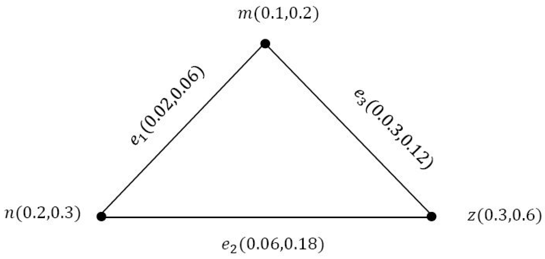
([37]) A pair $\zeta =(A,B)$ is called a VG on a crisp graph $G^{*}$, so that $A=(t_A,f_A)$ is a VS on V and $B=(t_B,f_B)$ is a VS on $E\subseteq V\times V$, so that $t_B\left(mn\right)\le min(t_A\left(m\right),t_A\left(n\right))$ and $f_B\left(mn\right)\ge max(f_A\left(m\right),f_A\left(n\right))$, $\forall mn\in E$.

Example 1.

Consider a VG ζ as in Figure 1, such that $V=\{m,n,z\}$, $E=\{mn,nz,mz\}$.

By routine computations, it is easy to show that ζ is a VG.

Definition 3.

([17]) Let $\zeta =(A,B)$ be a VG.

$\left(i\right)$ The cardinality of ζ is defined as:

$$\left|\zeta \right|=|\sum _{m_i\in V}{\displaystyle \frac{1+t_A\left(m_i\right)-f_A\left(m_i\right)}{2}}+\sum _{m_i{n}_i\in E}{\displaystyle \frac{1+t_B\left(m_i{n}_i\right)-f_B\left(m_i{n}_i\right)}{2}}|;$$

$\left(ii\right)$ The vertex cardinality of ζ is defined as $\left|V\right|={\sum }_{m_i\in V}{\displaystyle \frac{1+t_A\left(m_i\right)-f_A\left(m_i\right)}{2}}$, $\forall m_i\in V$, is called the order of a VG ζ, and is denoted by $p\left(\zeta \right)$;

$\left(iii\right)$ The edge cardinality of ζ is defined as $\left|E\right|={\sum }_{m_i{n}_i\in E}{\displaystyle \frac{1+t_B\left(m_i{n}_i\right)-f_B\left(m_i{n}_i\right)}{2}}$, $\forall m_i{n}_i\in E$, is called the size of a VG ζ, and is denoted by $q\left(\zeta \right)$.

Example 2.

In Example 1, it is easy to show that

$$\begin{array}{ccc}& & \left|V\right|=0.45+0.4+0.35=1.2,\hfill \\ & & \left|E\right|=0.3+0.25+0.35=0.9.\hfill \end{array}$$

Definition 4.

([46]) Let $\zeta =(A,B)$ be a VG. If $m_i,m_j\in V$, then the t-strength of connectedness between $m_i$ and $m_j$ is defined as $t_B^{\infty }(m_i,m_j)=sup\left\{t_B^k(m_i,m_j)\right|k=1,2,\cdots ,n\}$ and the f-strength of connectedness between $m_i$ and $m_j$ is defined as $f_B^{\infty }(m_i,m_j)=inf\left\{f_B^k(m_i,m_j)\right|k=1,2,\cdots ,n\}$. Furthermore, we have

$$\begin{array}{ccc}& & t_B^k\left(mn\right)=sup\{t_B(m,n_1)\wedge t_B(n_1,n_2)\wedge t_B(n_2,n_3)\wedge \cdots \wedge t_B(n_{k-1},n)|\hfill \\ & & (m,n_1,n_2,\cdots ,n_{k-1},n)\in V\}\hfill \end{array}$$

and

$$\begin{array}{ccc}& & f_B^k\left(mn\right)=inf\{f_B(m,n_1)\vee f_B(n_1,n_2)\vee f_B(n_2,n_3)\vee \cdots \vee f_B(n_{k-1},n)|\hfill \\ & & (m,n_1,n_2,\cdots ,n_{k-1},n)\in V\}.\hfill \end{array}$$

Example 3.

In Example 1, the t-strength of connectedness and the f-strength of connectedness for edge $mz$ are as follows:

$$t_B^{\infty }\left(mz\right)=0.1,f_B^{\infty }\left(mz\right)=0.4.$$

Definition 5.

([46]) An edge $mn$ in a VG $\zeta =(A,B)$ is called the strong edge if $t_B\left(mn\right)\ge {\left(t_B\right)}^{\infty }\left(mn\right)$ and $f_B\left(mn\right)\le {\left(f_B\right)}^{\infty }\left(mn\right)$.

Example 4.

Consider the VG ζ as in Figure 2.

Clearly, $e_1$ and $e_2$ are strong edges.

Definition 6.

([46]) The two vertices $m_i$ and $m_j$ are said to be neighbors in a VG ζ if either one of the following conditions holds:

(i)

$t_B\left(m_i{m}_j\right)>0,f_B\left(m_i{m}_j\right)>0$;

(ii)

$\left(ii\right)$$t_B\left(m_i{m}_j\right)=0,f_B\left(m_i{m}_j\right)>0$;

(iii)

$\left(iii\right)$$t_B\left(m_i{m}_j\right)>0,f_B\left(m_i{m}_j\right)=0,m_i,m_j\in V$.

The two vertices $m_i$ and $m_j$ are said to be strong neighbors if $t_B\left(m_i{m}_j\right)=min\{t_A\left(m_i\right),t_A\left(m_j\right)\}$ and $f_B\left(m_i{m}_j\right)=max\{f_A\left(m_i\right),f_A\left(m_j\right)\}$.

Definition 7.

([18]) A VG $\zeta =(A,B)$ is called complete if $t_B\left(m_i{m}_j\right)=min\{t_A\left(m_i\right),t_A\left(m_j\right)\}$ and $f_B\left(m_i{m}_j\right)=max\{f_A\left(m_i\right),f_A\left(m_j\right)\}$, $\forall m_i,m_j\in V$.

VG ζ is called strong if $t_B\left(m_i{m}_j\right)=min\{t_A\left(m_i\right),t_A\left(m_j\right)\}$ and $f_B\left(m_i{m}_j\right)=max\{f_A\left(m_i\right),f_A\left(m_j\right)\}$, $\forall m_i{m}_j\in E$.

Definition 8.

([29]) Let $\zeta =(A,B)$ be a VG. Suppose that $m,n\in V$, we say that m dominates n in ζ if there exists a strong edge between them.

A subset S of V is called a DS in $\zeta$ if for each $m\in V-S$, ∃$n\in S$, so that m dominated n. A DS S of a VG $\zeta$ is referred to as a minimal DS if no proper subset of S is a DS.

Example 5.

Consider the VG ζ as in Figure 3.

It is easy to show that $\{m,n,z\}$ and $\{n,z,w\}$ are DSs.

Definition 9.

([18]) The complement of a VG $\zeta =(A,B)$ is a pair $\overline{G}=(\overline{A},\overline{B})$, where $\overline{A}=A$ and $\overline{B}=(\overline{t_B},\overline{f_B})$ are defined as

$$\begin{array}{ccc}& & \overline{t_B}\left(mn\right)=t_A\left(m\right)\wedge t_A\left(n\right)-t_B\left(mn\right),and\hfill \\ & & \overline{f_B}\left(mn\right)=f_B\left(mn\right)-f_A\left(m\right)\vee f_A\left(n\right),\forall mn\in E.\hfill \end{array}$$

Definition 10.

([32]) Let $\zeta =(A,B)$ be a VG. If $t_B\left(mn\right)\le t_A\left(m\right)\times t_A\left(n\right)$ and $f_B\left(mn\right)\ge f_A\left(m\right)\times f_A\left(n\right)$, $\forall m,n\in V$, then the VG ζ is called PVG. Note that a PVG ζ is not necessarily a VG. A PVG ζ is called a complete PVG if $t_B\left(mn\right)=t_A\left(m\right)\times t_A\left(n\right)$ and $f_B\left(mn\right)=f_A\left(m\right)\times f_A\left(n\right)$, $\forall m,n\in V$.

The complement of PVG $\zeta =(A,B)$ is $\overline{\zeta }=(\overline{A},\overline{B})$, where, $\overline{A}=A=(t_A,f_A)$ and $\overline{B}=(\overline{t_B},\overline{f_B})$, so that $\overline{t_B}\left(mn\right)=t_A\left(m\right)\times t_A\left(n\right)-t_B\left(mn\right)$ and $\overline{f_B}\left(mn\right)=f_B\left(mn\right)-f_A\left(m\right)\times f_A\left(n\right)$.

Example 6.

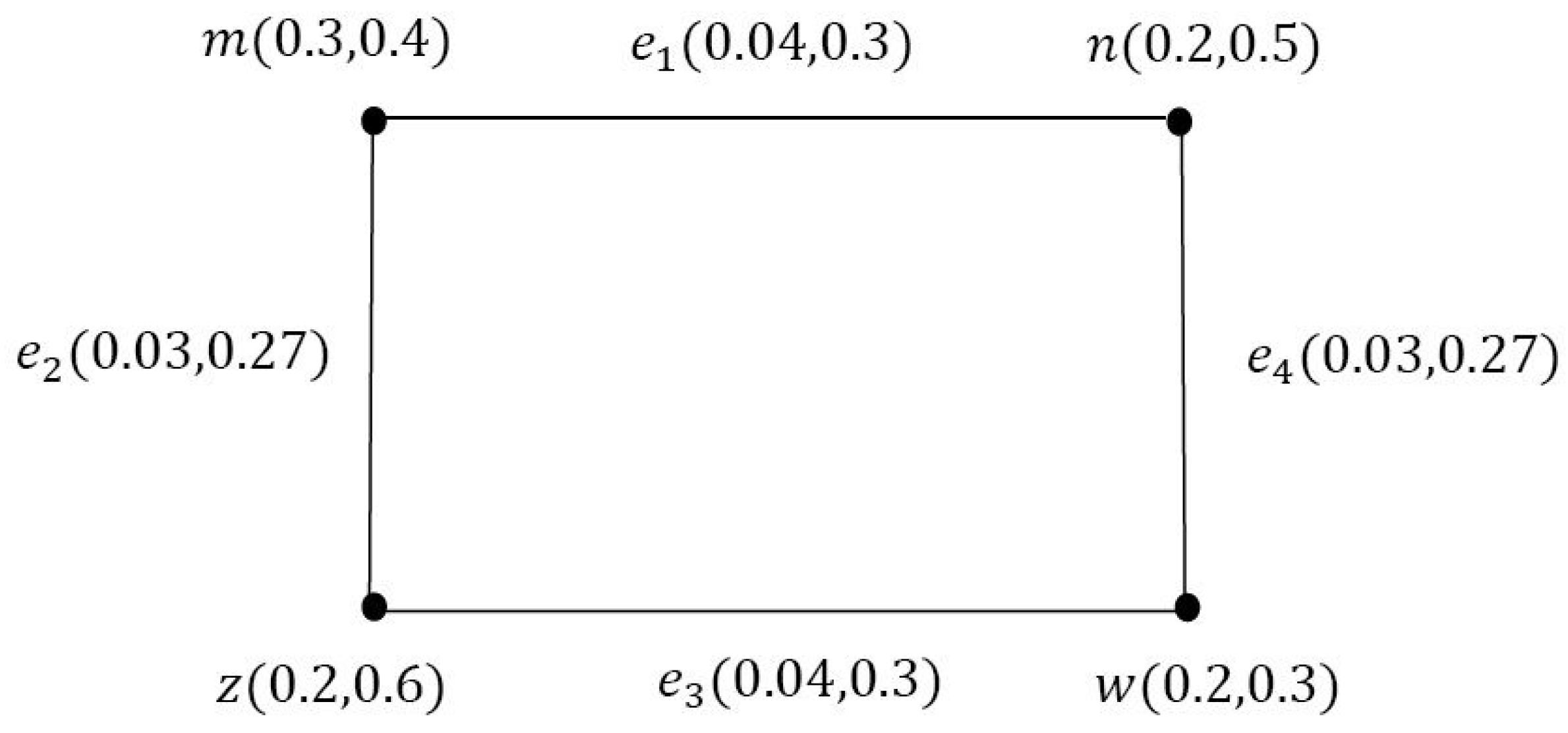
Consider the PVG ζ as in Figure 4.

Obviously, ζ is a PVG since it has the condition of Definition 10.

Definition 11.

([43]) An edge $mn$ in a PVG ζ is called an effective edge if $t_B\left(mn\right)=t_A\left(m\right)\times t_A\left(n\right)$ and $f_B\left(mn\right)=f_A\left(m\right)\times f_A\left(n\right)$.

Example 7.

In Example 6, $mn$ is an effective edge.

$$\begin{array}{ccc}& & 0.06=t_B\left(mn\right)=0.2\times 0.3,\hfill \\ & & 0.12=f_B\left(mn\right)=0.3\times 0.4.\hfill \end{array}$$

Definition 12.

([43]) If ζ be a PVG, then the vertex cardinality of $S\subseteq V$ is defined as

$$\left|S\right|=\left|\sum _{m\in S}{\displaystyle \frac{1+t_A\left(m\right)-f_A\left(m\right)}{2}}\right|.$$

Definition 13.

([43]) Let $\zeta =(A,B)$ be a PVG, then the edge cardinality of $K\subseteq E$ is defined as

$$\left|K\right|=\left|\sum _{mn\in K}{\displaystyle \frac{1+t_B\left(mn\right)-f_B\left(mn\right)}{2}}\right|.$$

Definition 14.

([43]) Two edges $mn$ and $zw$ in a PVG ζ are said to be adjacent if they are neighbors. Furthermore, they are independent if they are not adjacent.

Definition 15.

([29]) Let $\zeta =(A,B)$ be a PVG. A vertex subset S of $V\left(\zeta \right)$ is called a DS of ζ if for every node $m\in V-S$, ∃ a node $n\in S$, so that

$$t_B\left(mn\right)=t_A\left(m\right)\times t_A\left(n\right)and{f}_B\left(mn\right)=f_A\left(m\right)\times f_A\left(n\right).$$

Example 8.

Consider the PVG ζ as in Figure 5.

It is easy to show that $S=\{n,z\}$ is a DS.

Definition 16.

([43]) Let $\zeta =(A,B)$ be a PVG. Then, the degree of a node m is defined as $deg\left(m\right)=({deg}^t\left(m\right),{deg}^f\left(m\right))=(M_1,M_2)$, where $M_1={\sum }_{m\ne n}{t}_B\left(mn\right)$ and $M_2={\sum }_{m\ne n}{f}_B\left(mn\right)$, for $mn\in E$.

A PVG ζ is said to be a $(M_1,M_2)$-regular if $deg\left(m_i\right)=(M_1,M_2)$, $\forall m_i\in V$.

Example 9.

In Example 8, we have

$$deg\left(m\right)=(0.05,0.18)anddeg\left(z\right)=(0.09,0.3).$$

Definition 17.

([43]) Two nodes in a PVG ζ are said to be independent if there is no strong arc between them. A subset S of V is said to be an independent set if every two nodes of S are independent.

All the basic notations are shown in

Table 1. Some basic notations.

Notation	Meaning
FG	Fuzzy Graph
VS	Vague Set
VG	Vague Graph
DS	Dominating Set
EDS	Edge Dominating Set
TEDS	Total Edge Dominating Set
GDS	Global Dominating Set
EIS	Edge Independent Set
RDS	Restrained Dominating Set
IES	Independent Edge Set
GDN	Global Dominating Number
EIN	Edge Independent Number
ECS	Edge Covering Set
ECN	Edge Covering Number
EDN	Edge Dominating Number
TEDN	Total Edge Dominating Number
PVG	Product Vague Graph
RIS	Restrained Independent Set

.

3. Edge Domination in PVGs

Definition 18.

An edge subset K of E in a PVG ζ is said to be independent (IES) if $t_B\left(mn\right)<t_A\left(m\right)\times t_A\left(n\right)$ and $f_B\left(mn\right)>f_A\left(m\right)\times f_A\left(n\right)$, $\forall m,n\in K$. The maximum cardinality among all maximal IES in ζ is called the EIN and it is denoted by ${\beta }_1\left(\zeta \right)$ or simply ${\beta }_1$.

Example 10.

Consider the PVG ζ as in Figure 6.

Here, $\{e_1,e_2\}$, $\{e_1,e_4\}$, $\{e_2,e_4\}$, and $\{e_1,e_2,e_4\}$ are IESs of ζ and ${\beta }_1\left(\zeta \right)=0.84$.

Definition 19.

An edge $mn$ and a vertex z in a PVG ζ are said to cover each other if they are incident.

Definition 20.

An edge subset K of E in a PVG ζ, which covers all nodes in ζ, is called an ECS of ζ. The minimum cardinality among all ECS is called the ECN of ζ and it is denoted by ${\alpha }_1\left(\zeta \right)$ or simply ${\alpha }_1$.

Example 11.

Consider the PVG ζ in Figure 7.

Here, $\{e_1,e_3\}$ and $\{e_2,e_4\}$ are ECSs and ${\alpha }_1\left(\zeta \right)=0.5$.

Theorem 1.

An edge subset $K\subseteq E$ in a PVG ζ is an independent set in ζ if $E-K$ is an ECS of ζ.

Proof. 

By definition, K is an independent set if and only if no two edges of K are adjacent, if and only if every edge of K is incident with at least one vertex of $E-K$, and if and only if $E-K$ is an ECS of $\zeta$. □

Example 12.

Consider the PVG ζ as in Figure 7. It is easy to show that $K=\{e_1,e_3\}$ is an independent set and $E-K=\{e_2,e_4\}$ is an ECS.

Definition 21.

An edge e of a PVG ζ is said to be an isolated edge if no effective edges are incident with the vertices of e. Hence, an isolated edge does not dominate any other edge in ζ.

Example 13.

In Example 11, it is easy to show that the edges $mn$ and $nw$ are isolated edges.

Definition 22.

Let e be any edge in a PVG ζ.

Then, $N\left(e\right)=\{m\in E:misaneffectiveedgeincidentwiththenodesofe\}$ and is called the open edge neighborhood set of e. $N\left[e\right]=N\left(e\right)\cup \left\{e\right\}$ is called the closed neighborhood set of e.

Definition 23.

Let e be any edge in a PVG ζ. Then, $d_N\left(e\right)={\sum }_{m\in N\left(e\right)}\left|m\right|$ is called the edge neighborhood degree of e. The minimum edge neighborhood degree of a PVG ζ is ${\delta }_N^{\prime }\left(\zeta \right)=min\left\{d_N\left(e\right)\right|e\in E\}$. The maximum edge neighborhood degree of a PVG ζ is ${\mathsf{\Delta }}_N^{\prime }\left(\zeta \right)=max\left\{d_N\left(e\right)\right|e\in E\}$.

Example 14.

Consider the PVG ζ as in Figure 8.

It is clear that $N\left(e_1\right)=\{e_2,e_5\}$ and $d_N\left(e_1\right)=0.91$.

Theorem 2.

For any PVG $\zeta =(A,B)$ without isolated edges, ${\alpha }_1\left(\zeta \right)+{\beta }_1\left(\zeta \right)=q$.

Proof. 

Let K be an EIS in $\zeta$ and S be an ECS in $\zeta$ so that $\left|K\right|={\beta }_1\left(\zeta \right)$ and $\left|S\right|={\alpha }_1\left(\zeta \right)$. Then, by Theorem 1, $E-K$ is an ECS of $\zeta$. Therefore, $\left|S\right|\le |E-K|$ and ${\alpha }_1\left(\zeta \right)\le q-{\beta }_1\left(\zeta \right)$ or

$${\alpha }_1\left(\zeta \right)+{\beta }_1\left(\zeta \right)\le q.$$

(1)

Furthermore, by Theorem 1, $E-S$ is an EIS in $\zeta$, so $\left|K\right|\ge |E-S|$. Therefore, ${\beta }_1\left(\zeta \right)\ge q-{\alpha }_1\left(\zeta \right)$ or

$${\alpha }_1\left(\zeta \right)+{\beta }_1\left(\zeta \right)\ge q.$$

(2)

From (1) and (2), we obtain ${\alpha }_1\left(\zeta \right)+{\beta }_1\left(\zeta \right)=q$. □

Example 15.

In Example 11, we have

$${\alpha }_1\left(\zeta \right)=0.5,{\beta }_1\left(\zeta \right)=0.52,andq=1.02.$$

Therefore, Theorem 2 holds.

Definition 24.

Let $\zeta =(A,B)$ be a PVG and $e_i$ and $e_j$ be two adjacent edges of ζ. We say that $e_i$ dominates $e_j$ if $e_i$ is an effective edge. An edge subset K of E in a PVG ζ is called an EDS if, for each edge $e_i\in E-K$, ∃ an effective edge $e_j\in K$ so that $e_j$ dominates $e_i$. An EDS K of a PVG ζ is said to be a minimal EDS if for each edge $e\in K$, $K-\left\{e\right\}$ is not an EDS. The minimum cardinality between all minimal EDSs is called an EDN of ζ and is described by ${\gamma }^{\prime }\left(\zeta \right)$ or simply ${\gamma }^{\prime }$. An EDS K of a PVG ζ is said to be independent if $t_B\left(mn\right)<t_A\left(m\right)\times t_A\left(n\right)$ and $f_B\left(mn\right)>f_A\left(m\right)\times f_A\left(n\right)$, $\forall (m,n)\in K$.

Example 16.

Consider the VG ζ as in Figure 9.

In this example, $\{e_1,e_2\}$, $\{e_2,e_4\}$, $\{e_3,e_4\}$, and $\{e_1,e_3\}$ are EDSs and ${\gamma }^{\prime }\left(\zeta \right)=0.84$.

Theorem 3.

An EDS K in PVG ζ is a minimal EDS if and only if for each edge $e\in K$, one of the following two conditions holds:

(i)

$N\left(e\right)\cap K=\varnothing$;

(ii)

∃ an edge $e\in E-K$ so that $N\left(e\right)\cap K=\left\{e\right\}$ and e is an effective edge.

Proof. 

Let K be a minimal EDS and $e\in K$. Then, $K_e=K-\left\{e\right\}$ is not an EDS and hence ∃$t\in E-K_e$, so that t is not dominated by any element of $K_e$. If $t=e$, we obtain $\left(i\right)$ and if $t\ne e$, we obtain $\left(ii\right)$. Conversely, assume that K is an EDS, and for each edge $e\in K$, one of the two conditions holds.

Suppose K is not a minimal EDS, then ∃ an edge $e\in K$, and $K-\left\{e\right\}$ is an EDS. Therefore, e is a strong neighbor to at least one edge in $K-\left\{e\right\}$, and the first condition does not hold. If $K-\left\{e\right\}$ is an EDS, then each edge in $E-K$ is a strong neighbor to at least one edge in $K-\left\{e\right\}$, and the second condition does not hold, which contradicts our assumption that at least one of these conditions holds. Hence, K is a minimal EDS. □

Theorem 4.

Let $\zeta =(A,B)$ be any PVG without isolated edges. Then, for each minimal EDS K, $E-K$ is also an EDS.

Proof. 

Let e be any edge in K. Since $\zeta$ has no isolated edges, there is an edge $t\in N\left(e\right)$. It follows from Theorem 3 that $t\in E-K$. Hence, each element of K is dominated by some element of $E-K$. Thus, $E-K$ is an EDS in $\zeta$. □

Example 17.

In Example 16, $K=\{e_2,e_4\}$ is a minimal EDS and $E-K=\{e_1,e_3\}$ is also an EDS.

Theorem 5.

For any PVG without isolated nodes, ${\gamma }^{\prime }\left(\zeta \right)\le {\displaystyle \frac{q}{2}}$.

Proof. 

Any PVG without isolated nodes has two disjoint EDSs and hence the result follows. □

Example 18.

Consider the PVG ζ as in Figure 9. Clearly, $q=1.8$, and we have ${\gamma }^{\prime }\left(\zeta \right)=0.84<{\displaystyle \frac{q}{2}}=0.9$.

Theorem 6.

An IES K of a PVG ζ is a maximal IES if and only if it is an IES and EDS.

Proof. 

Let K be a maximal IES in a PVG $\zeta$ and, hence, for each edge $e\in E-K$, the set $K\cup \left\{e\right\}$ is not independent. For each edge $e\in E-K$, ∃ an effective edge $t\in K$ so that t dominates e. Hence, K is an EDS. Therefore, K is both an EDS and IES. Conversely, assume K is both independent and an EDS. Suppose that K is not a maximal IES, then ∃ an edge $e\in E-K$, and the set $K\cup \left\{e\right\}$ is independent. If $K\cup \left\{e\right\}$ is independent, then no effective edge in K is strong neighbor to e. Therefore, K cannot be an EDS, which is a contradiction. Thus, $\zeta$ is a maximal IES. □

Example 19.

Consider the PVG ζ as in Figure 10.

In Figure 10, $\{e_1,e_2,e_4\}$ is a minimal IES that is both an IES and EDS.

Theorem 7.

Every maximal IES K in a PVG ζ is a minimal EDS.

Proof. 

Let K be a maximal IES in a PVG $\zeta$. By Theorem 6, K is an EDS. Assume K is not a minimal EDS, ∃ at least one edge $e\in K$ for which $K-\left\{e\right\}$ is an EDS. However, if $K-\left\{e\right\}$ dominates $E-\{K-\{e\left\}\right\}$, then at least one edge in $K-\left\{e\right\}$ must be strong neighbor to e. This contradicts the fact that K is an IES in $\zeta$. Hence, K must be a minimal EDS. □

Definition 25.

Let $\zeta =(A,B)$ be a PVG without isolated edges. An edge subset K of E is said to be TEDS if for each edge $e\in E$, ∃ an edge $t\in K$, $t\ne e$, so that t dominates e.

Definition 26.

The minimum cardinality among all TEDSs is called the TEDN of ζ and is denoted by ${\gamma }_t^{\prime }\left(\zeta \right)$.

Example 20.

Consider the PVG ζ as in Figure 11.

Here, $K_1=\{e_3,e_4\}$, $K_2=\{e_6,e_2\}$, $K_3=\{e_4,e_2\}$, $K_4=\{e_5,e_4,e_2\}$, $K_5=\{e_1,e_4,e_2\}$, $K_6=\{e_6,e_3\}$, $K_7=\{e_6,e_3,e_1\}$, $K_8=\{e_6,e_3,e_5\}$, and $K_9=\{e_6,e_2,e_1\}$ are TEDSs of ζ and ${\gamma }_t^{\prime }\left(\zeta \right)=0.85$.

Definition 27.

A DS K of a PVG ζ is called GDS if K is also a DS of $\overline{\zeta }$. The minimum cardinality among all GDSs is named GDN and is denoted by ${\gamma }_g\left(\zeta \right)$.

Example 21.

Consider the PVG ζ and $\overline{\zeta }$ as in Figure 12.

From Figure 12, it is obvious that $K_1=\{n,z\}$ and $K_2=\{m,w\}$ are GDSs. The GDN of ζ is ${\gamma }_g\left(\zeta \right)=0.75$.

Theorem 8.

The GDS K in a PVG ζ is not a singleton.

Proof. 

The GDS K is a DS for both $\zeta$ and $\overline{\zeta }$ and both of them are nonempty sets. Hence, K is not a singleton. □

Example 22.

Consider the PVG ζ as in Figure 12. It is obvious that $K_1=\{n,z\}$ and $K_2=\{m,w\}$ are GDSs, which are also DSs in ζ, and neither are singletons.

Theorem 9.

A DS K is a GDS if and only if for every node $n\in V-K$, ∃ a node $m\in K$ so that m and n are not dominating each other.

Proof. 

Let $\zeta$ be a PVG with a GDS K. Assume that m in K is dominating n in $V-K$, then K is not a DS, which contradicts the statement that K is a DS of $\zeta$. Conversely, let for every $n\in V-K$, $\exists m\in K$, so that m and n are not dominating each other, then K is a DS in both $\zeta$ and $\overline{\zeta }$, which gives that K is a GDS of $\zeta$ and so is the result. □

Definition 28.

Let $\zeta =(A,B)$ be a PVG. A subset $K\subseteq V$ is called RDS if

(i)

each node in $V-K$ is neighbor to some nodes in K;

(ii)

all the nodes in K have the same degrees.

Example 23.

Consider the PVG ζ as in Figure 13. Here, $\{m,z\}$ and $\{n,w\}$ are RDSs. Note that $deg\left(m\right)=deg\left(n\right)=deg\left(z\right)=deg\left(w\right)=(0.07,0.57)$.

Definition 29.

An independent set K of a PVG ζ is named an RIS if all the nodes of K have the same degrees. K is a maximal RIS if $\forall m\in V-K$, and the set $K\cup \left\{m\right\}$ is not an RIS.

Example 24.

In Figure 14, $\{m,z\}$ is an RIS.

$deg\left(m\right)=deg\left(z\right)=(0.03,0.09)$.

Theorem 10.

An RIS is a maximal RIS of a PVG ζ if and only if it is an RIS and RDS.

Proof. 

Let K be a maximal RIS in a PVG $\zeta$, then for each $m\in V-K$, the set $K\cup \left\{m\right\}$ is not an independent set, i.e., $\forall m\in V-K$, ∃ a node $n\in K$ so that m is neighbor to n. Therefore, K is a DS of $\zeta$ and also an RIS of $\zeta$. Therefore, K is an RIS and RDS.

Conversely, assume that K is both an RIS and RDS of $\zeta$. We have to prove that K is a maximal RIS. Suppose that K is not a maximal independent set. Then, ∃ a node $m\notin K$ so that $K\cup \left\{m\right\}$ is an independent set, there is no node in K neighbor to m, and hence, m is not dominated by K. Thus, K cannot be a DS of $\zeta$, which is a contradiction. Therefore, K is a maximal RIS. □

Example 25.

In Figure 14, $\{m,z\}$ is a maximal RIS that is both RIS and RDS.

4. Application

Dominations are becoming increasingly significant as they can be applied in many areas, such as psychology, computer science, nervous systems, artificial intelligence, decision-making theory, etc. Many authors today are trying to find other uses for domination in their field of interest. Furthermore, domination sets provide system modelers with more freedom and is less restrictive in permissible membership grades. To fully understand the concept of dominating sets in vague graphs, we now present an important application of domination in a vague environment.

4.1. Domination in Cancer Patients and Their Transferability among Countries

Today, with the advancement of medical science, the mortality rates have decreased so much that, after a period of treatment in hospitals or private clinics, patients often continue their normal daily lives. Unfortunately, there are still diseases that can only be treated in certain countries because they require a long treatment period using special medical devices. One of these diseases is Leukemia, which severely affects the body’s immune and defense systems and often patients do fully recover. Many poor countries are unable to cope with this disease, and many people die each year in these countries as a result of a lack of medical equipment. Therefore, in this paper, using dominating sets, we categorize countries that are in a more favorable position in terms of medical facilities, so that we can transfer the patients to a suitable hospital in these countries, which are better suited in terms of both cost and distance. For this purpose, we consider five countries: China, India, Indonesia, Taiwan, and Korea. We utilized the following website: https://www.wcrf.org/global-cancer-data-by-country/, which we accessed on 12 April 2021. This website modeled the number of cancer patients in different countries as a vague graph.

Table 2. The number of cancer patients.

	Country	India	China	Indonesia	Taiwan	Korea
Number of Patients
		200,000	4,300,000	293,400	78,000	230,317

shows the number of cancer patients in these five countries in 2018 (according to the aforementioned website). Unfortunately, it is clear that many people suffer from this disease. Moreover, most countries do not have the adequate medical facilities to diagnose and treat the disease.

Table 3. The amount of medical equipment.

	Country	India	China	Indonesia	Taiwan	Korea
Medical Facilities Rates
		$47\%$	$60\%$	$27\%$	$36\%$	$53\%$

indicates the amount of medical equipment in these countries by percentage (according to the global atlas of medical devices—World Health Organization, 2018). The amount of scientific literature on social inequality in health has increased exponentially in recent years. However, the effect of politics and policies on health and social inequality in health is rarely a focus. This is a schematic attempt to show how politics is related to the expansion of the welfare state, in turn reflecting the degree to which societies take care of their citizens. The welfare state and labour market policies have an effect on the income and social inequality in the population. Obviously, countries with better political relations are also better able to solve their medical problems. This is clearly shown in [53].

Suppose that there is a cancer patient in Indonesia who wants to travel to one of the four countries for treatment. For our patient, the conditions and reasons for transferring from the country of origin to another country for treatment include the following:

Firstly, the patient’s financial situation and social level are of importance in order to meet the costs of treatment in another country. Secondly, the scientific level of the destination country and the existence of specialized clinics and hospitals must be adequate to ensure that comprehensive and centralized treatment options are available in one center, including radiotherapy, immunotherapy, bone marrow transplant, etc. Note that, in Figure 15, we consider the conditions for transporting a patient to the destination country as “facilities” and the medical facilities of the destination country as “equipment”. In this vague graph, the nodes represent the countries and the edges represent the extent of the political relations between the countries. The weights of the vertices and edges are given in

Table 4. Weight of vertices in VG $\zeta$.

$\mathit{\zeta }$	India	Indonesia	China	Korea	Taiwan
$(t_A,f_A)$	$(0.5,0.2)$	$(0.4,0.3)$	$(0.5,0.3)$	$(0.4,0.1)$	$(0.4,0.2)$

and

Table 5. Weight of edges in VG $\zeta$.

$\mathit{\zeta }$	(India–Indonesia)	(India–China)
$(t_B,f_B)$	$(0.3,0.4)$	$(0.3,0.5)$
$\zeta$	( Indonesia–China)	(Indonesia–Taiwan)
$(t_B,f_B)$	$(0.4,0.3)$	$(0.2,0.7)$
$\zeta$	(China–Taiwan)	(Korea–Taiwan)	(India–Korea)
$(t_B,f_B)$	$(0.3,0.5)$	$(0.3,0.5)$	$(0.3,0.5)$

.

The vertex $Taiwan(0.4,0.2)$ shows that it has $40\%$ of the necessary facilities for treating the patient and unfortunately lacks $20\%$ of the necessary equipment. The edge Indonesia–Taiwan shows that there is only $20\%$ as regards friendly relations between the two countries and, unfortunately, $70\%$ represents tensions and political differences between them. The DSs for Figure 15 are as follows:

$$\begin{array}{ccc}& & K_1=\{a,c\},\hfill \\ & & K_2=\{a,d\},\hfill \\ & & K_3=\{a,e\},\hfill \\ & & K_4=\{b,e\},\hfill \\ & & K_5=\{a,b,c\},\hfill \\ & & K_6=\{a,b,d\},\hfill \\ & & K_7=\{a,b,e\},\hfill \\ & & K_8=\{b,c,d\},\hfill \\ & & K_9=\{b,c,e\},\hfill \\ & & K_{10}=\{a,b,c,d\},\hfill \\ & & K_{11}=\{a,b,c,e\},\hfill \\ & & K_{12}=\{a,b,d,e\},\hfill \\ & & K_{13}=\{b,c,d,e\},\hfill \\ & & K_{14}=\{a,c,d,e\}.\hfill \end{array}$$

After calculating the cardinality of $K_1,K_2,\cdots ,K_{14}$, we obtain

$$\begin{array}{ccc}& & |K_1|=1.15,\hfill \\ & & |K_2|=1.2,\hfill \\ & & |K_3|=1.15,\hfill \\ & & |K_4|=1.25,\hfill \\ & & |K_5|=1.8,\hfill \\ & & |K_6|=1.85,\hfill \\ & & |K_7|=1.8,\hfill \\ & & |K_8|=1.9,\hfill \\ & & |K_9|=1.85,\hfill \\ & & |K_{10}|=2.45,\hfill \\ & & |K_{11}|=2.4,\hfill \\ & & |K_{12}|=2.45,\hfill \\ & & |K_{13}|=2.5,\hfill \\ & & |K_{14}|=2.4.\hfill \end{array}$$

It is obvious that $K_1$ has the smallest size as compared with the other DSs; hence, we concluded that it is the best choice. This is because, firstly, China has more powerful medical equipment than other countries; and secondly, there is a stronger friendly relationship between China and Indonesia. As we can see, despite the fact that China has the highest number of patients among these five countries, its hospitals and clinics are equipped with powerful diagnostic and therapeutic tools for the treatment of this disease. Furthermore, the high number of patients is related to the population size of this country and its superior diagnostic facilities. Therefore, governments should try to reduce their political differences so that patients can easily seek treatment in other powerful countries.

4.2. Comparison with Distance between Countries

In this subsection, we intend to examine another influential factor, i.e., the distance or distance between countries. This can play a significant role in deciding which country to choose for treatment when using the dominating set. The distances between Indonesia and other countries are presented in

Table 6. Distance between countries.

	Country	Indonesia–India	Indonesia–China	Indonesia–Taiwan
Distance
		4483 Km	4181 Km	2814 Km
Country		Indonesia–Korea	Korea–Taiwan	China–Taiwan
Distance		4309 Km	1504 Km	2103 Km
Country		India–China
Distance		2984 Km

.

Information about the distances between countries was obtained from the following website (https://www.geodatos.net/en/distances/countries, accessed on 12 April 2021).

According to Figure 15, the minimum edge dominating sets are as follows:

$$\begin{array}{ccc}& & K_1=\{Indonesia,Taiwan\},K_2=\{Indonesia,India\}\hfill \\ & & K_3=\{Indonesia,Korea\},K_4=\{Indonesia,China\}.\hfill \end{array}$$

After calculating the cardinality of $K_1,K_2,K_3$, and $K_4$, we have

$$|K_1|=1.15,|K_2|=1.2,|K_3|=1.2,|K_4|=1.15.$$

It is clear that $K_1$ has the smallest size as compared with the other edge dominating sets. Therefore, we concluded that it is the most appropriate choice as compared to the other edge dominating sets. Moreover, according to Table 6, it is clear that Indonesia–Taiwan has the shortest distance between them. Therefore, a comparison between these two subsections shows that the dominating sets always provide the best possible condition for the treatment of the patient.

5. Conclusions

A vague model is suitable for modeling problems with uncertainty, indeterminacy, and inconsistent information in which human knowledge is necessary and human evaluation is required. Vague models give more precision, flexibility, and compatibility to the system as compared to classical, fuzzy, and intuitionistic fuzzy models. A vague graph can describe the uncertainty of all kinds of networks well. The VG concept has a wide variety of applications in different areas, such as computer sciences, operation research, topology, and natural networks. Moreover, the term domination has a wide range of applications in graph theory for the analysis of vague information. Domination in FGs theory is one of the most widely used topics in various sciences, including psychology, computer science, nervous systems, artificial intelligence, etc. Hence, in this research, we describe different kinds of DSs, such as EDS, TEDS, GDS, and RDS, in PVGs. Furthermore, we present the properties of each by giving various examples, and the relationship between IESs and ECSs are established. Moreover, we derived the necessary and sufficient condition in which an edge dominating set to be minimal. We also show when a dominance set can be a global dominance set. Finally, we introduce an application of domination in the field of medical science. In future work, we will introduce a vague competition graph and study new types of domination, such as regular perfect DS, inverse perfect DS, equitable DS, and independent DS on vague competition graphs.