Article

E-Bayesian Estimation of Reliability Characteristics of a Weibull Distribution with Applications

1
Department of Statistics, Faculty of Science, King Abdulaziz University, Jeddah 21589, Saudi Arabia
2
Department of Mathematics, Faculty of Science, Al-Azhar University, Cairo 11884, Egypt
3
Mathematical Sciences Department, College of Science, Princess Nourah Bint Abdulrahman University, Riyadh 11671, Saudi Arabia
4
Department of Mathematics, Faculty of Science, New Valley University, El Kharga 72511, Egypt
5
Department of Mathematical Sciences, University of South Dakota, Vermillion, SD 57069, USA
*
Author to whom correspondence should be addressed.
Mathematics 2021, 9(11), 1261; https://doi.org/10.3390/math9111261
Submission received: 5 May 2021 / Revised: 24 May 2021 / Accepted: 27 May 2021 / Published: 31 May 2021

Abstract

:
Given a progressively type-II censored sample, the E-Bayesian estimates, which are the expected Bayesian estimates over the joint prior distributions of the hyper-parameters in the gamma prior distribution of the unknown Weibull rate parameter, are developed for any given function of unknown rate parameter under the square error loss function. In order to study the impact from the selection of hyper-parameters for the prior, three different joint priors of the hyper-parameters are utilized to establish the theoretical properties of the E-Bayesian estimators for four functions of the rate parameter, which include an identity function (that is, a rate parameter) as well as survival, hazard rate and quantile functions. A simulation study is also conducted to compare the three E-Bayesian and a Bayesian estimate as well as the maximum likelihood estimate for each of the four functions considered. Moreover, two real data sets from a medical study and industry life test, respectively, are used for illustration. Finally, concluding remarks are addressed.

1. Introduction

The random variable X has the two-parameter Weibull distribution, WEI ( δ , γ ), if its probability density function (pdf), f ( x ) , cumulative distribution function (CDF), F ( x ) , and hazard rate functions (HAR), h ( x ) , are respectively given as,
f ( x ; δ , γ ) = δ γ x γ 1 e δ x γ , x > 0 ,
F ( x ; δ , γ ) = 1 e δ x γ , x > 0 ,
h ( x ; δ , γ ) = δ γ x γ 1 , x > 0 ,
where γ > 0 is the shape parameter and δ > 0 is the rate parameter. 
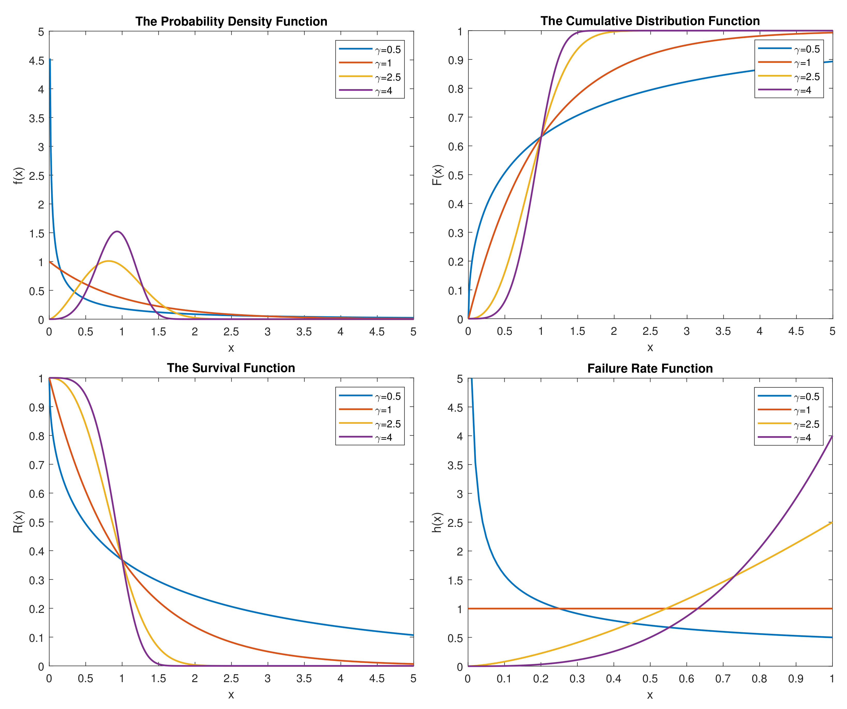
Figure 1 shows the different representative plots of f ( x ) , F ( x ) , R ( x ) = 1 F ( x ) and h ( x ) for WEI ( δ , γ ) given δ = 1 . The shape of the WEI ( δ , γ ) failure rate function depends upon the value of the shape parameter, γ . When γ > 1 , the failure rate is increasing and concave up. When γ < 1 , the failure rate is decreasing and concave up. When γ = 1 , it reduces to a horizontal line that is the failure rate shape of the well-known conventional exponential distribution. Due to the flexibility of the failure rate function, WEI ( δ , γ ) has been proposed in statistics literature to analyze real applications for industrial and engineering reliability inference and medical survival analysis.
This distribution was introduced by Weibull [1]. Since then, it has been one of most important probability models for lifetime distributions. Abernethy [2] produced a Handbook for WEI ( δ , γ ) . Zhang et al. [3] studied the weighted least square estimation for the parameters. Al Omari and Ibrahim [4] investigated Bayesian survival estimation utilizing censored data from WEI ( δ , γ ) . Technology advancement prolongs the process of collecting a random sample of lifetimes. To shorten the process of collecting a sample, many censoring schemes have been cooperated to develop the parameter inference of WEI ( δ , γ ) . Wu [5] developed the point and interval estimations for WEI ( δ , γ ) parameters by using the maximum likelihood procedure under a progressive censoring. Zhang and Xie [6] analyzed the reliability and maintainability based on the upper truncated sample from WEI ( δ , γ ) . Ahmed [7] investigated Bayes estimation by means of the balanced square error loss function under the progressive type-II censoring. Murthy et al. [8] provided many useful modelings of WEI ( δ , γ ) until 2003. In this paper, the estimation methods for any function of the unknown rate parameter, δ , are considered based on a progressive type-II censored sample that can be obtained via the progressive type-II censoring scheme during the life test. The progressive type-II censoring scheme can be implemented as follows. At the beginning of the experiment, all n subjects are under the treatment simultaneously at the time labeled by X 0 : s : n = 0 . Once the ith failure time, X i : s : n , is observed, R i items will be randomly withdrawn from the remaining survival items, for i = 1 , 2 , 3 , , s where 1 s n and R i , i = 1 , 2 , 3 , , s are determined before the experiment based on administrative concern. Then the observed failure data set, which contains X i : s : n , i = 1 , 2 , 3 , , s , is called the progressively type-II censored sample under the progressive type-II censoring scheme, R i , i = 1 , 2 , 3 , , s .
Recently, Han [9] studied the structure of the hierarchical prior distribution and a new Bayesian estimation, which is called the Expected Bayesian or E-Bayesian method. Han [10] compared the E-Bayesian estimation method and hierarchical Bayesian estimation for the system failure rate by utilizing the quadratic loss function and established the E-Bayesian estimation properties under three different priors for hyper-parameters. Jaheen and Okasha [11] obtained the E-Bayesian inference of the outer power parameter and reliability from a Burr type-XII distribution with type-II censoring based on squared error loss (SEL) and LINEX loss functions. Okasha [12] computed the E-Bayesian estimates for the unknown rate parameter, reliability (parallel and series systems) and failure rate functions using the SEL function based on type-II censored samples from WEI ( δ , γ ) . Okasha [13] suggested using a balanced SEL function for the Bayesian estimation of the unknown power parameter and reliability of a Lomax distribution with type-II censored data. Okasha and Wang [14] provided the geometric model to E-Bayesian estimation for the unknown parameters based on record statistics using different balance loss functions. Okasha et al. [15] investigated E-Bayesian point and interval predictions when only outer power parameter unknown based on type-II censored with two samples from the Burr XII distribution. The aforementioned references have the common conclusion that indicates that the E-Bayes estimate method provides better estimation than the Bayes estimate method does. Other work on E-Bayesian estimation of parameters under different loss functions can be seen in [16,17,18,19].
A scenario throughout this paper is discussing the E-Bayesian estimates of any function of unknown rate parameter, which includes rate parameter, reliability, failure rate and quantile functions as special cases, based on the progressively type-II censored sample. In Section 2, the Bayesian and non-Bayesian estimators will be presented for any given function of rate parameter. Section 3 presents the expected Bayesian or E-Bayesian estimation methods for any given function of rate parameter under three priors for the hyper-parameters. The properties of the E-Bayesian estimators under the SEL function are developed for four special functions in Section 4. In Section 5, a simulation study will be conduced to compare the performance of the different estimators. In the following, two real data sets, one is regarding the remission times from 128 bladder cancer patients reported by Lee and Wang [20] and the other is about the breaking stresses of carbon fibers used in the fibrous composite materials reported by Padgett and Spurrier [21], will be used for the application illustration. Finally, Section 7 provides some concluding remarks.

2. Model and Estimations for η ( δ )

Given a progressively censored sample, X i : s : n , i = 1 , 2 , 3 , , s , under the progressive type-II censoring R i , i = 1 , 2 , 3 , , s , it is noted that X i 1 : s : n < X i : s : n , i = 1 , 2 , 3 , , s and n = s + i = 1 s R i . In this section, the progressively type-II censored sample, X i : s : n , i = 1 , 2 , 3 , , s , is taken via the life test on n items of which lifetimes follow the WEI ( δ , γ ) . Let Φ = X i : s : n , R i , i = 1 , 2 , 3 , , s . Then the likelihood function can be presented as follows
L ( δ , γ Φ ) = c i = 1 s f ( X i : s : n ; δ , γ ) 1 F ( x i : s : n ; δ , γ ) R i = c δ s ψ ( γ ; Φ ) e δ D ,
where
c = n ( n 1 R 1 ) ( n R 1 R s 1 s + 1 ) , ψ ( γ ; Φ ) = γ s i = 1 s X i : s : n γ 1 ,
and
D D ( γ ; Φ ) = i = 1 s ( R i + 1 ) X i : s : n γ .
The next example shows that the aforementioned progressively type-II censored sample contains the type-II censored and complete samples as two special cases.
Example 1.
Let X i : s : n , i = 1 , 2 , 3 , , s be a progressively censored sample under the progressive type-II censoring R i , i = 1 , 2 , 3 , , s , then
[1] 
If R 1 = R 2 = = R s 1 = 0 , and R s = n s then the aforementioned censoring is the type-II censoring (see Okasha [12]).
[2] 
If R 1 = R 2 = = R s = 0 , and n = s then the aforementioned censored sample corresponds to the complete sample.
Bayesian estimation based on the type-II censored sample from WEI ( δ , γ ) has been studied by Canavos and Tsokos [22], Panahi and Asadi [23] and Singh et al. [24]. In these three referenced papers, gamma or inverted gamma distributions have been used as the prior of the rate parameter or scale parameter, and uniform or gamma distributions have been used as the prior for the shape parameter. Other possible joint priors used were Jeffery priors without hyper-parameters. Whenever a prior is used for the shape parameter in Bayesian estimation for WEI ( δ , γ ) , it raises the level of computational complexity and it is intractable for getting a closed form of the Bayesian estimate. Moreover, the selection of the hyper-parameters for the Bayesian estimation is an important issue. In the current study, we will utilize the E-Bayesian method to investigate the impact of the hyper-parameters to the Bayesian estimate method given a progressively type-II censored sample from WEI ( δ , γ ) . However, there is no closed form for the Bayesian estimate of the shape parameter. Hence, the shape parameter, γ , is treated as a known constant in WEI ( δ , γ ) and the estimation procedure for any given function, η ( δ ) , of the rate parameter, δ , will be focused on in this study. The given function, η ( δ ) , includes the identity function, δ , the reliability, R t = e δ t γ , hazard rate function, h ( t ; δ , γ ) = δ γ t γ 1 , and quantile function, ξ ( p ; δ , γ ) = ln ( 1 p ) 1 / γ δ 1 / γ , where 0 < p < 1 , as special cases. First, the maximum likelihood estimator (MLE) of δ can be obtained as
δ ^ M L = s D
and the MLE of η ( δ ) is obtained by the plugging in method and can be denoted by η ^ = η ( δ ^ M L ) . For getting the Bayesian estimation of η ( δ ) under the SEL function, the gamma conjugate prior of the unknown rate parameter δ ,
P ( δ | β , ρ ) = ρ β Γ ( β ) δ β 1 e δ ρ , δ > 0 ,
where β > 0 and ρ > 0 are hyper-parameters, will be used in this study. Combining Equation (4) with Equation (6), the posterior density of δ can be presented as
q ( δ Φ ) = A δ s + β 1 e ( ρ + D ) δ , δ > 0 ,
where
A = ( ρ + D ) s + β Γ ( s + β ) .
Under the SEL function, the Bayesian estimate of η ( δ ) can be given as E ( η ( δ ) Φ ) where E ( · Φ ) is taking the posterior expectation. When η ( δ ) = δ , the Bayesian estimate, E ( η ( δ ) Φ ) , is given as,
δ ^ B S ( β , ρ ) = s + β ρ + D ,
that is, the posterior mean of (7). When η ( δ ) = e δ t γ , the Bayes estimate, E ( η ( δ ) Φ ) , can be obtained as
R ^ B S ( t ) = ρ + D ρ + D + D * s + β ,
where D * = t γ . When η ( δ ) = δ γ t γ 1 , the Bayes estimate, E ( η ( δ ) Φ ) , can be shown as
h ^ B S ( t ) = γ t γ 1 s + β ρ + D .
When η ( δ ) = ln ( 1 p ) 1 / γ δ 1 / γ , the Bayes estimate, E ( η ( δ ) Φ ) , can be derived as,
ξ ^ B S ( p ) = Γ ( s + β 1 / γ ) Γ ( s + β ) ln ( 1 p ) 1 / γ ( ρ + D ) 1 / γ , 0 < p < 1 .
Hence, the Bayesian estimate of η ( δ ) is a function of hyper-parameters, β and ρ , and is denoted by η ^ B S ( β , ρ ) . To deal with the selection of these two hyper-parameters, the following E-Bayesian estimation method will be discussed.

3. E-Bayesian Estimation for η ( δ )

Taking the suggestion by Han [9], the hyper-parameters, β and ρ , are selected to guarantee that the prior P ( δ | β , ρ ) in (6) is a decreasing function of δ . The derivative of P ( δ | β , ρ ) , with respect to δ , is
d P ( δ ) d δ = ρ β Γ ( β ) δ β 2 e δ ρ [ ( β 1 ) δ ρ ] .
Thus, for 0 < β < 1 , ρ > 0 and δ > 0 , the prior P ( δ | β , ρ ) is a decreasing function of δ . Assume that the hyper-parameters β and ρ are independent random variables and have density functions, π 1 ( β ) and π 2 ( ρ ) , respectively. Then the join bivariate density function of β and ρ can be represented,
π ( β , ρ ) = π 1 ( β ) π 2 ( ρ ) .
The E-Bayesian estimate of η ( δ ) considered in the current research is defined as the expectation of the Bayesian estimate, η ^ B S ( β , ρ ) , with respect to the joint prior distribution of the hyper-parameters and can be expressed as
η ^ E B = ϱ η ^ B S ( β , ρ ) π ( β , ρ ) d β d ρ ,
where ϱ is the domain of β and ρ such that the prior density is decreasing in δ and η ^ B S is the Bayes estimate of η ( δ ) evaluated respectively via (8), (9), (10) or (11) for η ( δ ) = δ , η ( δ ) = R ( t ) , η ( δ ) = h ( t ; δ , γ ) or η ( δ ) = ξ ( p ; δ , γ ) as special cases. For more details about E-Bayesian, readers may refer to References [10,11,12,13,14,15,16,17].
The properties of the E-Bayesian estimate of η ( δ ) rely on different joint priors of the hyper-parameters β and ρ . In order to investigate the E-Bayesian estimation of η ( δ ) , we use the following three joint priors,
π 1 ( β , ρ ) = 1 a B ( r , v ) β r 1 ( 1 β ) v 1 , 0 < β < 1 , 0 < ρ < a , π 2 ( β , ρ ) = 2 a 2 B ( r , v ) ( a ρ ) β r 1 ( 1 β ) v 1 , 0 < β < 1 , 0 < ρ < a , π 3 ( β , ρ ) = 2 ρ a 2 B ( r , v ) β r 1 ( 1 β ) v 1 , 0 < β < 1 , 0 < ρ < a . ,
where r > 0 , v > 0 and B ( r , v ) is the beta function. Therefore, the E-Bayesian estimators of the η ( δ ) under the SEL function can be evaluated as follows,
η ( δ ) ^ E B S 1 = ϱ η ^ B S ( β , ρ ) π 1 ( β , ρ ) d ρ d β = 1 a B ( r , v ) 0 1 0 a η ^ B S ( β , ρ ) β r 1 × ( 1 β ) v 1 d ρ d β
η ( δ ) ^ E B S 2 = ϱ η ^ B S ( β , ρ ) π 2 ( β , ρ ) d ρ d β = 2 a 2 B ( r , v ) 0 1 0 a η ^ B S ( β , ρ ) ( a ρ ) β r 1 × ( 1 β ) v 1 d ρ d β
and
η ( δ ) ^ E B S 3 = ϱ η ^ B S ( β , ρ ) π 3 ( β , ρ ) d ρ d β = 2 a 2 B ( r , v ) 0 1 0 a η ^ B S ( β , ρ ) ρ β r 1 × ( 1 β ) v 1 d ρ d β
Again, the closed form of η ^ B S ( β , ρ ) is needed to establish the properties of the E-Bayesian estimate of η ( δ ) . Therefore, the aforementioned four different functions of η ( δ ) will be used for discussions

3.1. E-Bayesian Estimation for η ( δ ) = δ

Therefore, the E-Bayesian estimators of η ( δ ) = δ under the SEL function can be obtained by plugging (8) into (14), (15) and (16) to respectively produce the following,
δ ^ E B S 1 = ϱ δ ^ B S ( β , ρ ) π 1 ( β , ρ ) d ρ d β = 1 a B ( r , v ) 0 1 0 a s + β ρ + D β r 1 ( 1 β ) v 1 d ρ d β = 1 a s + r r + v ln D + a D ,
δ ^ E B S 2 = 2 a s + r r + v D + a a ln D + a D 1 ,
and
δ ^ E B S 3 = 2 a s + r r + v 1 D a ln D + a D .

3.2. E-Bayesian Estimation for η ( δ ) = e δ t γ

The E-Bayesian estimation of the reliability, η ( δ ) = R ( t ) , under the SEL function can be derived by plugging (9) into (14), (15) and (16) to respectively produce the following,
R ^ E B S 1 = ϱ R ^ B S ( t ) π 1 ( β , ρ ) d ρ d β = 1 a B ( r , v ) 0 1 0 a ρ + D ρ + D + D * s + β β r 1 ( 1 β ) v 1 d ρ d β . = 1 a B ( r , v ) 0 a ρ + D ρ + D + D * s 0 1 e β ln ρ + D ρ + D + D * β r 1 ( 1 β ) v 1 d β d ρ = 1 a 0 a ρ + D ρ + D + D * s F 1 : 1 r ; r + v ; ln ρ + D ρ + D + D * d ρ ,
R ^ E B S 2 = 2 a 2 0 a ( a ρ ) ρ + D ρ + D + D * s F 1 : 1 r ; r + v ; ln ρ + D ρ + D + D * d ρ ,
and
R ^ E B S 3 = 2 a 2 0 a ρ ρ + D ρ + D + D * s F 1 : 1 r ; r + v ; ln ρ + D ρ + D + D * d ρ ,
where F 1 : 1 . , . ; . is the generalized hyper-geometric function (see Gradshteyn and Ryzhik [25], formula 3.383(1), page 347). Equations (20)–(22) cannot be computed analytically. Therefore, the mathematical packages in Matlab will be used to evaluate those equations.

3.3. E-Bayesian Estimation for η ( δ ) = δ γ t γ 1

The closed form of the E-Bayesian estimation for η ( δ ) = h ( t ) will be obtained in this subsection by plugging (10) into (14), (15) and (16) to respectively produce the following,
h ^ E B S 1 = ϱ h ^ B S ( t ) π 1 ( β , ρ ) d ρ d β = 1 a B ( r , v ) 0 1 0 a γ t γ 1 s + β ρ + D β r 1 ( 1 β ) v 1 d ρ d β = γ t γ 1 a B ( r , v ) 0 1 0 a s + β ρ + D β r 1 ( 1 β ) v 1 d ρ d β = γ t γ 1 a s + r r + v ln a + D D ,
h ^ E B S 2 = 2 γ t γ 1 a s + r r + v a + D a ln a + D D 1 ,
and
h ^ E B S 3 = 2 γ t γ 1 a s + r r + v 1 D a ln a + D D .

3.4. E-Bayesian Estimation for η ( δ ) = ξ ( p ; δ , γ )

The closed form of the E-Bayesian estimation for η ( δ ) = ξ ( p ; δ , γ ) will be obtained in this subsection by plugging (11) into (14), (15) and (16) to respectively obtain the following,
ξ ^ E B S 1 = ϱ ξ ^ B S ( t ) π 1 ( β , ρ ) d ρ d β = ( ln ( 1 p ) ) 1 / γ 1 a B ( r , v ) 0 1 0 a ( ρ + D ) 1 / γ Γ ( s + β 1 / γ ) Γ ( s + β ) β r 1 × ( 1 β ) v 1 d ρ d β = ( ln ( 1 p ) ) 1 / γ 1 a B ( r , v ) 0 a ( ρ + D ) 1 / γ d ρ 0 1 Γ ( s + β 1 / γ ) Γ ( s + β ) β r 1 × ( 1 β ) v 1 d β = ( ln ( 1 p ) ) 1 / γ 1 a B ( r , v ) γ ( a + D ) 1 γ + 1 D 1 γ + 1 γ + 1 ϖ ( s , γ )
ξ ^ E B S 2 = ( ln ( 1 p ) ) 1 / γ 2 a 2 B ( r , v ) γ γ ( a + D ) 1 γ + 2 D 1 γ + 1 ( 2 a γ + a + γ D ) 2 γ 2 + 3 γ + 1 ϖ ( s , γ )
and
ξ ^ E B S 3 = ( ln ( 1 p ) ) 1 / γ 2 a 2 B ( r , v ) γ ( a γ + a γ D ) ( a + D ) 1 γ + 1 + γ D 1 γ + 2 2 γ 2 + 3 γ + 1 ϖ ( s , γ )
where
ϖ ( s , γ ) = 0 1 Γ ( s + β 1 / γ ) Γ ( s + β ) β r 1 ( 1 β ) v 1 d β

4. Properties of E-Bayesian Estimations of η ( δ )

In order to investigate properties of E-Bayesian estimations of η ( δ ) , a specific functional structure is needed. In this section, the functional structures will be focused on the aforementioned four functions. Some relationships among δ ^ E B S j , R ^ E B S j , h ^ E B S j and ξ ^ E B S j ( j = 1 , 2 , 3 ) estimators will be established in this section.
Proposition 1.
Given 0 < a < D , r > 0 , v > 0 , let δ ^ E B S j , j = 1 , 2 , 3 be respectively given by (17), (18) and (19). Then
(i) 
δ ^ E B S 2 < δ ^ E B S 1 < δ ^ E B S 3 and
(ii) 
lim D δ ^ E B S 1 = lim D δ ^ E B S 2 = lim D δ ^ E B S 3 .
Proof of Proposition 1.
(i) From (17), (18) and (19), we have
δ ^ E B S 2 δ ^ E B S 1 = δ ^ E B S 1 δ ^ E B S 3 = 1 a s + r r + v a + 2 D a ln D + a D 2 .
For 1 < x < 1 , we have
ln ( 1 + x ) = x x 2 2 + x 3 3 x 4 4 + = k = 1 ( 1 ) k 1 x k k .
Let x = a D , when 0 < a < D , 0 < a D < 1 , we get
a + 2 D a ln D + a D 2 = a + 2 D a a D 1 2 a D 2 + 1 3 a D 3 1 4 a D 4 + 1 5 a D 5 2 = a D 1 2 a D 2 + 1 3 a D 3 1 4 a D 4 + 1 5 a D 5 2 + 2 a D + 2 3 a D 2 2 4 a D 3 + 2 5 a D 4 = a 2 6 D 2 a 3 6 D 3 + 3 a 4 6 D 4 2 a 5 15 D 5 + = a 2 6 D 2 1 a D + a 4 60 D 4 9 8 a D + > 0 .
According to (29) and (30), we have
δ ^ E B S 2 δ ^ E B S 1 = δ ^ E B S 1 δ ^ E B S 3 > 0 ,
that is
δ ^ E B S 3 < δ ^ E B S 1 < δ ^ E B S 2 .
(ii) From (29) and (30), we get
lim D δ ^ E B S 2 δ ^ E B S 1 = lim D δ ^ E B S 1 δ ^ E B S 3 = 1 a s + r r + v lim D a 2 6 D 2 1 a D + a 4 60 D 4 9 8 a D + = 0 .
That is, lim D δ ^ E B S 1 = lim D δ ^ E B S 2 = lim D δ ^ E B S 3 .
Thus, the proof is complete. □
Remark 1.
The first conclusion of Proposition 1 provides the comparison among E-Bayesian estimations δ ^ E B S j for j = 1 , 2 , 3 . D presents the data information that includes the number of observed failure times. Actually, D is equivalent to the number of items under the life test approaches to infinity. Therefore, the second conclusion of Proposition 1 implies that δ ^ E B S j for j = 1 , 2 , 3 are asymptotically equivalent when the number of items under the life test approaches to infinity.
Proposition 2.
Given 0 < a < D , r > 0 , v > 0 , let R ^ E B S j , j = 1 , 2 , 3 be respectively given by (20), (21) and (22). Then
lim D R ^ E B S 1 = lim D R ^ E B S 2 = lim D R ^ E B S 3 .
Proof of Proposition 2.
From (20), (21) and (22), we get
lim D R ^ E B S 3 R ^ E B S 1 = lim D R ^ E B S 1 R ^ E B S 2 = lim D { 1 a 2 0 a 2 ρ a ρ + D ρ + D + D * s × F 1 : 1 r , r + v ; ln ρ + D ρ + D + D * d ρ } = 0 .
That is, lim D R ^ E B S 1 = lim D R ^ E B S 2 = lim D R ^ E B S 3 .
Thus, the proof is complete. □
Remark 2.
More detail information about the integral results provided by (20), (21) and (22) is needed to compare these three E-Bayesian estimates of reliability. But currently it is not available. Proposition 2 shows that all R ^ E B S j , j = 1 , 2 , 3 are asymptotically equivalent when the number of items under the life test approaches to infinity.
Proposition 3.
Given 0 < a < D , r > 0 , v > 0 , let h ^ E B S j , j = 1 , 2 , 3 be respectively given by (23), (24) and (25). Then
(i) 
h ^ E B S 3 < h ^ E B S 1 < h ^ E B S 2 and
(ii) 
lim D h ^ E B S 1 = lim D h ^ E B S 2 = lim D h ^ E B S 3 .
Proof of Proposition 3.
(i) From (23), (24) and (25), we have
h ^ E B S 2 h ^ E B S 1 = h ^ E B S 1 h ^ E B S 3 = γ t γ 1 1 a r + r r + v a + 2 D a ln D + a D 2 .
According to (30) and (31), we obtain
h ^ E B S 2 h ^ E B S 1 = h ^ E B S 1 h ^ E B S 3 > 0 ,
that is
h ^ E B S 3 < h ^ E B S 1 < h ^ E B S 2 .
(ii) From (30) and (31), we get
lim D h ^ E B S 2 h ^ E B S 1 = lim D h ^ E B S 1 h ^ E B S 3 = γ t γ 1 1 a r + r r + v × lim D a 2 6 D 2 1 a D + a 4 60 D 4 9 8 a D + = 0 .
That is, lim D h ^ E B S 1 = lim D h ^ E B S 2 = lim D h ^ E B S 3 .
The proof is complete. □
Remark 3.
The first result of Proposition 3 gives the comparison among E-Bayesian estimations h ^ E B S j for j = 1 , 2 , 3 and the second result of Proposition 3 implies that all h ^ E B S j for j = 1 , 2 , 3 are asymptotically equivalent when the number of items under the life test approaches to infinity.
Proposition 4.
Given 0 < a < D , r > 0 , v > 0 , let ξ ^ E B S j , j = 1 , 2 , 3 be respectively given by (26), (27) and (28). Then
(i) 
ξ ^ E B S 2 < ξ ^ E B S 1 < ξ ^ E B S 3 and
(ii) 
lim D ξ ^ E B S 1 = lim D ξ ^ E B S 2 = lim D ξ ^ E B S 3 .
Proof of Proposition  4.
(i) From (26), (27) and (28), we get
ξ ^ E B S 3 ξ ^ E B S 1 = ξ ^ E B S 1 ξ ^ E B S 2 = ( ( ln ( 1 p ) ) ) 1 / γ a 2 0 a 2 ρ a ( ρ + D ) 1 / γ d ρ × 1 B ( r , v ) 0 1 Γ ( s + β 1 / γ ) Γ ( s + β ) β r 1 ( 1 β ) v 1 d β > 0 .
It is because
0 a ( a 2 ρ ) ( ρ + D ) 1 / γ d ρ = γ D 1 + 1 / γ ( 2 γ ( a + D ) + a ) + γ ( a + D ) 1 + 1 / γ ( a 2 γ D ) ( γ + 1 ) ( 2 γ + 1 ) < 0 , D > 0
(ii) The following results can also be obtained
lim D γ D 1 + 1 / γ ( 2 γ ( a + D ) + a ) + γ ( a + D ) 1 + 1 / γ ( a 2 γ D ) ( γ + 1 ) ( 2 γ + 1 ) = 0 .
That is, lim D ξ ^ E B S 1 = lim D ξ ^ E B S 2 = lim D ξ ^ E B S 3 . Thus, the proof is complete. □
Remark 4.
The first conclusion of Proposition 4 provides the comparison among E-Bayesian estimations ξ ^ E B S j for j = 1 , 2 , 3 and the second conclusion of Proposition 4 implies that all ξ ^ E B S j for j = 1 , 2 , 3 are asymptotically equivalent when the number of items under the life test approaches to infinity.

5. Simulation Study and Comparisons

The closed forms of mean square error (MSE) and bias for the E-Bayesian estimators considered in this study are not available. Therefore, a simulation study will be conducted to compare the performance of all aforementioned estimators for δ , R ( t ) , h ( t ) and ξ ( p ) , respectively, in terms of the computed mean square error (MSE). The simulation study has the following inputs: three different progressive type-II censoring schemes (Schs),
  • Sch 1: R 1 = · · · = R s 1 = 0 a n d R s = n s ,
  • Sch 2: R 1 = · · · = R s 1 = 1 a n d R s = n 2 s + 1 ,
  • Sch 3: R 1 = R 2 = · · · = R s = ( n s ) / s ;
Weibull distribution parameters, ( δ , γ ) = ( 1.0 , 1.5 ) or ( δ , γ ) = ( 0.9 , 2.0 ) ; sample size, n = 30 , 70 , 150 ; the number of observed failure times, s = 10 , 30 , 45 , 70 , 100 , 150 . In order to obtain Bayesian estimates of δ , R ( t ) , h ( t ) and ξ ( p ) , the hyper-parameters of the gamma prior for δ used are with ( β , ρ ) = ( 0.9 , 0.5 ) or ( β , ρ ) = ( 0.5 , 0.5 ) . Moreover, E-Bayesian estimates of δ , R ( t ) , h ( t ) and ξ ( p ) will be derived by using the beta distribution with ( r , v ) = ( 0.5 , 0.5 ) or ( r , v ) = ( 3.0 , 4.0 ) as the prior of the hyper-parameter, β and the prior distribution with a = 1.5 or a = 6 for the hyper-parameter, ρ . The steps of the simulation study are addressed next.

Simulation Study

Given n subjects for the life test experiment, the number of observed failure times, s ( n ) , a progressive type-II censoring scheme mentioned above, a pair of Weibull distribution parameters, ( δ , γ ) , a pair of ( β , ρ ) , a value of a and a pair of ( r , v ) , the simulation is conducted according to the following steps:
  • A progressive type-II sample with n test items and s observed failure times is generated from WEI( δ , γ ) by implementing the progressive type-II censoring R i , i = 1 , 2 , 3 , , s using a MATLAB program that was developed by the authors.
  • The MLE δ ^ M L can be obtained by Equation (5), and the MLEs of R ( t ) , h ( t ) and ξ ( p ) can be obtained by plugging δ ^ M L into R ( t ) , h ( t ) and ξ ( p ) , respectively.
  • Under the SEL function, the Bayesian estimates δ ^ B S , R ^ B S , h ^ B S and ξ ^ B S are calculated by plugging the given paired of ( β , ρ ) in Equations (8)–(11), respectively.
  • Under the SEL function, the E-Bayesian estimates, δ ^ E B S i , i = 1 , 2 , 3 , are computed through Equations (17)–(19).
  • Under the SEL function, the E-Bayesian estimates R ^ E B S i , i = 1 , 2 , 3 , are computed through Equations (20)–(22).
  • Under the SEL function, the E-Bayesian estimates h ^ E B S i , i = 1 , 2 , 3 , are computed through Equations (23)–(25).
  • Under the SEL function, the E-Bayesian estimates ξ ^ E B S i , i = 1 , 2 , 3 , are computed through Equations (26)–(28).
  • Repeat Step 1 to Step 7 10,000 times and 10,000 estimates from Step 2 to Step 7 are respectively calculated.
The above simulation was carried out by using a MATLAB program. Let Θ = ( θ 1 , θ 2 , θ 3 , θ 4 ) = ( δ , R ( t ) , h ( t ) , ξ ( p ) ) and Θ ^ j = ( θ ^ 1 , j , θ ^ 2 , j , θ ^ 3 , j , θ ^ 4 . j ) for j = 1 , 2 , , 10 , 000 be the corresponding 10,000 estimates for any estimator mentioned in the simulation study. Then, we calculated the average value estimates (AVEs) as θ ^ ¯ i = 1 10 , 000 j = 1 10 , 000 θ ^ i , j and mean square errors (MSEs) to be 1 10 , 000 j = 1 10 , 000 ( θ ^ i , j θ i ) 2 for i = 1 , 2 , 3 , 4 , respectively. The simulation results are given in Table 1 and Table 2 that show the following observations:
(1)
The respective average estimate (AVE) and mean square error (MSE) from 10,000 estimates of each different estimator decrease as n increases.
(2)
The AVE and MSE of each different estimator decrease as a increases.
(3)
The AVE and MSE of each different estimator in Prior II are less than Prior I.
(4)
The E-Bayesian estimators of the scale parameter, δ , the reliability, R, failure rate and h functions perform better than Bayesian estimators in terms of minimum MSE and AVE.
(5)
The E-Bayesian estimators of δ , R and h have the minimum MSE among all other estimators.
(6)
The E-Bayesian estimators of δ , R and h using prior distribution perform better than other estimators in terms of minimum MSE.
(7)
The E-Bayesian estimators of δ , R and h based on the SEL loss function under prior distribution have the minimum MSE compared with all other estimators.
(8)
All estimators for the median lifetime are very competitive in terms of MSE under each combination of the simulation inputs.
Therefore, we recommend to use the E-Bayesian procedure to estimate the parameters δ , R, h and ξ when type-II censoring scheme is used for life test because of the better performance over the other estimates in terms of minimum MSE.

6. Applications to Real Data

In this section, two real data sets will be used for the E-Bayesian estimation application. The first data set, that was originally reported by Lee and Wang [20], contains the remission times (in months) of 128 bladder cancer patients. The second data set, that was originally reported by Padgett and Spurrier [21], is regarding breaking stresses (in GPa) of carbon fibers of a certain type used in fibrous composite materials. For easy reference, both complete data sets are also reported in Table 3 and Table 4, respectively. Before the E-Bayesian estimation procedure is applied to these two data sets, a Kolmogorov–Smirnov (K-S) test and the scaled total time on test (TTT) plot mentioned by Aarset [26] will be applied to examine these two data sets. Since the K-S test can be conducted through current existing software, the scaled TTT transform will be addressed briefly in this section. The scaled TTT transform is defined as T ( t ) = H 1 ( t ) / H 1 ( 1 ) where H 1 ( t ) = 0 t R ( u ) d u and 0 t 1 . The corresponding empirical scaled TTT transform will be addressed by g ( r / n ) = H n 1 ( r / n ) / H n 1 ( 1 ) where H n 1 ( r / n ) = i = 1 r X ( i ) + ( n r ) X ( r ) , H n 1 ( 1 ) = i = 1 n X ( i ) , X ( i ) , i = 1 , 2 , , n denotes the ordered statistic of the lifetime sample X 1 < X 2 < < X n and r = 1 , 2 , 3 , , n . Then the empirical scaled TTT plot will be ( x , g ( x ) ) | 0 x 1 . Aarset [26] mentioned that the scaled TTT transform is convex (concave) if the hazard function decreases (increases) and the hazard function is a bathtub (unimodal) if the scaled TTT transform changes from convex (concave) to concave (convex).

6.1. Example 1

First, we use the data set from Table 3 to fit with WEI ( δ , γ ) . The MLEs of the unknown δ and γ of WEI ( δ , γ ) are given by δ ^ = 0.0939 and γ ^ = 1.0478 
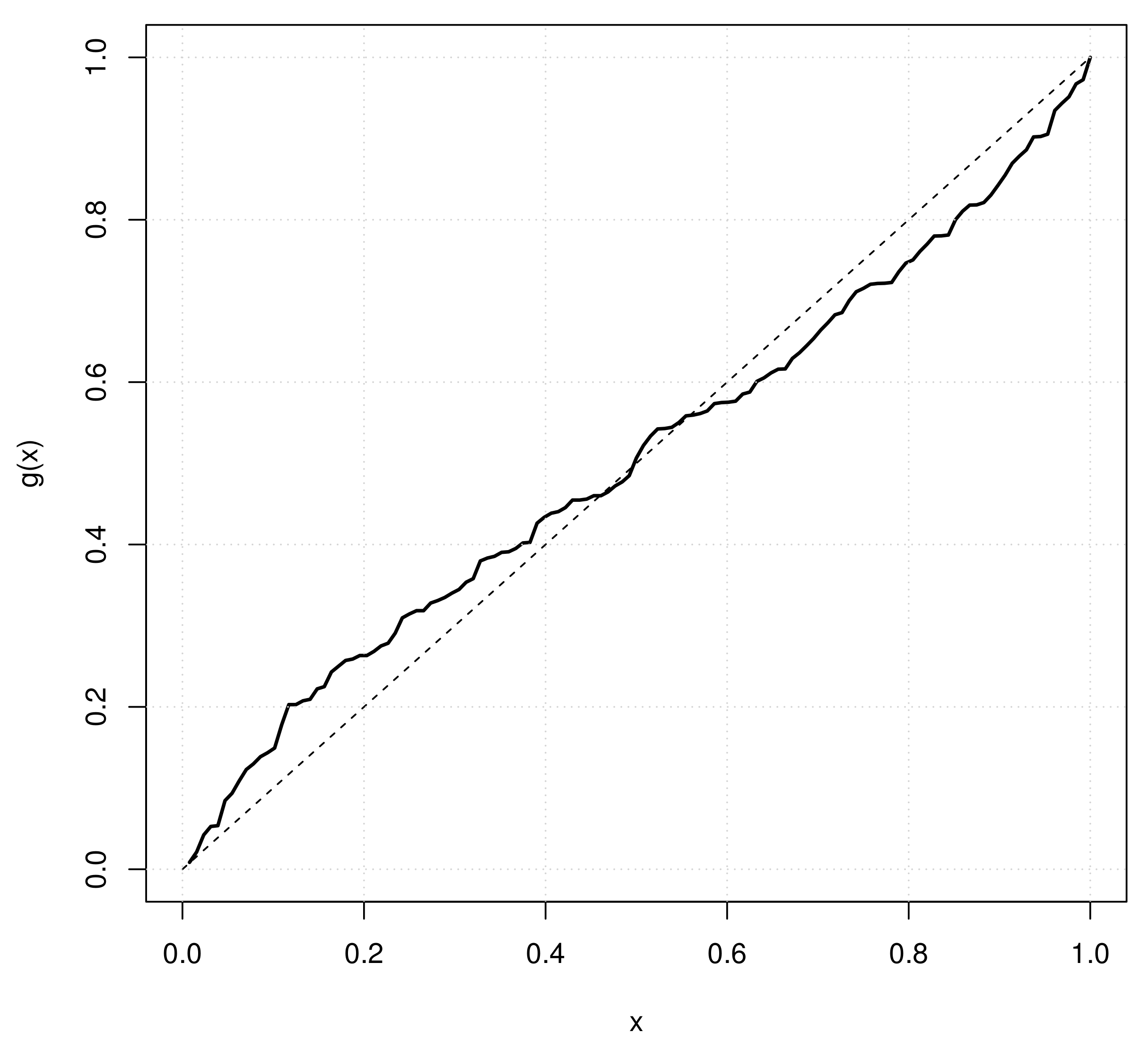
. By using the K-S test with a significance level of 0.05, the test statistic value is 0.069449 with p-value = 0.5675. Figure 2 shows the empirical scaled TTT plot of the 128 remission times of bladder cancer patients and indicates concave on the left lower part and slightly curved up on the right upper part. The MLE of γ is larger than 1 but very closed to 1, indicating the hazard function is an increasing or constant function. Therefore, based on the K-S test result, it is still reasonable to assume that the Weibull distribution is accepted as a good fit. The true parameters of WEI ( δ , γ ) will be assumed as δ = 0.0939 and γ = 1.0478 in this section for the practical application purpose.
From Table 3, the first 15 ordered statistics or the first 30 ordered statistics will be used as two type-II censored samples with s = 15 and 30, respectively, to obtain the aforementioned estimates of δ , R ( t ) , h ( t ) and ξ ( p ) functions assuming that the shape parameter γ is known as 1.0478. All different estimates of δ , R ( t ) , h ( t ) , ξ ( p ) are calculated and displayed in Table 5, where R ( t ) and h ( t ) functions are estimated at t = 0.9 , ξ ( p ) is estimated at p = 0.5 and Bayes estimates are obtained by using hyper-parameters, β = 0.5 and ρ = 0.5 , for the prior because no other information about the unknown rate parameter of the Weibull distribution is available.

6.2. Example 2

The data set from Table 4 is used to fit WEI ( δ , γ ) and the MLEs of the unknown δ and γ of WEI ( δ , γ ) are obtained as δ ^ = 0.0491 and γ ^ = 2.792 
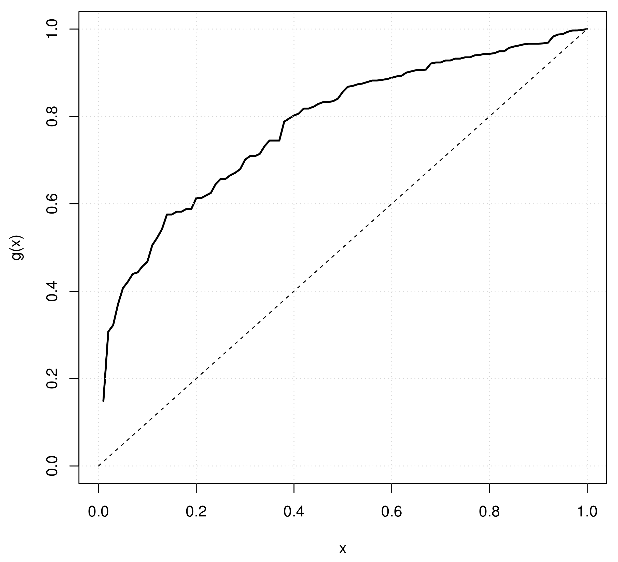
. The K-S test with a significance level of 0.05 provides the test statistic value 0.061136 and p-value = 0.8489. Figure 3 shows the empirical scaled TTT plot of the 100 breaking stresses of carbon fibers and indicates a concave shape. It means that the hazard function is an increasing function and shape parameter γ must be greater than 1. The MLE of γ presents a consistent conclusion. Hence, the Weibull distribution is accepted as a good fit probability model for the carbon fiber breaking stresses. In this application, WEI ( δ , γ ) , with δ = 0.0491 and γ = 2.792 , is assumed as the true distribution for the carbon fiber breaking stresses.
The first 15 ordered statistics or the first 30 ordered statistics in Table 4 are used as two type-II censored samples with s = 15 and 30, respectively. To derive the aforementioned estimates of δ , R ( t ) , h ( t ) and ξ ( p ) functions, we assumed that the shape parameter γ is known as 1.0478. All estimation results for δ , R ( t ) , h ( t ) and ξ ( p ) are calculated and displayed in Table 6, where R ( t ) and h ( t ) functions are estimated at t = 0.9 , ξ ( p ) is estimated at p = 0.5 and Bayes estimates are calculated by using hyper-parameters, β = 0.5 and ρ = 0.5 , for the prior because no other information about the unknown rate parameter of the Weibull distribution is available.

7. Concluding Remarks

Based on the progressively type-II censored sample, the expected Bayesian estimate method, called the E-Bayesian method, for any function of rate parameter has been established by using the square error loss function. The aforementioned function includes the identity function, i.e., rate parameter, reliability, failure rate and quantile functions of the two-parameter Weibull distribution as special cases. Three different priors of the hyper-parameters are introduced to investigate the impact of hyper-parameters on the E-Bayesian estimators. Some theoretical properties among three E-Bayesian estimators for each of these four functions have been derived. The performance comparison among three E-Bayesian, Bayesian and maximum likelihood estimators of the rate parameter, reliability, failure rate and quantile functions is also carried out through a simulation study. Based on the minimum mean square error criterion, the simulation results showed that the E-Bayesian method performs quite well in estimating the rate parameter as well as reliability, failure rate and quantile functions. Finally, two real data sets regarding the remission times from 128 bladder cancer patients and breaking stresses (in GPa) of carbon fibers used in fibrous composite materials were used to demonstrate two-parameter Weibull modeling and to obtain the MLE, Bayesian and E-Bayes estimates for the rate parameter, reliability, failure rate and quantile functions under the SEL function.
The E-Bayesian estimation using different loss functions for reliability characteristics of the two-parameter Weibull distribution under other different censoring schemes as well as theoretical properties of the E-Bayesian estimate for many different families of η ( δ ) functions is interesting and difficult work that needs more time. We are currently working on the corresponding problems.

Author Contributions

Investigation, H.M.O., H.S.M. and Y.L.; methodology, H.M.O., H.S.M. and Y.L.; software, H.M.O., H.S.M. and Y.L.; validation, H.M.O., H.S.M. and Y.L.; writing, H.M.O., H.S.M. and Y.L.; All authors have read and agreed to the published version of the manuscript.

Funding

This research was funded by the Deanship of Scientific Research at Princess Nourah bint Abdulrahman University through the Fast-track Research Funding Program.

Institutional Review Board Statement

Not applicable.

Informed Consent Statement

Not applicable.

Data Availability Statement

Two Data sets are contained within the article or references [20,21].

Acknowledgments

This research was funded by the Deanship of Scientific Research at Princess Nourah bint Abdulrahman University through the Fast-track Research Funding Program. Authors would like to thank the anonymous referees for their suggestions and comments to significantly improve this manuscript.

Conflicts of Interest

The authors declare no conflict of interest.

References

  1. Weibull, W. A Statistical Distribution Function of Wide Applicability. J. Appl. Mech. 1951, 18, 293–297. [Google Scholar] [CrossRef]
  2. Abernethy, R.B. The New Weibull Handbook, 5th ed.; CRC Press: Boca Raton, FL, USA, 2006. [Google Scholar]
  3. Zhang, L.F.; Xie, M.; Tang, L.C. On weighted least square estimation for the parameters of Weibull distribution. In Recent Advances in Reliability and Quality Design; Hoang, P., Ed.; Springer: London, UK, 2008; pp. 57–84. [Google Scholar]
  4. Al Omari, M.A.; Ibrahim, N.A. Bayesian survival estimation for Weibull distribution with censored data. J. Appl. Sci. 2011, 11, 393–396. [Google Scholar]
  5. Wu, S.J. Estimation of the two parameter Weibull distribution with progressive censoring. J. Appl. Stat. 2008, 35, 1139–1150. [Google Scholar] [CrossRef]
  6. Zhang, T.; Xie, M. On the Upper Truncated Weibull Distribution and Its Reliability Implications. Reliab. Syst. Saf. 2011, 96, 194–200. [Google Scholar] [CrossRef]
  7. Ahmed, E.A. Bayesian estimation based on progressive Type-II censoring from two-parameter Weibull model: An Markov chain Monte Carlo approach. J. Appl. Stat. 2014, 4, 752–768. [Google Scholar] [CrossRef]
  8. Murthy, D.N.P.; Xie, M.; Jiang, R. Weibull Models; John Wiley and Sons: New York, NY, USA, 2004. [Google Scholar]
  9. Han, M. The structure of hierarchical prior distribution and its applications. Chin. Oper. Res. Manag. Sci. 1997, 6, 31–40. [Google Scholar]
  10. Han, M. E-Bayesian estimation and hierarchical Bayesian estimation of failure rate. Appl. Math. Model. 2009, 33, 1915–1922. [Google Scholar] [CrossRef]
  11. Jaheen, Z.F.; Okasha, H.M. E-Bayesian estimation for the Burr type XII model based on type-2 censoring. Appl. Math. Model. 2011, 35, 4730–4737. [Google Scholar] [CrossRef]
  12. Okasha, H.M. E-Bayesian Estimation of System Reliability with Weibull Distribution Based on Type-2 Censoring. J. Adv. Res. Sci. Comput. 2012, 4, 33–45. [Google Scholar]
  13. Okasha, H.M. E-Bayesian estimation for the Lomax distribution based on type-II censored data. JOEMS 2014, 22, 489–495. [Google Scholar] [CrossRef] [Green Version]
  14. Okasha, H.M.; Wang, J. E-Bayesian estimation for the geometric model based on record statistics. Appl. Math. Model. 2016, 40, 658–670. [Google Scholar] [CrossRef]
  15. Okasha, H.M.; Wang, C.; Wang, J. E-Bayesian Prediction for the Burr XII Model Based on Type-II Censored Data with Two Samples. Adv. Theor. Phys. 2020. [Google Scholar] [CrossRef]
  16. Okasha, H.M. Estimation for the Exponential Model Based on Record Statistic. J. Stat. Theory Appl. 2019, 18, 236–243. [Google Scholar]
  17. Okasha, H.M.; Mustafa, A. E-Bayesian Estimation for the Weibull Distribution under Adaptive Type-I Progressive Hybrid Censored Competing Risks Data. Entropy 2020, 22, 903. [Google Scholar] [CrossRef] [PubMed]
  18. Algarni, A.; Almarashi, H.M.; Okasha, H.M.; Tony, N.H.K. E-Bayesian Estimation of Chen Distribution Based on Type-I Censoring Scheme. Entropy 2020, 22, 636. [Google Scholar] [CrossRef] [PubMed]
  19. Nassar, M.; Okasha, H.; Albassam, M. E-Bayesian estimation and associated properties of simple step–stress model for exponential distribution based on type-II censoring. Qual. Reliab. Eng. Int. 2021, 37, 997–1016. [Google Scholar] [CrossRef]
  20. Lee, E.T.; Wang, J. Statistical Methods for Survival Data Analysis, 3rd ed.; John Wiley and Sons: Hoboken, NJ, USA, 2003. [Google Scholar]
  21. Padgett, W.J.; Spurrier, J.D. Shewhart-type Charts for Percentiles of Strength Distributions. J. Qual. Technol. 1990, 22, 283–288. [Google Scholar] [CrossRef]
  22. Canavos, G.C.; Tsokos, C.P. Bayesian Estimation of Life Parameters in the Weibull Distribution. Oper. Res. 1973, 21, 755–763. [Google Scholar] [CrossRef]
  23. Panahi, H.; Asadi, S. Estimation of the Weibull Distribution Based on Type-II Censored Samples. Appl. Math. Sci. 2011, 5, 2549–2558. [Google Scholar]
  24. Singh, S.K.; Singh, U.; Sharma, V.K. Bayesian Estimation and Prediction for Flexible Weibull Model under Type-II Censoring Scheme. J. Probab. Stat. 2013, 2013. [Google Scholar] [CrossRef] [Green Version]
  25. Gradshteyn, I.S.; Ryzhik, I.M. Tables of Integrals, Series and Products (Corrected and Enlarged Edition); Academic Press: San Diego, CA, USA, 1980; pp. 96–99. [Google Scholar]
  26. Aarset, M.V. How to identify bathtub hazard rate. IEEE Trans. Reliab. 1987, 36, 106–108. [Google Scholar] [CrossRef]
Figure 1. Plots of PDF, CDF, SF and HRF of the Weibull distribution for various values of γ with δ = 1 .
Mathematics 09 01261 g001
Figure 2. The empirical TTT plot of the remission times from Table 3.
Mathematics 09 01261 g002
Figure 3. The empirical scaled TTT plot of the 100 breaking stresses from Table 4.
Mathematics 09 01261 g003
Table 1. Simulated AVEs (first row) and MSEs (second row) under different settings with δ = 1.0 , γ = 1.5 , p = 0.5 and a = 1.5 .
(n, s)SchemeParMLEPrior IPrior II
BSEBS1EBS2EBS3BSEBS1EBS2EBS3
(20, 5)1 δ 1.24641.27221.12921.19781.06051.18601.11451.18231.0468
0.55070.40710.25790.35230.18310.32390.24810.33830.1770
R0.38980.39990.43980.42380.45580.42390.44380.42780.4598
0.02490.01760.01560.01690.01480.01690.01570.01690.0151
h1.77371.81041.60691.70461.50921.68761.58601.68241.4896
1.11520.82430.52230.71340.37080.65600.50240.68510.3584
ξ 0.76560.81150.88640.85930.91350.85710.89340.86610.9207
0.05240.04850.06280.05950.06750.05870.06510.06140.0703
2 δ 1.25391.27711.13331.20291.06381.19051.11861.18721.0500
0.59740.42310.26890.36930.18940.33720.25870.35480.1831
R0.38910.39930.43930.42330.45530.42340.44330.42730.4593
0.02550.01800.01590.01720.01510.01720.01600.01720.0153
h1.78431.81741.61281.71171.51391.69421.59181.68951.4942
1.20970.85670.54440.74790.38360.68290.52380.71840.3707
ξ 0.76530.81130.88620.85910.91330.85690.89320.86590.9205
0.05370.04970.06400.06080.06870.06000.06630.06270.0715
3 δ 1.24901.27281.12961.19871.06041.18661.11491.18321.0466
0.58270.42170.26850.36710.19040.33660.25840.35270.1841
R0.39080.40090.44080.42480.45670.42490.44470.42880.4607
0.02570.01820.01620.01750.01540.01750.01630.01750.0157
h1.77741.81131.60741.70581.50901.68851.58651.68371.4894
1.17990.85390.54370.74330.38550.68150.52330.71420.3728
ξ 0.76840.81420.88930.86230.91640.86000.89640.86910.9236
0.05450.05070.06560.06220.07040.06140.06800.06430.0732
(30, 10)1 δ 1.10801.13741.06771.09761.03781.09561.06051.09021.0308
0.16630.15850.12110.14100.10400.13880.11860.13780.1021
R0.40740.41090.43260.42400.44110.42410.43480.42630.4433
0.01310.01090.01010.01060.00980.01060.01020.01060.0099
h1.57671.61851.51941.56201.47691.55911.50911.55131.4668
0.33670.32110.24520.28540.21050.28100.24010.27900.2067
ξ 0.77600.79880.83440.82110.84770.82060.83810.82470.8514
0.02690.02600.02940.02870.03050.02860.03000.02920.0312
2 δ 1.11201.14121.07131.10141.04121.09941.06401.09391.0341
0.16850.16120.12300.14320.10550.14100.12040.13990.1036
R0.40630.40990.43160.42300.44010.42310.43380.42530.4424
0.01330.01100.01020.01070.00990.01070.01030.01070.0099
h1.58251.62401.52451.56731.48161.56441.51411.55661.4715
0.34120.32650.24900.28990.21360.28550.24380.28330.2097
ξ 0.77460.79740.83300.81970.84630.81920.83670.82330.8501
0.02720.02620.02950.02880.03060.02870.03010.02930.0313
3 δ 1.10921.13881.06911.09901.03921.09701.06181.09151.0321
0.16090.15480.11800.13730.10140.13520.11550.13410.0995
R0.40650.41020.43180.42330.44040.42330.43410.42550.4426
0.01300.01080.01000.01050.00970.01050.01000.01050.0097
h1.57841.62051.52131.56391.47881.56111.51101.55321.4688
0.32590.31360.23890.27800.20530.27380.23390.27160.2016
ξ 0.77460.79740.83300.81970.84630.81920.83660.82330.8500
0.02650.02550.02880.02810.02990.02800.02940.02860.0306
(45, 15)1 δ 1.07231.09471.04901.06791.03011.06721.04421.06301.0253
0.09220.09220.07610.08410.06910.08360.07500.08270.0682
R0.41210.41410.42890.42310.43480.42310.43050.42470.4364
0.00880.00780.00740.00760.00720.00760.00740.00760.0072
h1.52601.55781.49281.51971.46581.51861.48591.51271.4591
0.18680.18670.15410.17030.13990.16930.15190.16750.1381
ξ 0.77680.79200.81540.80650.82420.80630.81780.80900.8267
0.01800.01750.01890.01860.01940.01860.01920.01890.0197
2 δ 1.07271.09501.04931.06821.03041.06751.04451.06331.0256
0.09250.09240.07630.08430.06920.08380.07520.08290.0683
R0.41200.41400.42880.42300.43470.42300.43040.42460.4363
0.00880.00780.00740.00760.00720.00760.00740.00760.0072
h1.52641.55831.49321.52011.46621.51911.48631.51311.4595
0.18730.18720.15450.17070.14020.16970.15220.16790.1384
ξ 0.77670.79180.81520.80640.82400.80620.81770.80880.8265
0.01800.01750.01890.01860.01940.01860.01920.01880.0197
3 δ 1.06991.09231.04681.06561.02791.06481.04191.06071.0232
0.09140.09140.07560.08340.06870.08290.07450.08210.0679
R0.41290.41480.42970.42390.43550.42390.43130.42540.4371
0.00880.00780.00740.00760.00720.00760.00740.00760.0072
h1.52251.55441.48961.51641.46271.51531.48271.50941.4560
0.18510.18500.15310.16890.13920.16800.15090.16620.1374
ξ 0.77810.79330.81670.80780.82550.80760.81910.81030.8280
0.01820.01770.01920.01890.01970.01890.01950.01910.0200
Table 2. Simulated AVEs (first row) and MSEs (second row) under different settings with δ = 0.9 , γ = 2 , p = 0.5 and a = 3 .
(n, s)SchemeParMLEPrior IPrior II
BSEBS1EBS2EBS3BSEBS1EBS2EBS3
(20, 5)1 δ 1.12181.16010.90650.99170.82131.08150.89470.97890.8106
0.44610.35430.12350.18800.08460.28200.12030.18120.0843
R0.44220.44650.52270.49730.54810.47020.52660.50120.5519
0.02540.01860.01350.01440.01400.01720.01370.01450.0145
h2.01922.08821.63171.78511.47831.94661.61051.76191.4591
1.44531.14800.40010.60920.27400.91380.38970.58710.2732
ξ 0.85550.88340.99810.96021.03600.91971.00410.96601.0422
0.03750.03260.04500.03970.05330.03700.04690.04110.0557
2 δ 1.12851.16470.90930.99530.82321.08580.89750.98240.8125
0.48390.36870.12780.19610.08640.29400.12450.18890.0861
R0.44150.44590.52220.49670.54760.46960.52610.50060.5515
0.02600.01900.01370.01470.01410.01760.01390.01480.0146
h2.03132.09651.63671.79161.48181.95441.61541.76831.4626
1.56781.19460.41420.63530.28000.95260.40330.61220.2790
ξ 0.85510.88300.99780.95991.03580.91941.00380.96571.0420
0.03840.03340.04570.04040.05390.03790.04760.04180.0563
3 δ 1.12411.16080.90640.99200.82071.08210.89460.97910.8101
0.47200.36720.12860.19590.08770.29310.12530.18890.0874
R0.44310.44740.52340.49810.54880.47100.52730.50200.5526
0.02620.01920.01400.01500.01440.01780.01420.01510.0149
h2.02342.08951.63151.78561.47731.94781.61031.76241.4581
1.52911.18960.41670.63480.28420.94970.40590.61200.2832
ξ 0.85760.88541.00020.96231.03800.92181.00620.96811.0443
0.03890.03390.04680.04140.05520.03870.04870.04280.0576
(30, 10)1 δ 0.99721.02960.90520.94760.86270.99180.89900.94110.8568
0.13470.13290.07360.09160.06080.11620.07260.08980.0605
R0.46210.46210.50380.48970.51800.47500.50600.49190.5202
0.01290.01100.00900.00950.00890.01050.00900.00950.0090
h1.79501.85331.62931.70571.55291.78521.61821.69411.5423
0.43640.43060.23840.29670.19700.37640.23510.29090.1959
ξ 0.86790.88140.93860.91920.95790.89930.94170.92230.9611
0.01910.01790.02090.01960.02290.01910.02140.02000.0235
2 δ 1.00081.03310.90800.95070.86520.99520.90180.94420.8594
0.13650.13520.07450.09290.06140.11800.07350.09110.0610
R0.46090.46110.50290.48870.51720.47400.50510.49090.5193
0.01310.01110.00900.00960.00890.01060.00910.00960.0091
h1.80151.85961.63431.71121.55741.79141.62321.69961.5468
0.44220.43790.24150.30110.19890.38250.23800.29520.1977
ξ 0.86660.88020.93740.91810.95680.89810.94050.92110.9600
0.01930.01800.02090.01970.02290.01920.02140.02000.0235
3 δ 0.99831.03090.90630.94880.86390.99300.90020.94240.8580
0.13040.12980.07170.08920.05940.11320.07070.08750.0590
R0.46130.46140.50320.48900.51740.47430.50540.49120.5196
0.01270.01090.00880.00930.00880.01030.00890.00930.0089
h1.79691.85561.63141.70791.55501.78751.62031.69621.5444
0.42230.42050.23240.28910.19240.36670.22920.28340.1913
ξ 0.86670.88030.93750.91810.95680.89810.94060.92120.9600
0.01880.01760.02050.01920.02250.01870.02100.01960.0231
(45, 15)1 δ 0.96510.98890.90690.93500.87870.96400.90270.93070.8747
0.07470.07640.05070.05870.04470.06920.05020.05790.0445
R0.46750.46700.49580.48600.50570.47590.49730.48750.5072
0.00850.00770.00660.00690.00650.00740.00660.00690.0066
h1.73721.78001.63241.68311.58171.73521.62491.67531.5745
0.24210.24750.16420.19020.14480.22410.16260.18750.1441
ξ 0.86980.87870.91690.90390.92990.89060.91890.90590.9320
0.01280.01220.01340.01290.01420.01270.01360.01300.0145
2 δ 0.96540.98920.90710.93530.87900.96430.90300.93100.8749
0.07490.07660.05080.05880.04480.06940.05030.05800.0445
R0.46740.46700.49570.48590.50560.47580.49730.48740.5071
0.00850.00770.00660.00690.00650.00740.00660.00690.0065
h1.73771.78051.63281.68351.58221.73571.62531.67581.5749
0.24280.24810.16450.19060.14500.22470.16280.18790.1443
ξ 0.86970.87860.91670.90370.92970.89040.91880.90580.9319
0.01280.01220.01340.01280.01420.01270.01360.01300.0145
3 δ 0.96290.98670.90500.93300.87700.96190.90080.92870.8729
0.07400.07570.05050.05830.04470.06860.05000.05750.0445
R0.46830.46780.49650.48670.50630.47660.49800.48820.5079
0.00850.00770.00660.00690.00660.00740.00670.00690.0066
h1.73331.77611.62901.67951.57861.73141.62151.67171.5713
0.23990.24520.16360.18900.14470.22230.16200.18640.1441
ξ 0.87090.87980.91790.90490.93090.89160.92000.90700.9330
0.01290.01230.01360.01300.01440.01280.01380.01320.0147
Table 3. The remission times (in months) of 128 bladder cancer patients.
0.080.200.400.500.510.810.901.051.191.26
1.351.401.461.762.022.022.072.092.232.26
2.462.542.622.642.692.692.752.832.873.02
3.703.823.253.313.363.363.483.523.573.64
4.514.873.884.184.234.264.334.344.404.50
5.415.494.985.065.095.175.325.325.345.41
6.977.095.625.715.856.256.546.766.936.94
7.877.937.267.287.327.397.597.627.637.66
9.7410.068.268.378.538.658.669.029.229.47
12.0312.0710.3410.6610.7511.2511.6411.7911.9812.02
12.6313.1113.2913.8014.2414.7614.7714.8315.9616.62
17.1217.1417.3618.1019.1320.2821.7322.6923.6325.74
25.8226.3132.1534.2636.6643.0146.1279.05
Table 4. Breaking stresses (in GPa) of carbon fibers used in fibrous composite materials.
3.702.742.732.503.603.113.272.871.473.11
4.422.413.193.221.693.283.091.873.154.90
3.752.432.952.973.392.982.532.672.933.22
3.392.814.203.332.553.313.312.852.563.56
3.152.352.552.592.382.812.772.172.831.92
1.413.682.971.360.982.764.913.681.841.59
3.191.570.815.561.731.592.001.221.121.71
2.171.175.082.481.183.512.171.691.254.38
1.840.393.682.480.851.612.794.702.031.80
1.571.082.031.612.121.892.882.822.053.65
Table 5. MLE, Bayesian and E-Bayesian estimates of δ by utilizing the remission times of Table 3.
sSchemeParMLEBayesianE-Bayesian
BSEBS1EBS2EBS3
321 δ 0.08040.08160.08150.08160.0815
R0.93050.92960.92970.92960.9297
h0.08380.08500.08500.08500.0849
ξ 7.81287.93517.94087.93607.9455
2 δ 0.05120.05200.05200.05200.0520
R0.95520.95450.95460.95450.9546
h0.05340.05420.05420.05420.0542
ξ 12.011612.194412.200412.195812.2051
3 δ 0.02610.02650.02650.02650.0265
R0.97690.97650.97650.97650.9765
h0.02730.02770.02770.02770.0277
ξ 22.830323.169023.176223.171723.1807
Table 6. MLE, Bayesian and E-Bayesian estimates of δ with the breaking stresses of carbon fibers shown in Table 4.
sSchemeParMLEBayesianE-Bayesian
BSEBS1EBS2EBS3
201 δ 0.05100.05220.05220.05220.0521
R0.96270.96190.96190.96190.9619
h0.11790.12070.12070.12070.1207
ξ 2.54532.55452.55532.55472.5559
2 δ 0.02330.02390.02390.02390.0239
R0.98280.98240.98240.98240.9824
h0.05390.05520.05520.05520.0552
ξ 3.36943.38093.38153.38113.3818
3 δ 0.01100.01130.01130.01130.0113
R0.99180.99160.99160.99160.9916
h0.02550.02610.02610.02610.0261
ξ 4.40374.41824.41884.41864.4190
Publisher’s Note: MDPI stays neutral with regard to jurisdictional claims in published maps and institutional affiliations.

