1. Introduction
The original theory by Nobel Prize Winners Modigliani and Miller [
1,
2,
3] has been modified by many authors and we shortly discuss some of these. A few important modifications have been done by the authors of this paper [
4,
5,
6], who created the general theory of capital cost and capital structure, the Brusov–Filatova–Orekhova (BFO) theory, which generalized the Modigliani–Miller theory for the case of companies of arbitrary age (and arbitrary lifetime), as well as for the case of advance payments of tax on profit [
6], for rating needs [
5,
6] as well as for variable debt cost. Note that a stochastic extension of the Miller–Modigliani theory has been created by some authors [
7,
8].
In the current paper, for the first time we have generalized the world-famous theory by Nobel Prize winners Modigliani and Miller for the case of variable profit, which significantly extends the application of the theory in practice, specifically in business valuation, ratings, investments and in other areas of the economy and of finance. We consider the case of growing profit as well as decreasing profit and show that all theorems, all statements by Modigliani and Miller (and all their main formulas) are changed significantly.
Within the new Generalized Modigliani–Miller theory (GMM theory), we study the dependence of the weighted average cost of capital, WACC, the equity cost, ke, the discount rate, i, and the capitalization of the company, V, on leverage level L. Some important results have been obtained, which allows for the development of a new approach to financial policy and financial strategy for the company. Some of these are as follows:
The discount rate for a leveraged company changes from the weighted average cost of capital, WACC, to WACC–g (where g is growth rate), for an unleveraged company from k0 to k0–g. This means that WACC and k0 are no longer the discount rates they are in the case of classical Modigliani–Miller theory with constant profit.
All curves WACC(L) for different values of g start from one point, k0. They decrease with L at g < k0 and increase at g > k0. It turns out that WACC grows with g, while real discount rates WACC–g and k0–g decrease with g. This leads to an increase of company capitalization along with g: V = CF/WACC–g. Knowing the correct value of the discount rate allows for management of companies’ financial flows.
The equity cost, ke, which grows linearly with the leverage level, increases with g: the tilt angle ke(L) grows along with the growth rate g.
A qualitatively new effect in corporate finance has been discovered: at rate g < g* the slope of the curve ke(L) turns out to be negative. Two these effects, which are absent in classical Modigliani–Miller theory, could significantly alter the principles behind the company’s dividend policy, because the economically justified value of dividends is equal to equity cost.
The final effect is similar to the qualitatively new effect in corporate finance that was discovered by Brusov–Filatova–Orekhova within the BFO theory: the abnormal dependence of equity cost on leverage level at tax on profit rate T, which exceeds rate value T*. This discovery also significantly alters the principles behind the company’s dividend policy.
The current paper, contrary to papers on (stochastically) growing cash flows, can be directly applied for calculation of all the main indicators for companies. The results obtained will have applications in corporate finance, business valuation, ratings, etc.
The structure of the paper is as follows:
We give an introduction to the traditional approach of the Modigliani–Miller theory and to its modifications.
We generalize the Modigliani–Miller theory to the case of variable profit and obtain generalized Modigliani–Miller theorems, as well as new formulae for the weighted average cost of capital, WACC, equity cost, ke, discount rate, i, and capitalization of the company, V.
Within the new Generalized Modigliani–Miller theory (GMM theory), we numerically study (with MS Excel) the dependence of the main financial indicators of the company (WACC, ke, i, V) on leverage level L.
We discuss the results obtained and based on these, we arrive at some important conclusions.
Below we discuss the problem of capital structure.
Capital structure is the relationship between the debt and the equity capital of the company. Does capital structure impact the main financial indicators of the company, such as the cost of capital, profit, value of the company, etc., and, if so, how? The choice of an optimal capital structure, i.e., a capital structure that maximizes the company’s capitalization,
V, and minimizes the weighted average cost of capital, WACC, is one of the most important problems to be solved by the financial manager and senior management of a company. The first quantitative study of the impact of company capital structure on its financial indicators was performed by Modigliani and Miller (1958) [
1]. Before 1958, the traditional approach, based on empirical data analysis, was used.
1.1. The Traditional Approach
The traditional approach supposes that the weighted average cost of capital, WACC, and the associated company capitalization value, , depend on the capital structure (the level of leverage (L)). The reason for this is that the debt cost always turns out to be lower than the equity cost because the first one has lower risk, due to the fact that, in the event of bankruptcy, creditor claims are met prior to shareholders claims.
Thus, if the firm increases the share of lower–cost debt capital in the overall capital structure, this will lead to a lower weighted average cost of capital and WACC up to the limit, which does not cause violation of financial sustainability or result in increase of bankruptcy risk.
Investor profitability is required and the cost of equity grows with the leverage level; however, its growth has not lead to compensation of benefits from the increasing use of lower–cost debt capital. Therefore, at a low leverage level WACC decreases with the increase of leverage and company capitalization increases. At a high leverage level when the risk of bankruptcy becomes higher, WACC may increase with the increase of leverage L and company capitalization decreases. Thus, the tradeoff between advantages of debt financing at a low leverage level and its shortcomings at a high leverage level forms an optimal capital structure, which maximizes the company capitalization, V, and minimizes the weighted average cost of capital, WACC.
The traditional approach has existed up to 1958, when the first quantitative theory by Modigliani and Miller has appeared [
1].
1.2. Modigliani–Miller Theory without Taxes
In their first paper, [
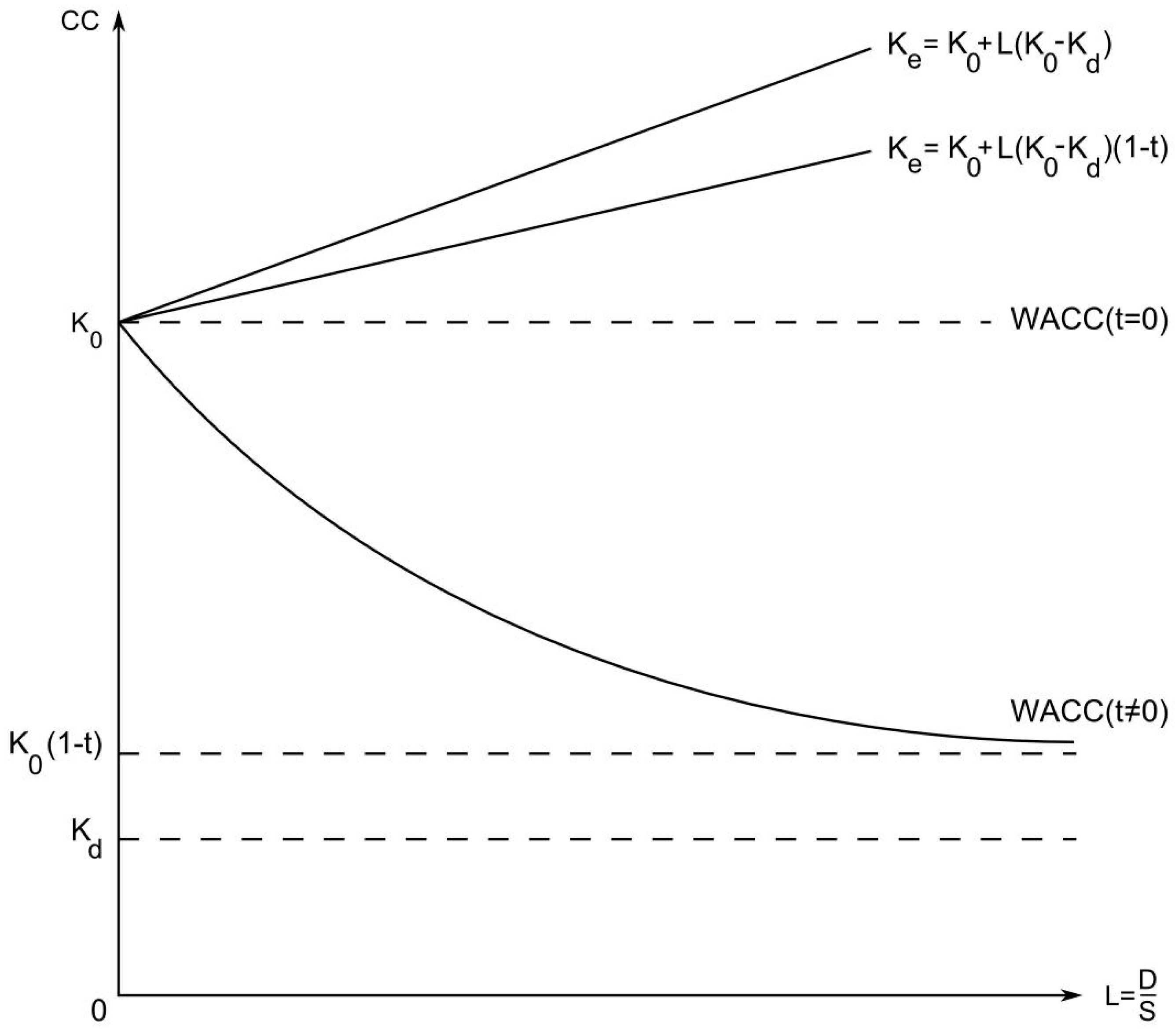
1] Modigliani and Miller (MM) under a lot of assumptions (there are no taxes, no bankruptcy costs, no transaction costs, perfect financial markets exist with symmetry information, equivalence in borrowing costs for both companies and investors, etc.), came to the conclusions that choosing of the ratio between the debt and equity capital does not affect company value as well as capital costs (Figure 1). These conclusions were fundamentally different from the conclusions of the traditional approach.
Modigliani and Miller, under the above assumptions, have analyzed the impact of financial leverage, assuming the absence of any taxes (on corporate profit as well as individual one). They have formulated and proven two following theorems.
Without taxes, the total cost of any company is determined by the value of its EBIT (Earnings Before Interest and Taxes), discounted with fixed rate k0, corresponding to group of business risk of this company: This leads to the following expressions for WACC:
Note, that k0 here and below is the weighted average cost of capital, WACC for an unleveraged company. For a leveraged company, k0 is the equity cost (and weighted average cost of capital, WACC) at zero leverage level (L = 0).
From the first Modigliani–Miller theorem [
1], it is easy to derive an expression for the equity capital cost:
Finding from here
ke, one gets
Here,
| D | value of debt capital of the company; |
| S | value of equity capital of the company; |
| cost and fraction of debt capital of the company; |
| cost and fraction of equity capital of the company; |
WACC | financial leverage;
weighted average cost of capital. |
Thus, we come to second theorem of Modigliani–Miller theory regarding the equity cost of a leveraged company (Modigliani and Miller 1958).
The equity cost of a leveraged company (ke) could be found as k0 (the cost of equity of an unleveraged company with the same asset risk), plus premium for risk, which is equal to the product of difference (k0 − kd) and leverage level L: Formula (5) shows that equity cost of the company increases linearly with is leverage level.
2. Some Modifications of Modigliani–Miller Theory
2.1. Modigliani–Miller Theory with Taxes
In 1963 Modigliani and Miller [
2] accounted for the effect of corporate taxes and obtained the following result for the capitalization value of a leveraged company,
V:
where
V0 is the value of unleveraged company,
D is the debt value and
T is the corporate taxes on profit rate.
The value of a leveraged company is equal to the value of the unleveraged company with the same asset risk, plus the value of tax shield arising from financial leverage, which is equal to the product of corporate income tax rate (T) and the debt value (D).
The following section presents the formal derivation result for WACC and the equity capital cost (ke) of the company with consideration of corporate taxes.
2.1.1. Weighted Average Cost of Capital, WACC
The below is a very important formula for weighted average cost of capital (WACC) and is one of the main results of the Modigliani–Miller theory with taxes.
2.1.2. Equity Cost
Let us derive formula for equity cost.
On definition of the weighted average cost of capital with “tax shield”, we have:
Equating Equations (9) and (10), one gets:
and from here, for equity cost, we develop the following expression:
Therefore, we see the following theorem obtained by Modigliani and Miller in 1963 [
2]:
Equity cost of leveraged company (ke) could be found as equity cost of unleveraged company (k0) with the same business risk, plus premium for risk, the value of which is equal to the triple product of difference between the cost of capital for an unleveraged firm and cost of debt (k0 − kd), leverage level and tax corrector (1 … T).
It should be noted that Formula (12) is different from Formula (5) without tax only by the multiplier (1 – T), suggesting the tax benefit of debt will lower the cost of equity as well.
Analysis of Formulas (5), (9) and (12) leads to the following conclusions. When leverage grows:
The value of company increases.
The weighted average cost of capital WACC decreases from k0 (at ) up to (at ) (when the company is funded solely by borrowed funds).
Equity cost increases linearly from k0 (at ) up to (at ).
Within their theory, Modigliani and Miller (1963) came to the following conclusions regarding the growth of financial leverage (
Figure 1).
2.2. Taking into Account Market Risk: Hamada Model
In 1969 Hamada [
9] united CAPM (Capital Asset Pricing Model) and Modigliani–Miller theory with taxes. For the equity cost of a leveraged company, the following formula has been derived, which includes financial and business risk of company:
here
bU is the CAPM
βeta of the unleveraged company with the same asset risk as the leveraged company under consideration. Formula (13) represents the cost of equity (
ke) for a leveraged firm as a sum of three components: risk-free rate (
kF), risk premium for business/asset risk
and risk premium for financial risk
.
If the company does not have borrowing (D = 0), the financial risk factor will be equal to zero (the third term is drawn to zero), and equity holder will only require the premium for business/asset risk.
2.3. The Account of Corporate and Individual Taxes (Miller Model)
In their second article, Modigliani and Miller (1963) [
2] only considered corporate taxes benefit of debt but did not take into account the effect of individual investors’ income taxes.
Merton Miller [
10], in 1977, developed such a model, showing the influence of financial leverage on the capitalization of the company when the effects of both corporate and individual taxes are accounted for, i.e., there is double taxation on corporate earnings. We will use the following definitions:
TC—corporate taxes rate and
TS—a weighted average value of effective taxes rates on dividends and capital gains on shares. With the same other assumptions that have been made for Modigliani–Miller models previously, the unleveraged company value can be determined as follows:
A term accounts for the individual taxes. The numerator in (1) indicates which part of the operating company’s profit remains in the possession of the investors, after the company earnings are taxed twice: by corporate taxes and individual taxes. Since individual taxes reduce investors’ residual income, it also reduces the overall assessment of the unleveraged company value.
2.4. Brusov–Filatova–Orekhova (BFO) Theory
One of the most serious limitations of the Modigliani–Miller theory is the suggestion about the perpetuity of the companies. In 2008, Brusov–Filatova–Orekhova [
4] considered this limitation and showed that accounting for the finite lifetime length (or arbitrary age
n) of the company leads to significant changes of all Modigliani–Miller results [
1,
2,
3]: capitalization of the company V is changed, as well as the equity cost,
ke, and the weighted average cost of capital, WACC, in the presence of corporative taxes. Moreover, a number of new findings for corporate finance, in the Brusov–Filatova–Orekhova theory [
4], are absent in Modigliani–Miller theory.
The formula for weighted average cost of capital (WACC) for the company with arbitrary age
n, as derived by Brusov–Filatova–Orekhova, has the following form [
4]:
Here,
is the debt share; k0 is the cost of capital for an unleveraged firm with the same asset risk; kd the cost of debt; T denotes the corporate taxes rate; and n stands for the firm’s lifetime length (age).
A perpetuity (Modigliani–Miller) limit could be easily obtained from (14), substituting .
A lot of meaningful effects have been discovered within the BFO theory: these effects are absent within MM theory. BFO theory has challenged some main existing principles of financial management: among them the trade-off theory, which has been prevailing for many decades and established the foundation to claim the existence of an optimal capital structure for firms. However, BFO theory has proven the bankruptcy of trade-off theory [
4].
2.5. The General WACC Formula
A more general formula for WACC, the famous Modigliani–Miller theory (MM) has been derived and discussed by a few authors in 2006–2007 [
11,
12,
13,
14]. It takes the following form (Equation (18) in [
11]).
where
k0 is the required return on unleveraged company,
kd is the required return on its debt,
kTS is the expected return on the tax shield and
t is the corporate taxes rate.
This formula is derived from the definition of the weighted average cost of capital and the balance sheet identity (for a similar presentation, see [
13]). At any point in time, it should therefore be verified, regardless of whether returns are annually or continuously compounded.
Practical applicability of Equation (15) (while it is fairly general) requires additional conditions. Indeed, when the WACC is constant over time, the value of a leveraged company can be computed by discounting with the WACC of the unlevered free cash–flows. Therefore, it is interesting to consider the special cases when WACC is constant. The resulting formulas can also be found in textbooks [
15,
16].
It was assumed by Modigliani and Miller in 1963 [
2] that the debt value D is constant. As the expected after-tax cash-flow of the unleveraged company is fixed, V
0 is also constant. By this assumption, k
TS = k
D and the value of the tax shield is TS = tD. Therefore, the capitalization of the leveraged company V is a constant and the general WACC Formula (15) simplifies to a constant WACC:
However, our opinion is that “classical” Modigliani–Miller (MM) theory, which suggests that the expected returns on the debt kd and the tax shield kTS are equals (because both of them have debt nature), is much more reasonable and in our paper we modify the “classical” Modigliani–Miller (MM) theory, which is still widely used in practice.
2.6. Trade–Off Theory
The world-famous trade-off theory has been considered the cornerstone in the solution of the problem of optimal capital structure for a company for many decades and is still used today for decision analysis on capital structure. Below we give two examples.
Frank, M., & Goyal, V., in their 2009 paper [
17], “examines the relative importance of many factors in the capital structure decisions of publicly traded American firms from 1950 to 2003. The most reliable factors for explaining market leverage are: median industry leverage (+ effect on leverage), market-to-book assets ratio (−), tangibility (+), profits (−), log of assets (+), and expected inflation (+)”. In addition, the authors have found that “dividend-paying firms tend to have lower leverage. When considering book leverage, somewhat similar effects are found. However, for book leverage, the impact of firm size, the market-to-book ratio, and the effect of inflation are not reliable”. The empirical evidence seems to be reasonably consistent with some versions of the trade-off theory of capital structure.
Serrasqueiro, Z., & Caetano, A., in 2015 [
18], analyzed “to what extent decisions on the capital structure of small and medium–sized enterprises (SMEs) are closer to the assumptions of trade–off theory or to the assumptions of hierarchy theory. They used a sample of small and medium–sized enterprises located in the Portuguese hinterland, using dynamic LSDVC as the valuation method, and the empirical evidence suggests that the most profitable and oldest SMEs are less leveraged, confirming Pecking Order Theory ‘s forecasts. Larger SMEs are leveraging more borrowing, confirming the predictions of trade–off theory and hierarchy theory. In addition, SMEs are significantly adjusting their current debt levels towards the optimal debt ratio, which is consistent with the predictions of the compromise theory. It was concluded that theories of compromise and hierarchy are not mutually exclusive in explaining capital structure decisions of small and medium–sized enterprises”.
However, the bankruptcy of trade-off theory has been proven by Brusov et al. in 2013 [
4]. They have shown that risky debt financing (and growing credit rate near the bankruptcy) in contrast to waiting results does not lead to growing of weighted average cost of capital, WACC, which still decreases with leverage. This means the absence of minimum in the dependence of WACC on leverage level as well as the absence of maximum in the dependence of company capitalization on leverage. Thus, the well-known trade-off theory lacks an optimal capital structure. The explanation for this fact was made by Brusov et al. in 2013 [
4] by analyzing the dependence of the cost of equity capital on the leverage level on the assumption that debt capital is risky.
Modigliani–Miller have considered tax shields from the interest on debt can increase the value of companies. In 1980, De Angelo and Masulis [
19] moved further in the theoretical examination of tax shields. They have noted that there are tax deductibles for companies other than debt to reduce their corporate tax burden and debt and non-debt tax shields should be accounted for. Depreciation, investment tax credits, or net-loss carry forwards could represents examples of such kind of non-debt tax shields. The first to test for these tax effects (suggested by DeAngelo and Masulis in 1980 [
19]) has been carried out by Bradley, Jarrell and Kim in 1984 [
20]. In contrast to the prediction in De Angelo and Masulis [
19], by regressing company-specific debt-to-value ratios on non-debt tax shields, they have shown that debt is positively related to non-debt tax shields as measured by depreciation and investment tax credits. Titman and Wessels in 1988 [
18] found that “their results do not provide support for an effect on debt ratios arising from non-debt tax shields…”. It was pointed out in 2003 by Graham [
21], if a company invests heavily and uses debt financing to invest, a positive relation between such proxies for non-debt tax shield and debt may result. A mechanical positive relation of this type overwhelms and renders any substitution effects between debt and non-debt tax shields.
The original theory by Nobel Prize Winners Modigliani and Miller [
1,
2,
3] has been modified by many authors and above we shortly discussed some of them. In next paragraph we will generalize for the first time the Modigliani–Miller theory for the case of variable profit.
4. Results and Discussion
In this section we study numerically (within Microsoft Excel) the dependence of the weighted average cost of capital, WACC, discount rate, i, company value, V, and equity cost, ke, on leverage level L in the Generalized Modigliani–Miller theory (GMM theory) at two values of equity cost k0 (0.2 and 0.3) and different values of growth rate, g. The obtained results are discussed.
4.1. Dependence of WACC on Leverage Level L in Generalized Modigliani–Miller Theory (GMM Theory) at k0 = 0.2 and Different Values of g (0.4; 0.3; 0.2; 0.0; −0.2; −0.3; −0.4)
We study first the dependence of the weighted average cost of capital, WACC, on leverage level L in Generalized Modigliani–Miller theory (GMM theory) at k0 = 0.2 and different values of g (0.4; 0.3; 0.2; 0.0; −0.2; −0.3; −0.4).
From
Figure 2 it is seen that all curves WACC(L) for different g start from one point k
0, in this case from point (0; 0.2). They decrease with leverage level L at g < 0.2 (at g = 0; ±0.2; −0.3; −0.4) and increase at g > 0.2 (at g = 0.3; 0.4). The curves WACC(L) increase with growth rate, g. Note, that cut–off value of g, which separate increasing curves WACC(L) from decreasing ones is equal to k
0 = 0.2, and WACC is constant at g = k
0 and equal to k
0. Below we check this observation at different value of k
0 (k
0 = 0.3).
4.2. Dependence of the Weighted Average Cost of Capital WACC on Leverage Level L in Generalized Modigliani–Miller Theory (GMM Theory) at k0 = 0.3 and Different Values of g
Let us study the dependence of WACC on leverage level L in Generalized Modigliani–Miller theory (GMM theory) at k0 = 0.3 and different values of g.
From
Figure 3 it is seen that all curves WACC(L) for different g start from one point, k
0, in this case from (0; 0.3). They decrease with L at g < 0.3 (at g = 0; ±0.2; ±0.3; −0.4) and increase at g > 0.3 (at g = 0.4). Note, that thr cut-off value of g, which separate increasing curves WACC(L) from decreasing ones as in above case is equal to k
0 (k
0 = 0.3), and WACC is constant at g = k
0 and equal to k
0. Therefore, our observation that this conclusion is valid at different value of k
0 is right.
From
Figure 2 and
Figure 3 it is seen that all curves WACC(L) for different g start from one point, k
0. They decrease with L at g < k
0 and increase at g > k
0. It turns out that WACC grows with g, while, as we will see below, real discount rates WACC–g and k
0–g decrease with g. This leads to increase of company capitalization with g: V = CF/WACC–g.
4.3. Dependence of Discount Rate i on Leverage Level L in Generalized Modigliani–Miller Theory (GMM Theory) at k0 = 0.2 and Different Values of g
Discount rate for the leverage company change from the weighted average cost of capital, WACC, to WACC–g (where g is growth rate), for a financially independent company from k0 to k0–g. This means that WACC and k0 are no longer the discount rates as it takes place in case of the classical Modigliani–Miller theory with constant profit. Below we study the dependence of discount rate i on leverage level L in Generalized Modigliani–Miller theory (GMM theory) at two values of k0 (0.2; 0.3) and different values of g (−0.4; −0.3; −0.2; 0.0; 0.1; 0.15; 0.2; 0.3; 0.4). Let us start from k0 = 0.2.
From
Figure 4 it is seen that discount rate i decreases with leverage level L at growth values g < k
0 (at g = 0; 0.1; 0.15; ±0.2; −0.3; −0.4). Discount rate i in contrast to WACC decreases with g: this provides the increase of company value V with g.
At g > k
0 discount rate i increases with L, but being negative it is not shown in
Figure 4.
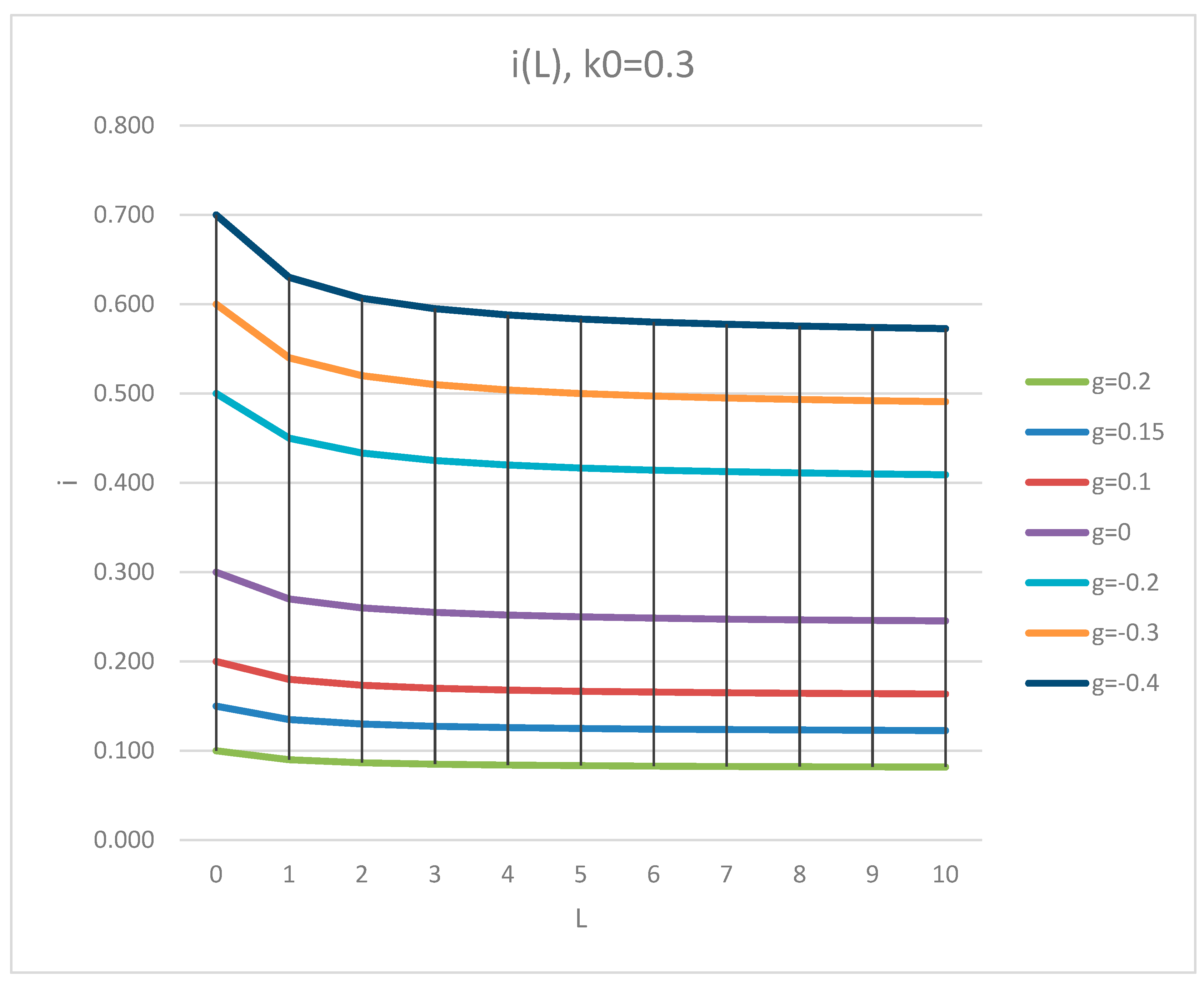
4.4. Dependence of Discount Rate i on Leverage Level L in Generalized Modigliani–Miller Theory (GMM Theory) at k0 = 0.3 and Different Values of g
Let us study the dependence of discount rate i on leverage level L in Generalized Modigliani–Miller theory (GMM theory) at k0 = 0.3 and different values of g.
From
Figure 5 it is seen that discount rate i decreases with leverage level L at growth values at g < k
0 (at g = 0; 0.1; 0.15; ±0.2; −0.3; −0.4). Discount rate i in opposite to WACC decreases with g: this provides the increase of company value V with g.
At g > k
0 discount rate i increases with L, but being negative it is not shown in
Figure 5.
From
Figure 4 and
Figure 5 it is seen that for k
0 = 0.2 and 0.3 discount rate i decreases with g: this provides the increase of company value V with g. Discount rate i decreases with L at g < k
0 (at g = 0; 0.1; 0.15; ±0.2; −0.3; −0.4). At g > k
0 discount rate i increases with L, but being negative it is not shown in
Figure 4 and
Figure 5.
4.5. Dependence of Company Value V on Leverage Level L in Generalized Modigliani–Miller Theory (GMM Theory) at k0 = 0.2 and Different Values of g
Let us study the dependence of company value V on leverage level L in Generalized Modigliani–Miller theory (GMM theory) at k0 = 0.2 and different values of g.
From
Figure 6. it is seen, that at k
0 = 0.2 and g = 0; 0.1; 0.15; −0.2; −0.3; −0.4 the company value V at fixed growth rate g increases with leverage level L in Generalized Modigliani–Miller theory (GMM theory). The company value V also increases with growth rate g.
4.6. Dependence of Company Value V on Leverage Level L in Generalized Modigliani–Miller Theory (GMM Theory) at k0 = 0.3 and Different Values of g
Let us study the dependence of company value V on leverage level L in Generalized Modigliani–Miller theory (GMM theory) at k0 = 0.3 and different values of g.
From
Figure 7 it is seen, that at k
0 = 0.3 and g = 0; 0.1; 0.15; −0.2; −0.3; −0.4 the company value V at fixed growth rate g increases with leverage level L in Generalized Modigliani–Miller theory (GMM theory). The company value V as well increases with growth rate g.
From
Figure 6 and
Figure 7 it is seen, that at two values of k
0 (0.2; 0.3) and g = 0; 0.1; 0.15; −0.2; −0.3; −0.4 the company value V at fixed growth rate g increases with leverage level L in Generalized Modigliani–Miller theory (GMM theory). The company value V as well increases with growth rate g.
We should note that in case of growing rate g equals to equity cost (at L = 0) k0, the company value V becomes infinite. This is the limitation of the perpetuity Modigliani–Miller theory. As one can see in our future publications where we will consider the generalization of BFO theory for the case of variable profit such kind of restriction is absent for companies of finite ages.
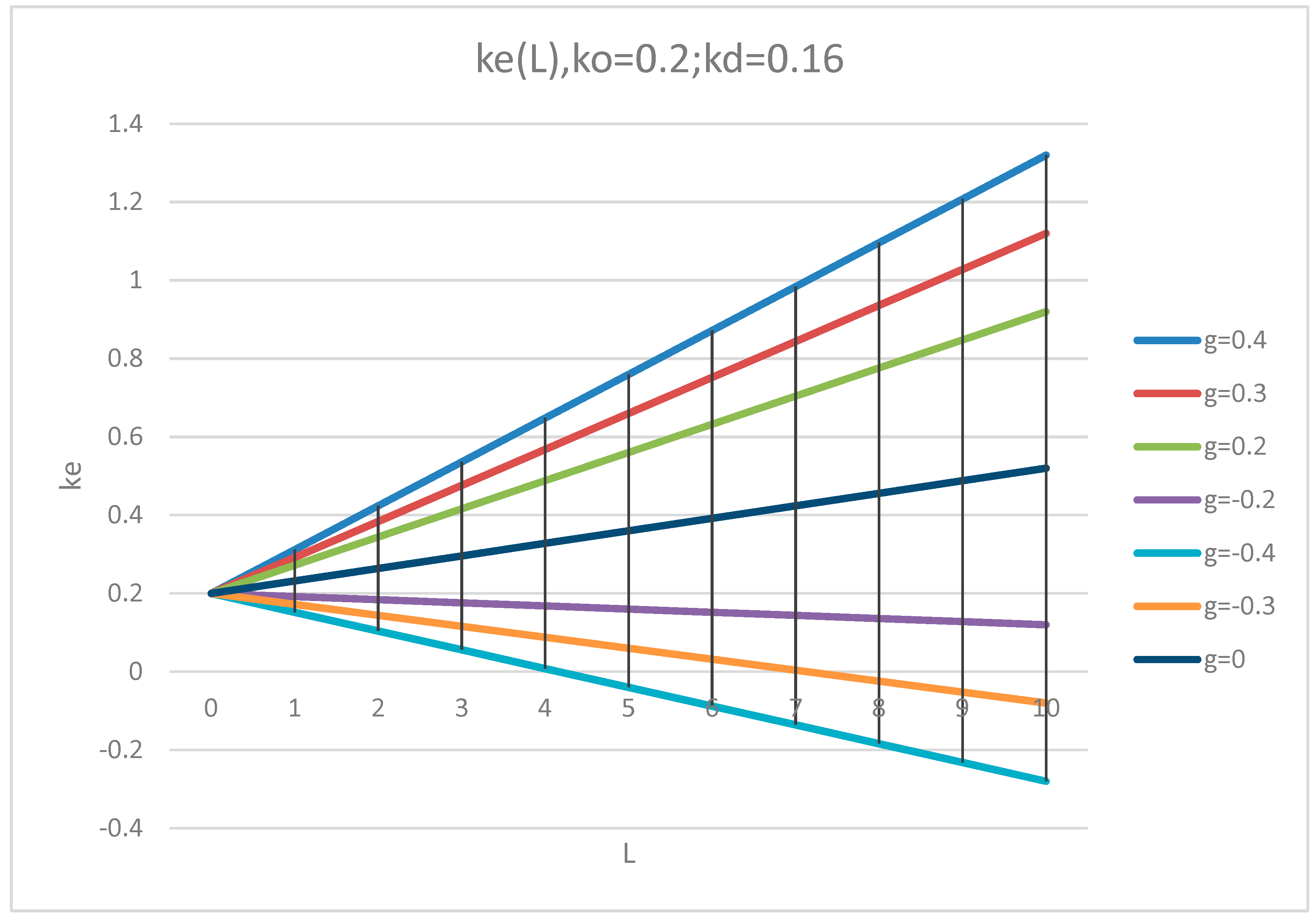
4.7. Dependence of Equity Cost ke on Leverage Level L in Generalized Modigliani–Miller Theory (GMM Theory) at k0 = 0.2 and Different Values of g (0; ±0.2; ±0.3; ±0.4)
The economically justified value of dividends is equal to equity cost. Thus, knowing the dependence of equity cost of company on leverage level L, on growth rate g is very important, because it could impact the dividend policy of the company and help to company management to develop reasonable dividend policy.
Below we study the dependence of equity cost ke on leverage level L in Generalized Modigliani–Miller theory (GMM theory) at k0 = 0.2 and different values of g (0; ±0.2; ±0.3; ±0.4).
We have investigated the dependence of equity cost k
e on leverage level L in the Generalized Modigliani–Miller theory (GMM theory) at k
0 = 0.2 and g = 0; ±0.2; ±0.3; ±0.4. From
Figure 8 it is seen that the equity cost, ke, which linearly grows with leverage level L increases with g: the tilt angle ke(L) grows with g. It is interesting, that at k
0 = 0.2; k
d = 0.16 and at g* = −0.16 in accordance with formula
the equity cost ke turns out to be equal to k
0 and does not change with leverage level L.
This should change the dividend policy of the company, because the economically justified value of dividends is equal to equity cost.
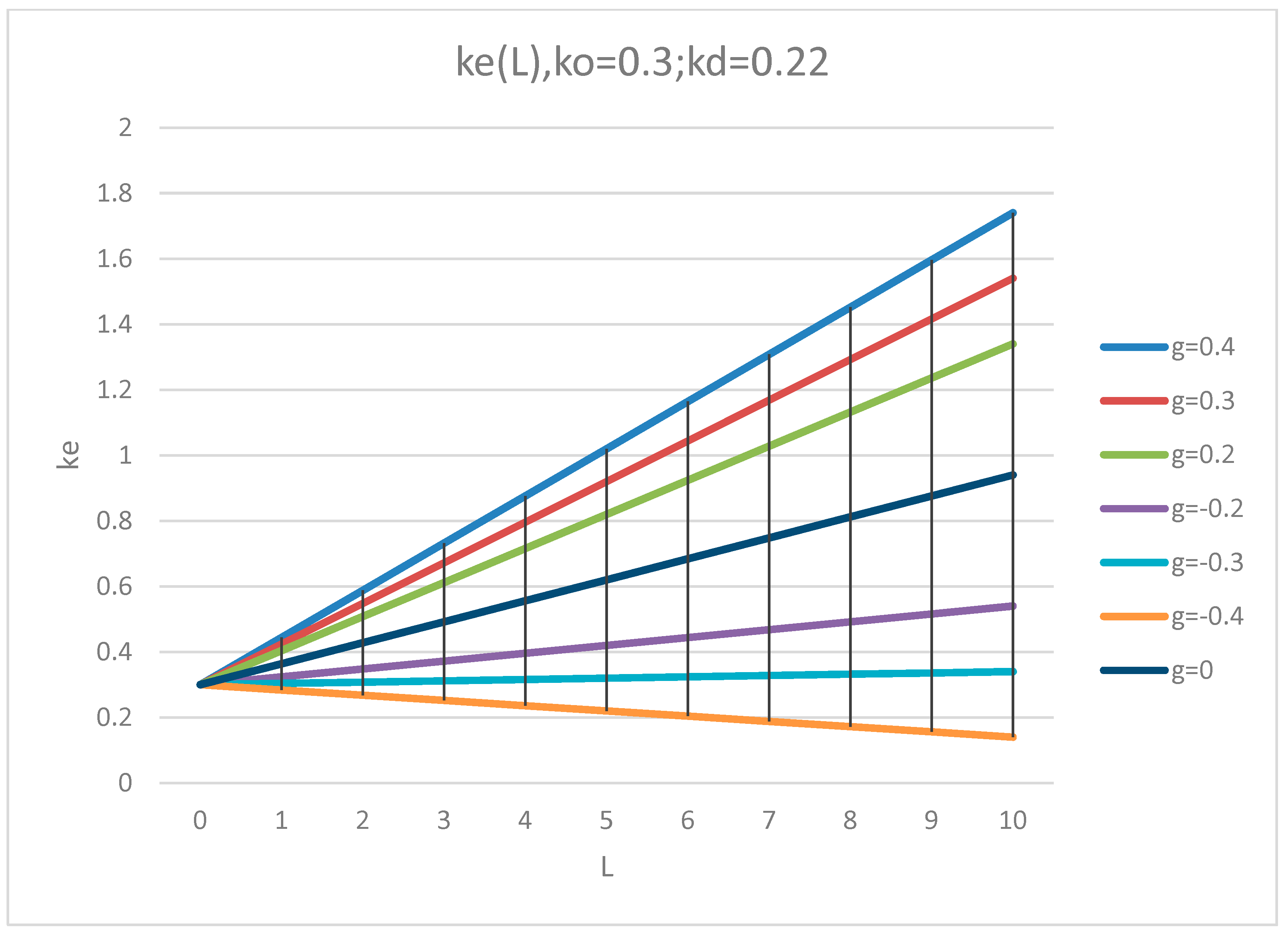
4.8. Dependence of Equity Cost ke on Leverage Level L in Generalized Modigliani–Miller Theory (GMM Theory) at k0 = 0.3 and Different Values of g
Presented below is the dependence of equity cost ke on leverage level L in the Generalized Modigliani–Miller theory (GMM theory) at k0 = 0.3 and different values of g (0; ±0.2; ±0.3; ±0.4).
We have investigated the dependence of equity cost k
e on leverage level L in the Generalized Modigliani–Miller theory (GMM theory) at k
0 = 0.3 and g = 0; ±0.2; ±0.3; ±0.4. From
Figure 9 it is seen that the equity cost, ke, which linearly grows with leverage level increases with g: the tilt angle ke(L) grows with g. It is interesting, that at k
0 = 0.3; k
d = 0.22 and at g* = −0.32 in accordance with Formula (43) the equity cost ke turns out to be equal to k
0 and does not change with leverage level L.
Here, we have investigated the dependence of equity cost ke on leverage level L in Generalized Modigliani–Miller theory (GMM theory) at two values of k0 (0.2 and 0.3) and different values of g. The equity cost, ke, which linearly grows with leverage level increases with g: the tilt angle ke(L) grows with g. This should change the dividend policy of the company, because the economically justified value of dividends is equal to equity cost.
It is interesting, that at k0 = 0.2; kd = 0.16 and at g* = −0.16 and at k0 = 0.3; kd = 0.22 and at g* = −0.32 in accordance with Formula (43) the equity cost ke turns out to be equal to k0 and does not change with leverage level L.
The qualitatively new effect in corporate finance has been discovered: at rate g < g* the slope of the curve ke(L) turns out to be negative. This effect, which is absent in classical Modigliani–Miller theory, could significantly alter the principles of the company’s dividend policy.
The last effect is similar to the qualitatively new effect in corporate finance, which has been discovered by Brusov–Filatova–Orekhova within the BFO theory [
4]: abnormal dependence of equity cost ke on leverage level at tax on profit rate T, which exceed some rate value T*: this discovery also significantly alters the principles of the company’s dividend policy.
5. Conclusions
The main purpose of the current study is to generalize the Modigliani–Miller theory by taking into account one of the most important conditions of companies real functioning: variable profit. We use analytical and numerical methods: we derive all main formulas of the Generalized Modigliani–Miller theory theoretically and then use them to obtain all the main financial indicators of company and their dependences on different parameters by MS Excel. The generalized Modigliani–Miller theory significantly extends its application in practice, especially in business valuation, in ratings and in other areas of economy and finance. We consider the case of growing profit as well as decreasing of profit and show, that all the statements by Modigliani and Miller change significantly.
Within the new Generalized Modigliani–Miller theory (GMM theory), we study the dependence of the weighted average cost of capital, WACC, the cost of equity, ke, the discount rate i and the capitalization of the company, V, on leverage level L at different values of growth rate g and obtained the following results:
Discount rate for leverage company changes from the weighted average cost of capital, WACC, to WACC–g (where g is growing rate), for a financially independent company from k0 to k0–g. This means that WACC and k0 are no longer the discount rates as it takes place in case of classical Modigliani–Miller theory with constant profit.
All curves WACC(L) for different g start from one point, k0. They decrease with L at g < k0 and increase at g > k0. It turns out that WACC grows with g, while real discount rates WACC–g and k0–g decrease with g. This leads to increase of company capitalization with g: V = CF/WACC–g.
We have investigated the dependence of equity cost ke on leverage level L in the Generalized Modigliani–Miller theory (GMM theory) at two values of k0 (0.2 and 0.3) and different values of g. The equity cost, ke, which linearly grows with leverage level L increases with g: the tilt angle ke(L) grows with g. This should change the dividend policy of the company, because the economically justified value of dividends is equal to equity cost.
It is interesting, that at k0 = 0.2; kd = 0.16 and at g* = −0.16 and at k0 = 0.3; kd = 0.22 and at g* = −0.32 in accordance with Formula (43) the equity cost ke turns out to be equal to k0 and does not change with leverage level L.
A new qualitative finding related to corporate finance has been discovered in this study: at rate g < g* the slope of the curve ke(L) turns out to be negative. This effect, which is absent in the classical Modigliani–Miller theory, could significantly alter the principles of the company’s dividend policy. Rating methodology should take into account the company’s dividend policy [
5], thus such results obtained could change the credit rating of an issuer.
The last effect found in this study is similar to the qualitatively new effect in corporate finance, discussed above, which has been discovered by Brusov–Filatova–Orekhova within BFO theory: abnormal dependence of equity cost on leverage level when corporate taxes rate T exceeds some rate value T*; this discovery also significantly alters the principles of the company’s dividend policy.
Thus, within the new Generalized Modigliani–Miller theory, a lot of significant implications are obtained, allowing us to develop new approach to financial policy and financial strategy of the company.
Note that the limitations of the Generalized Modigliani–Miller theory are similar to the limitations of the classical Modigliani–Miller theory and are connected with the numerous assumptions of classical Modigliani–Miller theory [
1,
2,
3]. Therefore, the direction of future research is clear: we will consider the generalization of BFO theory, which describes the companies of arbitrary age, for the case of variable profit. The limitations of the Generalized Modigliani–Miller theory will be absent in the generalized BFO theory, which is valid for companies of an arbitrary age.
The Generalized Modigliani–Miller theory could and should be used in corporate finance and corporate management, in investments, business valuation, taxation, ratings, etc., for more correct assessments and more qualified management decisions.
Authors planning further development of the Modigliani–Miller theory should account for practical conditions of business and its application in all mentioned above areas. In particular, more frequent payments of tax of profit will be considered, combination of this case with advance payments of tax of profit, modification of BFO theory (which is valid for the companies of arbitrary ages) for the case of variable profit.


 ,
, 


