Analysis of Stochastic Generation and Shifts of Phantom Attractors in a Climate–Vegetation Dynamical Model

Abstract

A problem of the noise-induced generation and shifts of phantom attractors in nonlinear dynamical systems is considered. On the basis of the model describing interaction of the climate and vegetation we study the probabilistic mechanisms of noise-induced systematic shifts in global temperature both upward (“warming”) and downward (“freezing”). These shifts are associated with changes in the area of Earth covered by vegetation. The mathematical study of these noise-induced phenomena is performed within the framework of the stochastic theory of phantom attractors in slow-fast systems. We give a theoretical description of stochastic generation and shifts of phantom attractors based on the method of freezing a slow variable and averaging a fast one. The probabilistic mechanisms of oppositely directed shifts caused by additive and multiplicative noise are discussed.

1. Introduction

Mathematical modeling and analysis of complex interrelations of climate and vegetation has attracted the attention of many researchers [1,2,3,4,5]. In processes of identifying fundamental laws of these interrelations, simple conceptual models play a key role. Here, one of the well known and most effectively used is the two-dimensional model proposed by Rombouts and Ghil [6]. Because of strong nonlinearity of climate–vegetation feedbacks, this model exhibits bistability with coexisting equilibria and limit cycles. Complex stochastic effects in this system were studied numerically in [7,8].

In nonlinear systems, the inevitably present random noise can dramatically change behavior scenarios [9,10,11], and cause stochastic bifurcations [12,13], noise-induced transitions [14,15], excitement [16,17], noise-induced chaos [18], etc. Recently, a new stochastic phenomenon of the localization of random states of the system away from its attractors was discovered. This phenomenon called “phantom attractor” has been observed in models of enzymatic reactions, neurodynamics [19], population dynamics [20], geophysics [21]. Phantom attractors in the stochastically forced climate–vegetation model were found by direct numerical simulation [8]. The present paper aims to elaborate methods of theoretical analysis of this phenomena for different types of stochastic forcing.

In Section 2, we discuss peculiarities of the deterministic climate–vegetation model under consideration and present results of the bifurcation analysis. Here, coexistence of attractors corresponding to “warm” and “cold” states of the system is shown.

In Section 3, we present results of numerical simulation of solutions for the stochastically forced climate–vegetation model. Here, we show that additive and multiplicative noises cause opposite effects in the global temperature, and associate these effects with the phenomenon of the phantom attractor.

Section 4 aims to give the theoretical justification for the phantom attractor. This mathematical theory is based on the method of freezing and averaging used in the analysis of slow-fast systems [22,23,24].

Here we study in detail the cases of additive and multiplicative noise, as well as the general case of their combined effect. All theoretical conclusions are verified by results of direct numerical simulation.

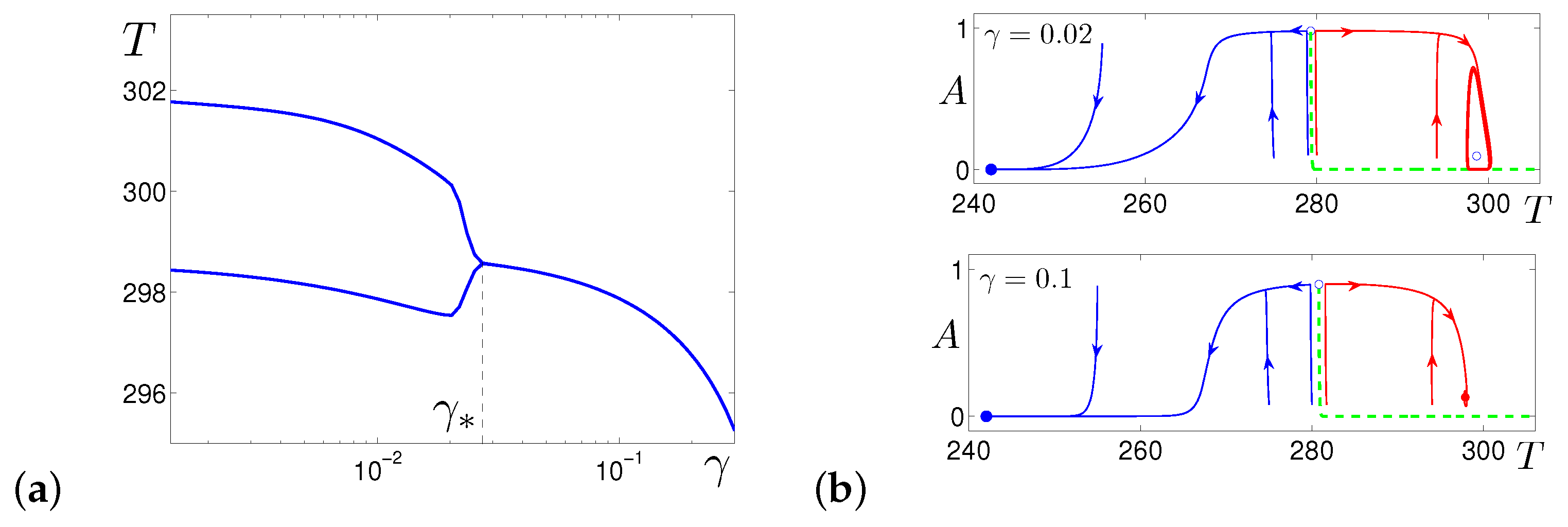
2. Deterministic Model

To study a role of stochastic disturbances in the climate–vegetation interaction, as a deterministic skeleton, we will consider the mathematical model suggested in [6]

$$\begin{array}{c}{\displaystyle C_T\frac{dT}{dt}=(1-\alpha (T,A))Q_0-R_o\left(T\right),}\hfill \\ {\displaystyle \frac{dA}{dt}=\beta \left(T\right)A(1-A)-\gamma A.}\hfill \end{array}$$

(1)

Here, the variable T denotes global average temperature, while A denotes the fraction of land that is covered by vegetation. Parameters $C_T$ and $Q_0$ represent the heat capacity and the incoming solar energy, respectively. In the system (1), the function

$$\alpha (T,A)=(1-q){\alpha }_o\left(T\right)+q({\alpha }_{v}A+{\alpha }_g(1-A))$$

determines the total surface albedo. Here,

$${\alpha }_o\left(T\right)=\left\{\begin{array}{cc}{\alpha }_{max},\hfill & T\le T_{\alpha ,l},\hfill \\ {\alpha }_{max}+\frac{{\alpha }_{min}-{\alpha }_{max}}{T-T_{\alpha ,l}},\hfill & T_{\alpha ,l}<T\le T_{\alpha ,u},\hfill \\ {\alpha }_{min},\hfill & T>T_{\alpha ,u}.\hfill \end{array}\right.$$

The function

$$R_o\left(T\right)=B_0+B_1(T-T_{opt})$$

is the flux of energy leaving the planet’s surface, and $T_{opt}$ stands for the temperature which is optimal for the evolution of vegetation. This temperature $T_{opt}$ is also present in the function

$$\beta \left(T\right)=max\{0,1-k{(T-T_{opt})}^2\}$$

which describes the growth rate of vegetation [6]. In the system (1), the parameter $\gamma$ is the mean death rate of the global vegetation A.

In the present paper, we consider the system behavior in dependence on the biological parameter $\gamma$ and fix all geophysical parameters following [6]: $C_T=500$ W yr K${}^{-1}$ m${}^{-2}$, $Q_0=342.5$ W m${}^{-2}$, $q=0.3$, ${\alpha }_v=0.1$, ${\alpha }_g=0.4$, ${\alpha }_{\max }=0.85$, ${\alpha }_{\min }=0.25$, $T_{\alpha ,\ell }=263$ K, $T_{\alpha ,u}=300$ K, $B_0=200$ W m${}^{-2}$, $B_1=2.5$ W K${}^{-1}$ m${}^{-2}$, $T_{\mathrm{opt}}=283$ K, and $k=0.004$ yr${}^{-1}$ K${}^{-2}$.

A key feature of deterministic dynamics of system (1) is its bistability. For any $\gamma$, this system has the stable equilibrium ${\overline{T}}_0=242,{\overline{A}}_0=0$. This equilibrium corresponds to the “cold” state (snowball) without any vegetation. Another regime corresponding to the “warm” state can be observed in two variants: stable equilibrium or stable cycle. The point ${\gamma }_{\ast }\approx 0.0257$ of the Andronov–Hopf bifurcation separates these two regimes. For any $\gamma$, the system (1) also possesses the saddle point, and the stable manifold of this point detaches basins of attraction of “cold” and “warm” regimes. In Figure 1a, we show extrema of T-coordinates of “warm” attractors: cycles for $\gamma <{\gamma }_{\ast }$ and equilibria for $\gamma >{\gamma }_{\ast }$.

In Figure 1b, phase portraits for two values of $\gamma$ are demonstrated. Here, trajectories tending to the “cold” state are plotted by blue, and trajectories in the basin of the “warm” attractor are shown by red. The separatrix between their basins is plotted by green dashed line.

3. Stochastic Model

Consider the stochastically forced model (1)

$${\displaystyle C_T\frac{dT}{dt}=(1-\alpha (T,A))Q_0-R_o\left(T\right),}$$

(2)

$${\displaystyle \frac{dA}{dt}=\beta \left(T\right)A(1-A)-\gamma A+\epsilon ({\sigma }_{1}A{\xi }_1\left(t\right)+{\sigma }_2{\xi }_2\left(t\right)).}$$

(3)

Here, ${\xi }_{1,2}\left(t\right)$ are the standard uncorrelated white Gaussian noises with parameters $\langle {\xi }_{1,2}\left(t\right)\rangle =0$, $\langle {\xi }_{1,2}\left(t\right){\xi }_{1,2}(t+\tau )\rangle =\delta \left(\tau \right)$, $\langle {\xi }_1\left(t\right){\xi }_2(t+\tau )\rangle =0$. The multiplicative noise in (3) models random forcing $\epsilon {\sigma }_1{\xi }_1\left(t\right)$ in the parameter $\gamma$, and $\epsilon {\sigma }_2{\xi }_2\left(t\right)$ is the additive noise. In order to keep $A\left(t\right)\in [0,1]$ in the presence of random noise, we use the following truncation: if $A>1$ then $A=1$, and if $A<0$ then $A=0$.

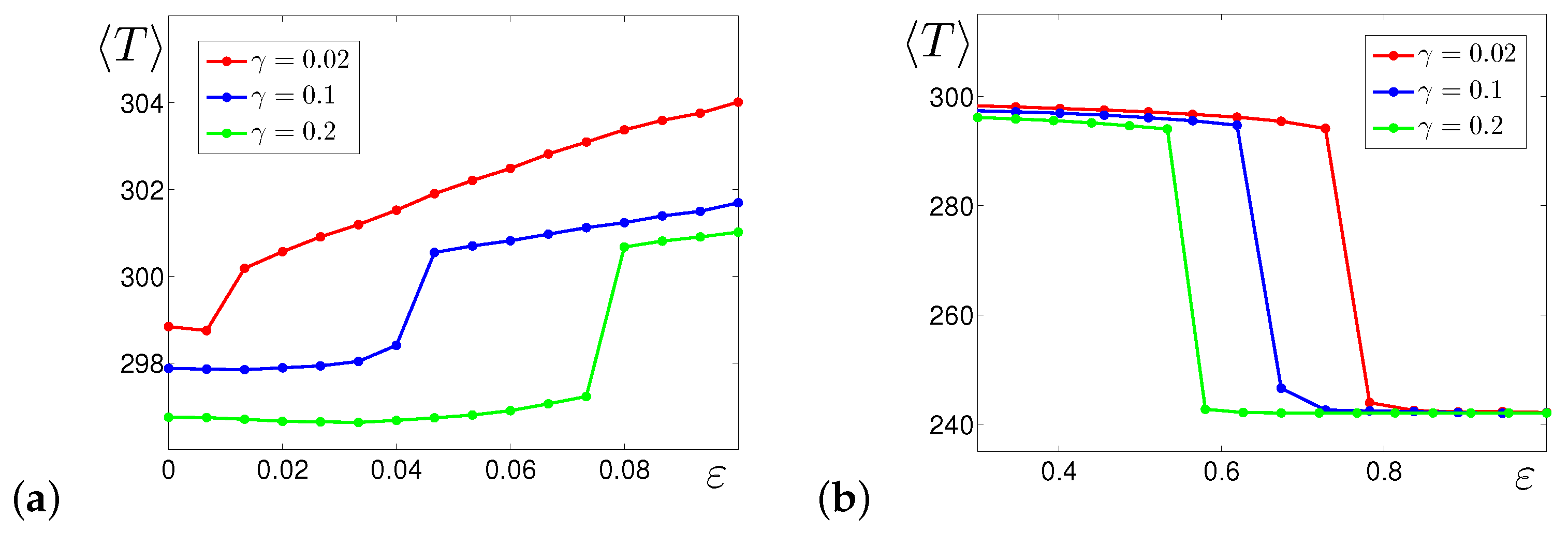
3.1. Effects of Additive Noise

Consider how additive noise changes dynamics of the climate–vegetation model. We fix ${\sigma }_1=0,{\sigma }_2=1$ and vary noise intensity $\epsilon$. First, consider $\gamma =0.1$ when the “warm” regime of deterministic system (1) is the stable equilibrium. In Figure 2a, time series of stochastic solutions starting from this equilibrium are plotted for different values of the noise intensity. For weak noise ($\epsilon =0.001$), these solutions only slightly deviate from the deterministic equilibrium. With increase in noise, along with the natural growth of dispersion, a new unexpected effect is definitely seen: random trajectories move upward from the initial stable equilibrium and stabilize near some new T-level. Note that the higher the noise intensity, the higher this T-level. This systematic shift of random solutions is clearly seen in Figure 2b where phase trajectories are shown after some transient. Note that the corresponding probabilistic distribution of random states is localized far from any deterministic attractors. To underline this peculiarity, such probabilistic distributions were called “phantom” attractors.

This effect persists over a wide range of the parameter $\gamma$. In Figure 3, time series and phase trajectories are shown for solutions starting from the deterministic limit cycle of system (1) with $\gamma =0.02$. Here, the scenario of the stochastic transformation under increasing noise has the additional initial stage: first, the amplitude of stochastic oscillations decreases (see Figure 2b for $\epsilon =0.001$), the stochastic bundle collapses into a cloud and begins to shift to the right. Onset of a such shift is accompanied by generation of intermittent oscillations in time series (see Figure 2a for $\epsilon =0.01$). With further increase in noise, one can observe a systematic shift of the “phantom” attractor to higher temperatures.

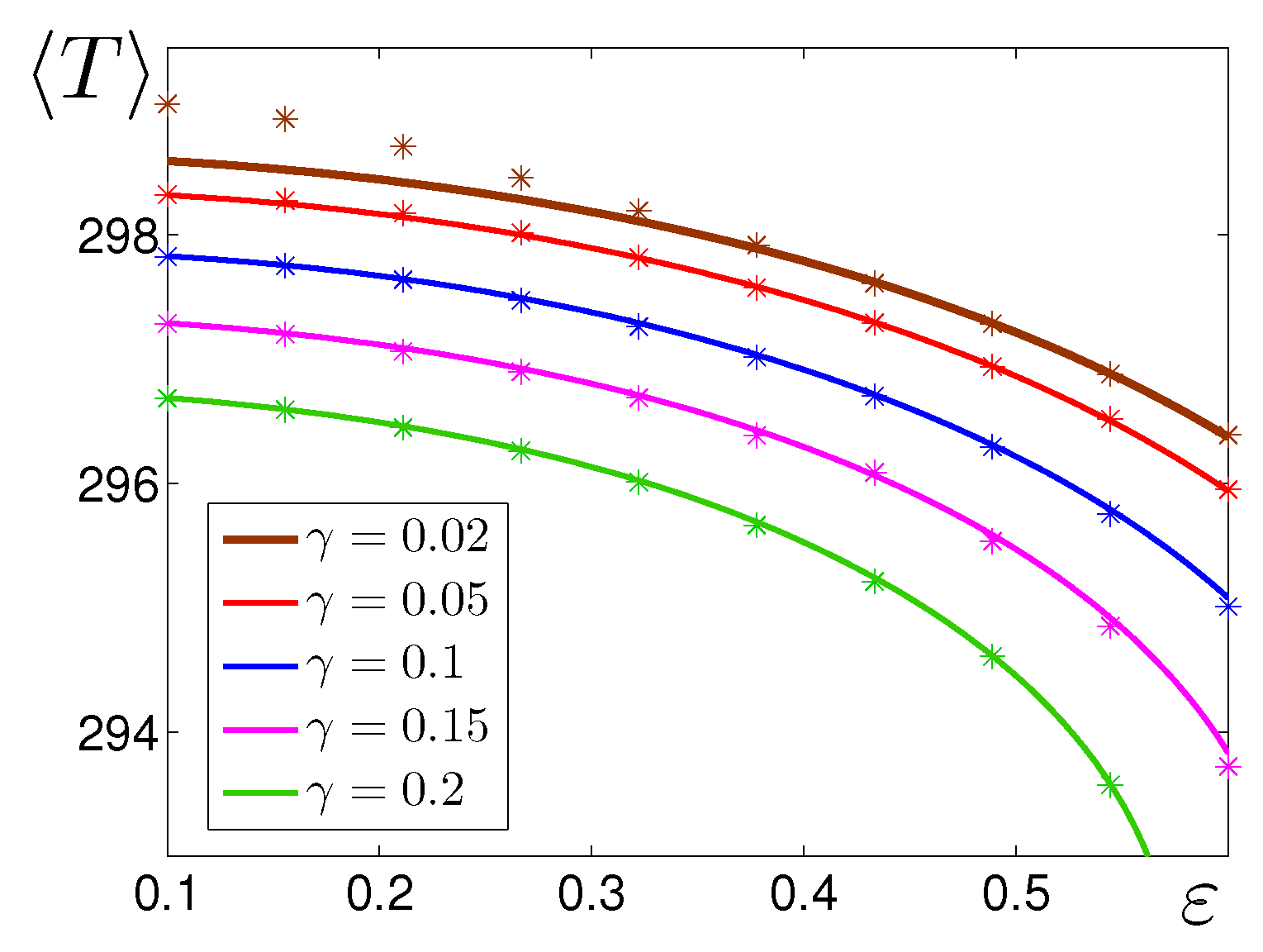
3.2. Effects of Multiplicative Noise

Consider now changes in dynamics caused by multiplicative noise. We fix ${\sigma }_1=1$, ${\sigma }_2=0$ and vary noise intensity $\epsilon$. First, consider $\gamma =0.1$ corresponding to the equilibrium “warm” regime. In Figure 4a, time series of stochastic solutions starting from the equilibrium are shown for different values of $\epsilon$. For weak noise with $\epsilon =0.05$, these solutions slightly deviate from the deterministic equilibrium. With an increase in multiplicative noise, in contrary to the case of additive noise, a systematic decrease in T-level is observed. Such a shift of the “phantom” attractor is illustrated by phase trajectories in Figure 4b. A further increase of $\epsilon$ leads to a sharp drop in the temperature to the snowball level (see Figure 4a for $\epsilon =0.7$). A similar scenario is shown in Figure 5 for $\gamma =0.02$.

A summary of the numerical simulation of systematic stochastic shifts caused by additive and multiplicative noise is concentrated in the Figure 6, where plots of mean values $\langle T\rangle$ of T-coordinates for system (2), (3) solutions in steady regime are shown for different $\gamma$ versus noise intensity $\epsilon$. Here, the following general conclusion can be done.

For additive noise (see Figure 6a), an increase of the noise intensity $\epsilon$ leads to the monotonous growth of the temperature. In this growth, one can see a narrow $\epsilon$-zone of a sharp upward jump.

For multiplicative noise (see Figure 6b), one can observe the opposite effect: an increase of $\epsilon$ leads to the monotonous decrease of the temperature T. As $\epsilon$ passes some threshold specific for each $\gamma$, a sharp drop down of the temperature to the state of snowball occurs.

As a whole, these effects can be interpreted as “additive-noise-warming” and “multiplicative-noise-freezing”. These phenomena of generation and shifts of “phantom” attractors were first found numerically and described in our early paper [8]. Now, our aim is to find an analytical explanation for all these probabilistic effects.

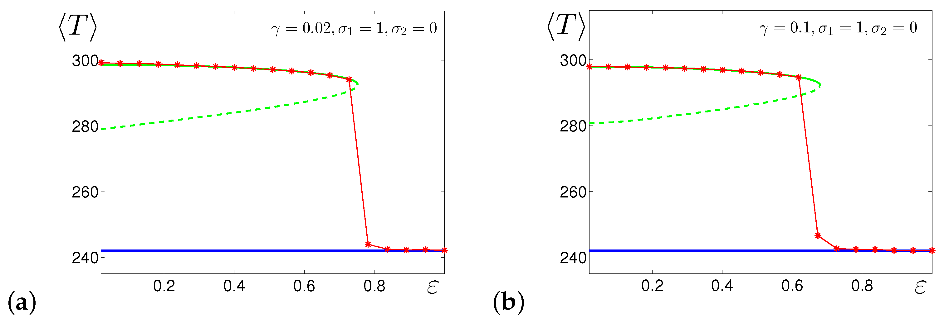
4. Method “Freeze and Average” in the Analysis of “Phantom” Attractors

For the climate–vegetation stochastic model (2), (3), in the region where “phantom” attractors are observed, the variable T changes slowly and has a small variation whereas the widely distributed variable A is fast. This means that the model (2), (3) is the slow-fast system, and the mathematical technique of freezing and averaging [22] can be applied.

At the first stage, we “freeze” the slow variable T in the stochastic system (2), (3) and consider stochastic nonlinear dynamics of the fast subsystem (3) assuming that the variable T is constant.

For any fixed T, solving the corresponding Fokker-Planck equation

$$\frac{\partial \rho }{\partial t}=-\frac{\partial }{\partial A}\left[\left(\beta \right(T\left)A\right(1-A)-\gamma A)\rho \right]+\frac{{\epsilon }^2}{2}\frac{{\partial }^2}{\partial A^2}\left[({\sigma }_1^2{A}^2+{\sigma }_2^2)\rho \right],$$

one can find an explicit representation for the stationary probability density function:

$$\rho (T,A,\epsilon )=\frac{C}{{\epsilon }^2({\sigma }_1^2{A}^2+{\sigma }_2^2)}exp\left[\frac{2}{{\epsilon }^2}\underset{0}{\overset{A}{\int }}\frac{\beta \left(T\right)s(1-s)-\gamma s}{{\sigma }_1^2{s}^2+{\sigma }_2^2}ds\right],$$

(4)

where C is the normalization constant.

Now, a behavior of the slow variable T can be described by the averaging over the fast variable A. As it follows from (2), dynamics of the mean value $m=\langle T\rangle$ is governed by the equation:

$$\dot{m}=\frac{1}{C_T}\underset{0}{\overset{1}{\int }}\left[(1-\alpha (m,A))Q_0-R_o\left(m\right)\right]\rho (m,A,\epsilon )dA.$$

(5)

So, the equilibria $\overline{m}\left(\epsilon \right)$ for the mean value m of system (5) can be found from the equation

$$\underset{0}{\overset{1}{\int }}\alpha (m,A)\rho (m,A,\epsilon )dA=1-\frac{R_o\left(m\right)}{Q_0}.$$

(6)

Note that these equilibria, both stable and unstable, are key points in the analytical explanation of noise-induced phenomena presented in Section 3.

4.1. Additive Noise

First, consider a case when the system (2), (3) is forced by the additive noise only: ${\sigma }_1=0,{\sigma }_2\ne 0.$ For this case, the Formula (4) looks as

$$\rho (T,A,\epsilon )=\frac{C}{{\epsilon }^2{\sigma }_2^2}exp\left[\frac{2}{{\epsilon }^2{\sigma }_2^2}\underset{0}{\overset{A}{\int }}\left(\beta \left(T\right)s(1-s)-\gamma s\right)ds\right]$$

After integration, the explicit representation of this stationary distribution is written as

$$\rho (T,A,\epsilon )=\frac{C}{{\epsilon }^2{\sigma }_2^2}exp\left[\frac{2}{{\epsilon }^2{\sigma }_2^2}\left((\beta \left(T\right)-\gamma )\frac{A^2}{2}-\beta \left(T\right)\frac{A^3}{3}\right)\right].$$

(7)

Using this density function $\rho (T,A,\epsilon )$, we have found stable equilibria $\overline{m}\left(\epsilon \right)$ from the Equation (6) for different values of the parameter $\gamma$. Plots of these functions, as theoretical estimations of mean values $\langle T\rangle =\overline{m}$, are presented by solid lines in Figure 7 versus noise intensity $\epsilon$. Here, mean values $\langle T\rangle$ of T-coordinates of “phantom” attractors found by direct numerical simulation of random solutions of system (2), (3) by Euler-Maruyama scheme are shown by asterisks. As can be seen, our theoretical estimations based on the “freeze and average” method well agree with these empirical results.

Now, consider the parameter zone of small values of noise intensity where the sharp jump of $\langle T\rangle$ was found numerically (see Figure 6a). In the zone of such jumps, more detailed results of direct numerical simulation are shown in Figure 8 by asterisks for two values of the parameter $\gamma$. Here, stable equilibria of system (5) are shown by solid lines, and unstable equilibria are plotted by dashed lines. As one can see, numerical results almost coincide with the branches of stable equilibria of system (5), and the sharp upward jump is explained by the transition from the lower equilibrium to upper one in the zone of bistability of system (5). It is worth noting that this theoretical explanation works both in the case of limit cycles (see Figure 8a for $\gamma =0.02$) and equilibria (see Figure 8b for $\gamma =0.1$) of the deterministic model (1).

4.2. Multiplicative Noise

Consider now a case when the system (2), (3) is forced by the multiplicative noise only: ${\sigma }_1\ne 0,{\sigma }_2=0.$ For this case, an explicit representation of the stationary distribution (4) can be written as

$$\rho (T,A,\epsilon )=\frac{C}{{\epsilon }^2{\sigma }_1^2{A}^2}exp\left[\frac{2}{{\epsilon }^2{\sigma }_1^2}\left(\left(\beta \right(T)-\gamma )lnA-\beta \left(T\right)A\right)\right].$$

(8)

Plots of the stable equilibria $\overline{m}\left(\epsilon \right)$ (solid) are presented in Figure 9 versus noise intensity $\epsilon$ for different values of the parameter $\gamma$. Here, numerically found mean values $\langle T\rangle$ of T-coordinate of “phantom” attractors are shown by asterisks. The discrepancy between the numerical and theoretical results is observed at low noise only for $\gamma =0.02$, where the deterministic system has a stable limit cycle, as a result of which the phantom attractor begins to be generated only for $\epsilon >0.3$ (compare with Figure 4).

Let us focus on the $\epsilon$-zone where the multiplicative noise transits the climate–vegetation system to the snowball state with the sharp drop of the temperature. In Figure 10), for two values of the parameter $\gamma$, mean values $\langle T\rangle$ found numerically are shown by asterisks. Here, stable/unstable equilibria of system (5) are shown by solid/dashed lines. By blue line, we plot the one more stable equilibrium of system (5) corresponding to the snowball regime. As can be seen, the upper stable equilibrium merges with the unstable one and disappears as a result of saddle-node bifurcation at the point ${\epsilon }_{\ast }$. For $\gamma =0.02$, ${\epsilon }_{\ast }\approx 0.75$, and for $\gamma =0.1$, ${\epsilon }_{\ast }\approx 0.68$. One can resume that these bifurcation values serve as a theoretical estimation of the threshold noise intensity of the transition to the snowball state.

4.3. General Case

Let us consider a case when random forcing is a result of joint influence of additive and multiplicative noises: ${\sigma }_1\ne 0,{\sigma }_2\ne 0.$ For this case,

$$\begin{array}{c}{\displaystyle \rho (T,A,\epsilon )=\frac{C}{{\epsilon }^2({\sigma }_1^2{A}^2+{\sigma }_2^2)}\times }\hfill \\ \times exp\left[{\displaystyle \frac{2}{{\epsilon }^2}\left({\displaystyle \frac{\beta \left(T\right)-\gamma }{2{\sigma }_1^2}ln({\sigma }_1^2{A}^2+{\sigma }_2^2)-\frac{\beta \left(T\right)}{{\sigma }_1^2}A+\frac{{\sigma }_2\beta \left(T\right)}{{\sigma }_1^3}arctan\frac{{\sigma }_{1}A}{{\sigma }_2}}\right)}\right].\hfill \end{array}$$

(9)

Results of numerical description of the generation and shift of “phantom” attractors and corresponding theoretical analysis are presented in Figure 11 for $\gamma =0.1,{\sigma }_1=0.9,{\sigma }_2=0.1$.

In Figure 11a, plots of stationary probability density of T-coordinates of the system (2), (3) solutions are shown for different values of noise intensity. For weak noise ($\epsilon =0.1$), the distribution is localized near the deterministic equilibrium corresponding to the “warm” climate state. Corresponding pdf is plotted in Figure 11a and time series are shown in Figure 11c by blue color. For $\epsilon =0.2$, the dispersion is slightly increases (see Figure 11b). For $\epsilon =0.27$, a new regime with intermittent oscillations is generated, and the plot of pdf becomes bimodal. Note that the dispersion of random states sharply increases. For larger $\epsilon$, this bimodality is destroyed, and the plot of pdf has one narrow peak. Under increasing noise, peaks of pdf shift to higher temperatures.

Such a scenario of stochastic deformation is explained in Figure 11d by the arrangement of stable/unstable equilibria (green solid/dashed lines) of the system (5). Here, the sharp increase of numerically found mean values $\langle T\rangle$ (asterisks) is due to the transition from lower equilibria of system (5) to upper ones. The $\epsilon$-zone of this sharp growth is theoretically localized between saddle-node bifurcation points. In Figure 11c, one can see a good match of location for time series of system (2), (3) and position of upper stable equilibrium (dashed lines) of the system (5).

Note that the general behavior of system for this variant of joint noise (${\sigma }_1=0.9$, ${\sigma }_2=0.1$) is similar to the case of pure additive noise (compare Figure 11 and Figure 8b).

Let us consider an example, when the behavior of mean values $\langle T\rangle$ depending on $\epsilon$ has a qualitative difference (non-monotonicity) from both pure additive and pure multiplicative noises.

It is demonstrated in Figure 12 for $\gamma =0.1$ and ${\sigma }_1=0.93,{\sigma }_2=0.07$. Here, several stages can be identified. With increase in noise, $\langle T\rangle$ first slightly decrease, further one can observe a sharp upward jump with the following slight increase. The final stage is the sharp drop to the snowball state. These stages are well seen in Figure 12a (asterisks) and presented by time series in Figure 12b found numerically. Such a non-monotonicity is explained by more complex mutual arrangement of stable/unstable equilibria of system (5) (see solid/dashed green lines in Figure 12a).

5. Conclusions

The paper considered the role of random disturbances in complex climate–vegetation processes based on a two-dimensional dynamical model proposed by Rombouts and Ghil. A characteristic feature of this model is bistability with the coexistence of a “warm” regime with active vegetation and a “cold” snowball regime.

A key phenomenological result of the present paper is that the additive and multiplicative random disturbances in this model lead to opposite effects: the additive noise increases the temperature, while the multiplicative noise decreases the temperature up to freezing. Numerical modeling revealed the effect of the generation of so-called “phantom” attractors and their oppositely directed shifts corresponding to these two types of random disturbances.

The main theoretical result of the paper is aimed at a deeper understanding of the noise-induced generation of “phantom” attractors and their shifts. We have proposed an analytical approach using the technique of freezing a slow variable and averaging over a fast one. This method makes it possible to reduce the parametric study of complex counter-intuitive noise-induced phenomena in the original two-dimensional stochastic model to the standard bifurcation analysis of a one-dimensional deterministic dynamical system.

References

1. Woodward, F. Climate and Plant Distribution; Cambridge University Press: Cambridge, UK, 1987. [Google Scholar]
2. Baudena, M.; D’Andrea, F.; Provenzale, A. A model for soil-vegetation-atmosphere interactions in water-limited ecosystems. Water Resour. Res. 2008, 44, W12429. [Google Scholar] [CrossRef] [Green Version]
3. Claussen, M.; Bathiany, S.; Brovkin, V.; Kleinen, T. Simulated climate–vegetation interaction in semi-arid regions affected by plant diversity. Nat. Geosci. 2013, 6, 954–958. [Google Scholar] [CrossRef]
4. Port, U.; Claussen, M. Transitivity of the climate–vegetation system in a warm climate. Clim. Past 2015, 11, 1563–1574. [Google Scholar] [CrossRef] [Green Version]
5. Alexandrov, D.V.; Bashkirtseva, I.A.; Crucifix, M.; Ryashko, L.B. Nonlinear climate dynamics: From deterministic behaviour to stochastic excitability and chaos. Phys. Rep. 2021, 902, 1–60. [Google Scholar] [CrossRef]
6. Rombouts, J.; Ghil, M. Oscillations in a simple climate–vegetation model. Nonlin. Process. Geophys. 2015, 22, 275. [Google Scholar] [CrossRef] [Green Version]
7. Alexandrov, D.V.; Bashkirtseva, I.A.; Ryashko, L.B. Noise-induced transitions and shifts in a climate–vegetation feedback model. R. Soc. Open Sci. 2018, 5, 171531. [Google Scholar] [CrossRef] [Green Version]
8. Alexandrov, D.V.; Bashkirtseva, I.A.; Ryashko, L.B. Anomalous climate dynamics induced by multiplicative and additive noises. Phys. Rev. E 2020, 102, 012217. [Google Scholar] [CrossRef] [PubMed]
9. Anishchenko, V.; Astakhov, V.; Neiman, A.; Vadivasova, T.; Schimansky-Geier, L. Nonlinear Dynamics of Chaotic and Stochastic Systems. Tutorial and Modern Development; Springer: Berlin/Heidelberg, Germany, 1988. [Google Scholar] [CrossRef] [Green Version]
10. Bashkirtseva, I.; Ryashko, L. How environmental noise can contract and destroy a persistence zone in population models with Allee effect. Theor. Popul. Biol. 2017, 115, 61–68. [Google Scholar] [CrossRef] [PubMed]
11. Chen-Charpentier, B. Stochastic Modeling of Plant Virus Propagation with Biological Control. Mathematics 2021, 9, 456. [Google Scholar] [CrossRef]
12. Arnold, L. Random Dynamical Systems; Springer: Berlin/Heidelberg, Germany, 1998. [Google Scholar]
13. Bashkirtseva, I.; Ryazanova, T.; Ryashko, L. Stochastic bifurcations caused by multiplicative noise in systems with hard excitement of auto-oscillations. Phys. Rev. E 2015, 92, 042908. [Google Scholar] [CrossRef]
14. Horsthemke, W.; Lefever, R. Noise-Induced Transitions; Springer: Berlin/Heidelberg, Germany, 1984. [Google Scholar]
15. Bashkirtseva, I.; Chen, G.; Ryashko, L. Analysis of stochastic cycles in the Chen system. Int. J. Bifurc. Chaos 2010, 20, 1439–1450. [Google Scholar] [CrossRef]
16. Lindner, B.; Garcia-Ojalvo, J.; Neiman, A.; Schimansky-Geier, L. Effects of noise in excitable systems. Phys. Rep. 2004, 392, 321–424. [Google Scholar] [CrossRef]
17. Orcioni, S.; Paffi, A.; Apollonio, F.; Liberti, M. Revealing Spectrum Features of Stochastic Neuron Spike Trains. Mathematics 2020, 8, 1011. [Google Scholar] [CrossRef]
18. Gao, J.; Hwang, S.; Liu, J. When can noise induce chaos? Phys. Rev. Lett. 1999, 82, 1132–1135. [Google Scholar] [CrossRef] [Green Version]
19. Bashkirtseva, I.; Ryashko, L. How additive noise forms and shifts phantom attractors in slow–fast systems. J. Phys. A 2020, 53, 375008. [Google Scholar] [CrossRef]
20. Bashkirtseva, I.; Ryashko, L. Noise-induced shifts in the population model with a weak Allee effect. Physica A 2018, 491, 28–36. [Google Scholar] [CrossRef]
21. Alexandrov, D.; Bashkirtseva, I.; Ryashko, L. Anomalous stochastic dynamics induced by the slip-stick friction and leading to phantom attractors. Phys. D 2019, 399, 153–158. [Google Scholar] [CrossRef]
22. Gardiner, C. Handbook of Stochastic Methods for Physics, Chemistry, and the Natural Sciences; Springer: Berlin/Heidelberg, Germany, 1983. [Google Scholar]
23. Roberts, A. Normal form transforms separate slow and fast modes in stochastic dynamical systems. Physica A 2008, 387, 12–38. [Google Scholar] [CrossRef] [Green Version]
24. Bruna, M.; Chapman, S.J.; Smith, M.J. Model reduction for slow–fast stochastic systems with metastable behaviour. J. Chem. Phys. 2014, 140, 174107. [Google Scholar] [CrossRef] [PubMed] [Green Version]
Figure 1. Deterministic system (1): (a) bifurcation diagram, (b) phase portraits. Here, the Andronov-Hopf bifurcation point is γ = 0.0257 .
Mathematics 09 01329 g001
Figure 2. Stochastic system (2), (3) for γ = 0.1 , σ 1 = 0 , σ 2 = 1 : (a) time series, (b) phase trajectories.
Mathematics 09 01329 g002
Figure 3. Stochastic system (2), (3) for γ = 0.02 , σ 1 = 0 , σ 2 = 1 : (a) time series, (b) phase trajectories.
Mathematics 09 01329 g003
Figure 4. Stochastic system (2), (3) for γ = 0.1 , σ 1 = 1 , σ 2 = 0 : (a) time series, (b) phase trajectories.
Mathematics 09 01329 g004
Figure 5. Stochastic system (2), (3) for γ = 0.02 , σ 1 = 1 , σ 2 = 0 : (a) time series, (b) phase trajectories.
Mathematics 09 01329 g005
Figure 6. Direct numerical simulation: mean values of T-coordinates of system (2), (3) solutions versus ε for (a) σ 1 = 0 , σ 2 = 1 , (b) σ 1 = 1 , σ 2 = 0 .
Mathematics 09 01329 g006
Figure 7. Mean values of T-coordinates of system (2), (3) solutions with σ 1 = 0 , σ 2 = 1 versus ε . Results of analytical estimations T = m ¯ are plotted by solid lines, and results of direct numerical simulations T are shown by asterisks.
Mathematics 09 01329 g007
Figure 8. Mean values of T-coordinates of system (1), (2) solutions for (a) γ = 0.02 , (b) γ = 0.1 , for additive noise with σ 1 = 0 , σ 2 = 1 . Results of analytical estimations are plotted by solid lines, and results of direct numerical simulations are shown by asterisks.
Mathematics 09 01329 g008
Figure 9. Mean values of T-coordinates of system (1), (2) solutions with σ 1 = 1 , σ 2 = 0 versus ε . Results of analytical estimations are plotted by solid lines, and results of direct numerical simulations are shown by asterisks.
Mathematics 09 01329 g009
Figure 10. Mean values of T-coordinates of system (1), (2) solutions for (a) γ = 0.02 , (b) γ = 0.1 , for multiplicative noise with σ 1 = 1 , σ 2 = 0 . Results of analytical estimations are plotted by solid lines, and results of direct numerical simulations are shown by asterisks.
Mathematics 09 01329 g010
Figure 11. Stochastic transformations in the system (2), (3) with γ = 0.1 , σ 1 = 0.9 , σ 2 = 0.1 : (a) probability density functions, (b) variance of random states versus ε , (c) time series, (d) mean values of T-coordinates (asterisks) and theoretical curves (green).
Mathematics 09 01329 g011
Figure 12. Stochastic transformations in system (2), (3) with γ = 0.1 , σ 1 = 0.93 , σ 2 = 0.07 : (a) mean values of T-coordinates (asterisks) and theoretical curves (green), (b) time series.
Mathematics 09 01329 g012
Publisher’s Note: MDPI stays neutral with regard to jurisdictional claims in published maps and institutional affiliations.