Three-Way Decisions Based on Q-Rung Orthopair Fuzzy 2-Tuple Linguistic Sets with Generalized Maclaurin Symmetric Mean Operators

Abstract

As a typical model of three-way decisions (3WD), decision-theoretic rough sets (DTRS), have gained attention from scholars in decision-making problems. The q-rung orthopair fuzzy 2-tuple linguistic variable (QROF2-TLV) is a mixture of two different notions, q-rung orthopair fuzzy sets (QROFS) and 2-tuple linguistic variables (2-TLV), and is an extensive and proficient technique for coping with awkward and complicated information in realistic decision-making. In this paper, we first propose a DTRS model for 3WD based on QROF2-TLV that gives a new method for evaluating loss functions (LF) of DTRS. We further present the q-rung orthopair fuzzy 2-tuple linguistic generalized Maclaurin symmetric mean (QROF2-TLGMSM) and weighted QROF2-TLGMSM operators and then provide the LFs of DTRS based on QROF2-TLV with the values aggregated by the QROF2-TLGMSM operator. Thus, we propose the q-rung orthopair fuzzy 2-tuple linguistic variable DTRS (QROF2-TLV-DTRS) model. Subsequently, a technique for concluding another DTRS model, which can give the related semantic translation of the decision consequences of every other option, is presented. The model is applied to expound the proposed technique in detail, and the impacts of various conditional probabilities on decision outcomes are discussed. A comparative analysis of the proposed approach is also conducted to examine the proficiency of the proposed method.

1. Introduction

Multi-attribute decision making (MADM) can be delineated as a method for choosing the most ideal alternative(s) among the accessible choices. Settling on choices and decisions is a piece of our normal life in which it is necessary for us to figure out what to do. For the most part, decision making (DM) information in day-to-day life issues, generally, cannot be represented as clear data [1]. To manage such issues, Zadeh [2] first gave the creative thought of fuzzy sets (FS) which relate each part of the universal set to a number, called a participation degree (PD), in [0,1]. Fundamental to the utilization of FSs is the specification of participation grades. In practice, most convoluted issues incorporate enrollment data as well as some vague data. For example, the probability that a patient has been experiencing the malady K and not experiencing the malady K can be evaluated through an immense number of clinical examinations. Be that as it may, due to the appearance and obstruction of the symptoms of the illness L, it is feasible for the specialist to judge that the patient is experiencing the illness L. At that point, the specialist may delay deciding whether the patient is experiencing the ailment K or not. Clearly, FSs are not enough for portraying and tackling this sort of issue. To improve the reliability of the FSs, the theory of intuitionistic FSs (IFS), discovered by Atanassov [3], expresses the grades of satisfactory and dissatisfactory, whose sum is not exceeded by the unit interval. The conditions of an IFS are very restricted for choosing the grade of satisfactory and the grade of dissatisfactory, although IFSs have numerous applications, such as [4,5,6,7].

To improve the retractions of IFSs, the theory of Pythagorean FSs (PFS) was proposed by Yager and Abbasov [8] with a new condition in which the sum of the squares of both is not exceeded by the unit interval. PFSs have had various applications, such as [9,10,11]. Because of the increase in volume and multifaceted nature of the ongoing data, the q-rung orthopair FSs (QROFS) were then considered by Yager [12] with a modified condition where the sum of the q-powers of the satisfactory and dissatisfactory grades was limited to the unit interval. Both IFSs and PFSs are exceptional instances of QROFSs. We contend that QROFSs are sufficiently broad in light of the fact that the satisfactory space of the orthopair increments, and a greater number of orthopairs, meet the limited condition. As a result, QROFSs give a more noteworthy range of choice producers for communicating their questionable data. As a result of this goal, QROFSs have a key tool for adjusting to awkward and inconvenient fuzzy information. They received the attention of various investigators, looking to use them for many applications. For instance, Liu and Wang [13] created aggregation operators using QROFSs. Xing et al. [14] established point weighted aggregation operators based on QROFSs. Garg and Chen [15] explored the neutrality aggregation operators of QROFSs. Liu et al. [16] and Wang et al. [17] presented some similarity measures for QROFSs based on cosine functions. Peng and Liu [18] explored information measures for QROFSs, and Yang et al. [19] considered complex QROFS linguistic partitioned Bonferroni mean operators with applications in antivirus mask selection.

In various realistic decision problems, since there is fuzziness and vulnerability, the assessment estimations of properties are simpler when described by linguistic terms (LT) rather than crisp numbers, particularly for subjective attributes. Zadeh [20] discovered another idea called linguistic variables (LV) which portray the subjective data for realistic decision problems. Afterward, Martinez and Herrera [21] gave a thorough review of the explorations of the 2-tuple linguistic (2TL) models. Herrera and Martinez [22] proposed a 2TL model as a process with words and de Andrés-Sánchez et al. [23] assessed the efficiency of public poverty policies with linguistic variables. Decision-theoretic rough sets (DTRS) are one of the more proficient techniques for evaluating awkward and complicated information in realistic decision problems. Various scholars had modified it in different ways, for instance, adding loss functions (LF) [24] and attribute reductions [25]. On the other hand, the three-way decision (3WD) proposed by Yao [26] can be used to separate all universal sets into three different parts: the positive region (POS(C)), the negative region (NEG(C)), and the boundary region (BND(C)). As a blend of DTRS and the Bayesian decision procedure, the technique of 3WD has effectively managed a number of issues. It has been applied in numerous real fields [27,28,29,30]. For instance, Yao [27] proposed the 3WD analysis with probabilistic rough sets, Liu et al. [28] and Liu et al. [29] presented the 3WD with DTRS, and Yao [30] gave an outline of a theory of 3WD. A large portion of the previous research works center for the most part around two issues for extending the model of 3WD: one is the restrictive probability, and the other is the LF. Further, Ye et al. [31] considered 3WD in fuzzy information systems. Liu and Yang [32] presented the loss function in 3WD based on intuitionistic uncertain linguistic sets. Abosuliman et al. [33] considered the 3WD using a covering based fractional orthotriple fuzzy rough set model, and Zhan [34] proposed a 3WD model based on out-ranking relations.

Thus, in this paper, we propose a 3WD model based on QROF2-TLV that gives a novel tool for examining the properties and fundamental operational laws of loss functions (LF) of DTRS. Further, we present the q-rung orthopair fuzzy 2-tuple linguistic generalized Maclurin symmetric mean (QROF2-TLGMSM) and weighted QROF2-TLGMSM operators. Thus, the q-rung orthopair fuzzy 2-tuple linguistic variable DTRS (QROF2-TLV-DTRS) model is proposed. According to LFs based on the proposed QROF2-TLV-DTRS, an algorithm is constructed with steps for examining the 3WD rules, which is then applied to a business decision model. The comparative analysis is made to examine the proficiency and ability of the proposed approach. The rest of this paper is organized as follows. In Section 2, we review some fundamental concepts like 2-TLSs, QROF2-TLSs, the Maclurin symmetric mean (MSM) operator and their operational laws. Further, three-way decisions based on DTRSs are also reviewed. In Section 3, we propose a new DTRS model for the 3WD rules based on QROF2-TLV, called QROF2-TLV-DTRS. Furthermore, loss functions for risk and expected losses with accuracy functions under the proposed QROF2-TLV-DTRS are presented. In Section 4, we propose the q-rung orthopair fuzzy 2-tuple linguistic generalized MSM (QROF2-TLGMSM) and weighted QROF2-TLGMSM operators with some properties. In Section 5, the 3WD rules based on the proposed QROF2-TLV-DTRS and the weighted QROF2-TLGMSM operator is considered. We also illustrate an application example to examine the usefulness of the proposed method. The comparative analysis is then discussed to examine the proficiency and ability of the proposed approach. Finally, we make conclusions in Section 6.

2. Preliminaries with Definitions and Review of a DTRS Model for 3WD

For a better understanding of the established works in this paper, we first review some definitions of 2-tuple linguistic function (2-TLF) (Herrera and Martínez [22]), inverse 2-TLF [22], q-rung orthopair fuzzy 2-tuple linguistic variable (QROF2-TLV) (Ju et al. [35]), and their operational laws. Further, the Maclurin symmetric mean (MSM) is also reviewed. We then give a brief review of a DTRS model for 3WD. The symbols ${Ữ}_{UNI}, \mu$ and η represent the universal set, the grade of truth, and the grade of falsity, respectively.

Definition 1 

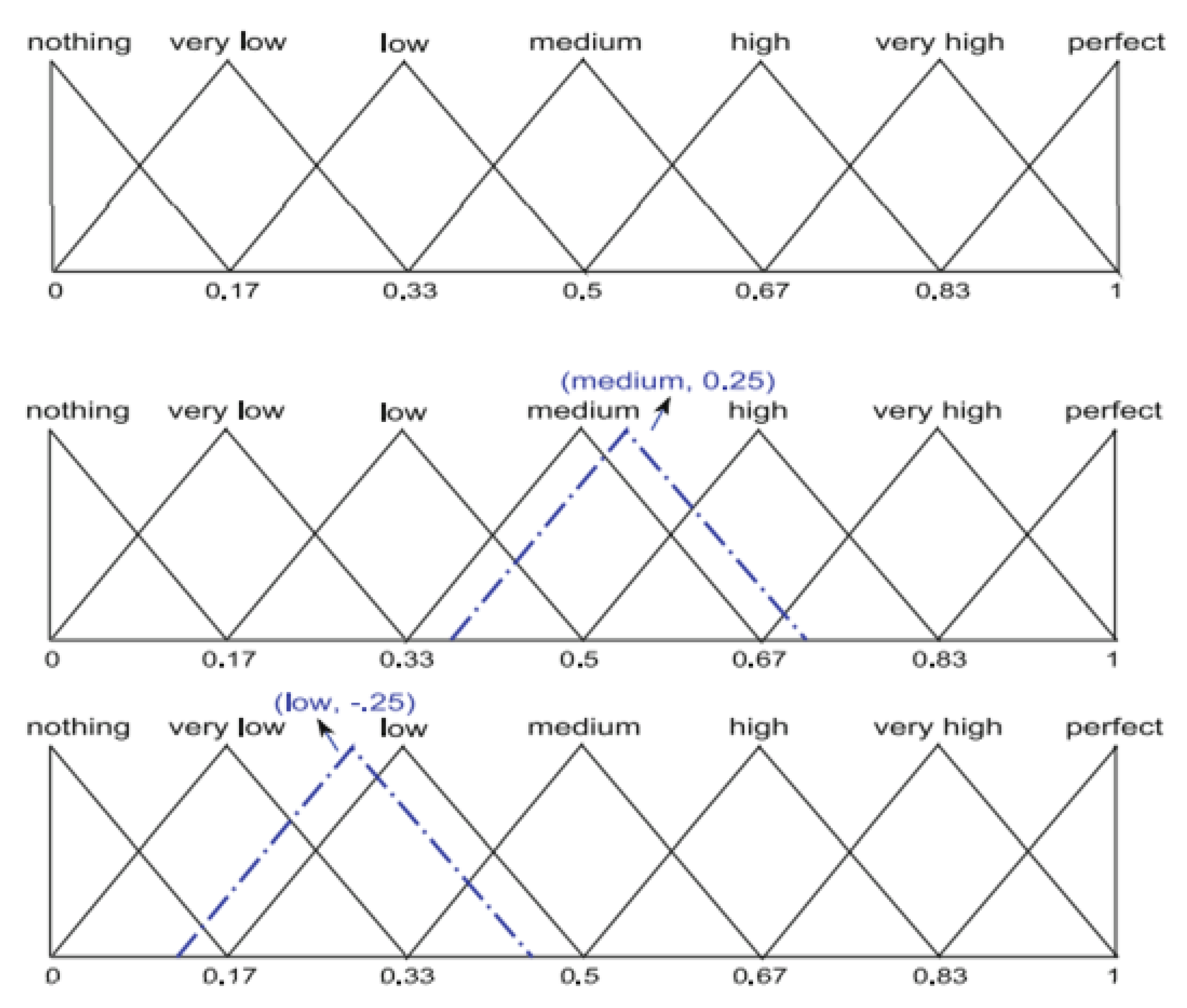
([22]). For a linguistic term set $S_{LT}=\left\{s_{S_{LT-0}},s_{S_{LT-1}},s_{S_{LT-2}},s_{S_{LT-3}},\dots .,s_{S_{LT-g}}\right\}$ with ${\beta }_{SC}\in \left[0,1\right]$, the 2-tuple linguistic function (2-TLF) Δ_LT is given by:

$${\Delta }_{LT}:\left[0,1\right]\to S_{LT}\times [-\frac{1}{2g},\frac{1}{2g}\}$$

(1)

$${\Delta }_{LT}\left({\beta }_{SC}\right)=\left(s_{S_{LT-j}},{\alpha }_{SC}\right) \mathrm{with} \{\begin{array}{cc}{s}_{S_{LT-j}}& j=round\left({\beta }_{SC},g\right)\\ {\alpha }_{SC}={\beta }_{SC}-\frac{j}{g}& {\alpha }_{SC}\in [-\frac{1}{2g},\frac{1}{2g}\}\end{array}$$

(2)

The 2-tuple linguistic inverse function${\Delta }_{LT}^{-1}$is given by:

$${\Delta }_{LT}^{-1}:S_{LT}\times [-\frac{1}{2g},\frac{1}{2g}\}\to \left[0,1\right]$$

(3)

$${\Delta }_{LT}^{-1}\left(s_{S_{LT-j}},{\alpha }_{SC}\right)=\frac{j}{g}+{\alpha }_{SC}={\beta }_{SC}$$

(4)

Example 1. 

Let a symbolic aggregation operator$\phi (.)$have different labels assessed in the linguistic term set S_LT = {nothing, very low; low; medium; high; very high, perfect}. If we have the following results:

$$\phi \left(high,high,high,very low\right)=0.75={\beta }_{SC-1} \mathrm{and} \phi \left(low,nothing,medium,low\right)=0.0833={\beta }_{SC-2},$$

then, by using the value of${\beta }_{SC-1}=0.75$and${\beta }_{SC-2}=0.0833$, we obtain the 2-tuple linguistic values of theses symbolic results that do not match with any linguistic term in$S_{LT}$with

$${\Delta }_{LT}\left(0.75\right)=\left(s_3,0.25\right)=\left(medium,0.25\right) \mathrm{and} {\Delta }_{LT}\left(0.0833\right)=\left(s_2,-0.25\right)=\left(low,-0.25\right).$$

The geometrical expressions are shown in Figure 1. From Figure 1, it is seen that the 2-tuple fuzzy linguistic representation model keeps the fuzzy representation and syntax according to the fuzzy linguistic approach.

It is known that 2-tuple linguistic aggregation operators had been considered by using fuzzy sets and their extensions. For coping with more sorts of fuzzy environments, the theory of QROF2-TLV with aggregation operators was proposed by Ju et al. [35]. We next review the definition of QROF2-TLV.

Definition 2 

([35]). A QROF2-TLV is given by

$${\mathcal{Q}}_{QTL}=\left\{\left(\left(s_{S_{LT}(ử)},{\alpha }_{SC}\right),\left({\mu }_{{\mathcal{Q}}_{QTL}}(ử),{\eta }_{{\mathcal{Q}}_{QTL}}(ử)\right)\right):ử\in {Ữ}_{UNI}\right\}$$

(5)

where ${\mu }_{{\mathcal{Q}}_Q}:{Ữ}_{UNI}\to \left[0,1\right]$ and ${\eta }_{{\mathcal{Q}}_Q}:{Ữ}_{UNI}\to \left[0,1\right]$, with a condition: $0\le {\mu }_{{\mathcal{Q}}_Q}^{q_{SC}}(ử)+{\eta }_{{\mathcal{Q}}_Q}^{q_{SC}}(ử)\le 1$ and the pair $\left(s_{S_{LT}(ử)},{\alpha }_{SC}\right)$, is called 2-tulpe linguistic variable with ${\alpha }_{SC}\in [-\frac{1}{2g},\frac{1}{2g}\}$ and $s_{S_{LT}(ử)}\in S_{LT}$. Moreover, ${\zeta }_{{\mathcal{Q}}_Q}(ử)=1-{\left({\mu }_{{\mathcal{Q}}_Q}^{q_{SC}}(ử)+{\eta }_{{\mathcal{Q}}_Q}^{q_{SC}}(ử)\right)}^{\frac{1}{q_{SC}}}$ is called refusal grade, and the q-rung orthopair fuzzy 2-tuple linguistic number (QROF2-TLN) is represented by ${\mathcal{Q}}_{QTL}=\left(\left(s_{S_{LT}(ử)},{\alpha }_{SC}\right),\left({\mu }_{{\mathcal{Q}}_{QTL}}(ử),{\eta }_{{\mathcal{Q}}_{QTL}}(ử)\right)\right)$.

Example 2. 

If a decision-maker provides 0.9 for truth grade, 0.7 for falsity grade, and $\left(s_3,0.25\right)$ for the 2-tuple linguistic term, then the QROF2-TLN is defined as ${\mathcal{Q}}_{QTL}=\left(\left(s_3,0.25\right),\left(0.9,0.7\right)\right)$ by using the value of q_CQ = 4.

Definition 3 

([35]). For any two QROF2-TLNs ${\mathcal{Q}}_{QTL-1}=\left(\left(s_{S_{LT-1}(ử)},{\alpha }_{SC-1}\right),\left({\mu }_{{\mathcal{Q}}_{QTL-1}}(ử),{\eta }_{{\mathcal{Q}}_{QTL-1}}(ử)\right)\right)$ and ${\mathcal{Q}}_{QTL-2}=\left(\left(s_{S_{LT-2}(ử)},{\alpha }_{SC-2}\right),\left({\mu }_{{\mathcal{Q}}_{QTL-2}}(ử),{\eta }_{{\mathcal{Q}}_{QTL-2}}(ử)\right)\right)$, then

• ${\mathcal{Q}}_{QTL-1}{\oplus }_{QTL}{\mathcal{Q}}_{QTL-2}=\left(\begin{array}{c}{\Delta }_{LT}\left({\Delta }_{LT}^{-1}\left(s_{S_{LT-1}(ử)},{\alpha }_{SC-1}\right)+{\Delta }_{LT}^{-1}\left(s_{S_{LT-2}(ử)},{\alpha }_{SC-2}\right)\right).\\ \left({\left(\begin{array}{c}{\mu }_{{\mathcal{Q}}_{QTL-1}}^{q_{CQ}}(ử)+{\mu }_{{\mathcal{Q}}_{QTL-2}}^{q_{CQ}}(ử)-\\ {\mu }_{{\mathcal{Q}}_{QTL-1}}^{q_{CQ}}(ử){\mu }_{{\mathcal{Q}}_{QTL-2}}^{q_{CQ}}(ử)\end{array}\right)}^{\frac{1}{q_{CQ}}},{\eta }_{{\mathcal{Q}}_{QTL-1}}(ử){\eta }_{{\mathcal{Q}}_{QTL-2}}(ử)\right)\end{array}\right)$;
• ${\mathcal{Q}}_{QTL-1}{\otimes }_{QTL}{\mathcal{Q}}_{QTL-2}=\left(\begin{array}{c}{\Delta }_{LT}\left({\Delta }_{LT}^{-1}\left(s_{S_{LT-1}(ử)},{\alpha }_{SC-1}\right)\times {\Delta }_{LT}^{-1}\left(s_{S_{LT-2}(ử)},{\alpha }_{SC-2}\right)\right).\\ \left({\mu }_{{\mathcal{Q}}_{QTL-1}}(ử){\mu }_{{\mathcal{Q}}_{QTL-2}}(ử),{\left(\begin{array}{c}{\eta }_{{\mathcal{Q}}_{QTL-1}}^{q_{CQ}}(ử)+{\eta }_{{\mathcal{Q}}_{QTL-2}}^{q_{CQ}}(ử)-\\ {\eta }_{{\mathcal{Q}}_{QTL-1}}^{q_{CQ}}(ử){\eta }_{{\mathcal{Q}}_{QTL-2}}^{q_{CQ}}(ử)\end{array}\right)}^{\frac{1}{q_{CQ}}}\right)\end{array}\right)$;
• ${\mathcal{Q}}_{QTL-1}^{{\delta }_{SC}}=\left({\Delta }_{LT}\left({\Delta }_{LT}^{-1}{\left(s_{S_{LT-1}(ử)},{\alpha }_{SC-1}\right)}^{{\delta }_{SC}}\right),\left({\mu }_{{\mathcal{Q}}_{QTL-1}}^{{\delta }_{SC}}(ử),{\left(1-{\left(1-{\eta }_{{\mathcal{Q}}_{QTL-1}}^{q_{CQ}}(ử)\right)}^{{\delta }_{SC}}\right)}^{\frac{1}{q_{CQ}}}\right)\right)$;
• ${\delta }_{SC}{\mathcal{Q}}_{QTL-1}=\left({\Delta }_{LT}\left({\delta }_{SC}\times {\Delta }_{LT}^{-1}\left(s_{S_{LT-1}(ử)},{\alpha }_{SC-1}\right)\right),\left({\left(1-{\left(1-{\mu }_{{\mathcal{Q}}_{QTL-1}}^{q_{CQ}}(ử)\right)}^{{\delta }_{SC}}\right)}^{\frac{1}{q_{CQ}}},{\eta }_{{\mathcal{Q}}_{QTL-1}}^{{\delta }_{SC}}(ử)\right)\right)$.

Example 3. 

Let${\mathcal{Q}}_{QTL-1}=\left(\left(s_2,0.01\right),\left(0.8,0.6\right)\right)$and${\mathcal{Q}}_{QTL-2}=\left(\left(s_4,-0.02\right),\left(0.9,0.4\right)\right)$be the two QROF2-TLNs, and the linguistic set be$S_{LT}=\left\{s_0,s_1,\dots .,s_4\right\}$for${\delta }_{SC}=2$and$q_{CQ}=2$. By Definition 3, we can obtain the following results:

• $\begin{array}{l}{\mathcal{Q}}_{QTL-1}{\oplus }_{QTL}{\mathcal{Q}}_{QTL-2}=\left(\begin{array}{c}{\Delta }_{LT}\left(\left(\frac{2}{4}+0.01\right)+\left(\frac{4}{4}-0.02\right)\right),\\ \left(\begin{array}{c}\left(0.9652\right),\\ \left(0.24\right)\end{array}\right)\end{array}\right)=\left(\begin{array}{c}{\Delta }_{LT}\left(1.49\right),\\ \left(\begin{array}{c}\left(0.9652\right),\\ \left(0.24\right)\end{array}\right)\end{array}\right)=\\ \left(\begin{array}{c}\left(s_{S_{LT-4}},0.49\right),\\ \left(\begin{array}{c}\left(0.9652\right),\\ \left(0.24\right)\end{array}\right)\end{array}\right).\end{array}$
• $\begin{array}{l}{\mathcal{Q}}_{QTL-1}{\otimes }_{QTL}{\mathcal{Q}}_{QTL-2}=\left(\begin{array}{c}{\Delta }_{LT}\left(\left(\frac{2}{4}+0.01\right)\times \left(\frac{4}{4}-0.02\right)\right),\\ \left(\begin{array}{c}\left(0.72\right),\\ \left(0.68\right)\end{array}\right)\end{array}\right)=\left(\begin{array}{c}{\Delta }_{LT}\left(0.4998\right),\\ \left(\begin{array}{c}\left(0.72\right),\\ \left(0.68\right)\end{array}\right)\end{array}\right)=\\ \left(\begin{array}{c}\left(s_{S_{LT-3}},0.1665\right),\\ \left(\begin{array}{c}\left(0.9652\right),\\ \left(0.24\right)\end{array}\right)\end{array}\right)\end{array}$.
• ${\mathcal{Q}}_{QTL-1}^2=\left(\begin{array}{c}{\Delta }_{LT}\left({\left(0.51\right)}^2\right),\\ \left(\begin{array}{c}0.64,\\ {\left(1-{\left(1-0.36\right)}^2\right)}^{\frac{1}{2}}\end{array}\right)\end{array}\right)=\left(\begin{array}{c}{\Delta }_{LT}\left(0.2601\right),\\ \left(\begin{array}{c}0.64,\\ 0.7684\end{array}\right)\end{array}\right)=\left(\begin{array}{c}\left(s_{S_{LT-1}},0.0101\right),\\ \left(\begin{array}{c}0.64,\\ 0.7684\end{array}\right)\end{array}\right)$.
• $2\times {\mathcal{Q}}_{QTL-1}=\left(\begin{array}{c}{\Delta }_{LT}\left(2\times 0.51\right),\\ \left(\begin{array}{c}{\left(1-{\left(1-0.64\right)}^2\right)}^{\frac{1}{2}},\\ {0.6}^2\end{array}\right)\end{array}\right)=\left(\begin{array}{c}{\Delta }_{LT}\left(1.02\right),\\ \left(\begin{array}{c}0.9330,\\ 0.36\end{array}\right)\end{array}\right)=\left(\begin{array}{c}\left(s_{S_{LT-4}},0.02\right),\\ \left(\begin{array}{c}0.9330,\\ 0.36\end{array}\right)\end{array}\right)$.

The score and accuracy functions are important for determining the relationships among attributes, we briefly review the score and accuracy functions of QROF2-TLNs as follows.

Definition 4 

([35]). For any two QROF2-TLNs ${\mathcal{Q}}_{QTL-1}=\left(\left(s_{S_{LT-1}(ử)},{\alpha }_{SC-1}\right),\left({\mu }_{{\mathcal{Q}}_{QTL-1}}(ử),{\eta }_{{\mathcal{Q}}_{QTL-1}}(ử)\right)\right)$ and ${\mathcal{Q}}_{QTL-2}=\left(\left(s_{S_{LT-2}(ử)},{\alpha }_{SC-2}\right),\left({\mu }_{{\mathcal{Q}}_{QTL-2}}(ử),{\eta }_{{\mathcal{Q}}_{QTL-2}}(ử)\right)\right)$, the score and accuracy functions are given by:

$$Ş\left({\mathcal{Q}}_{QTL-1}\right)=\frac{{\Delta }_{LT}^{-1}\left(s_{S_{LT-1}(ử)},{\alpha }_{SC-1}\right)\times \left(1+{\mu }_{{\mathcal{Q}}_{QTL-1}}^{q_{SC}}(ử)-{\eta }_{{\mathcal{Q}}_{QTL-1}}^{q_{SC}}(ử)\right)}{2}$$

(6)

$$Ȟ\left({\mathcal{Q}}_{QTL-1}\right)={\Delta }_{LT}^{-1}\left(s_{S_{LT-1}(ử)},{\alpha }_{SC-1}\right)\times \left({\mu }_{{\mathcal{Q}}_{QTL-1}}^{q_{SC}}(ử)+{\eta }_{{\mathcal{Q}}_{QTL-1}}^{q_{SC}}(ử)\right)$$

(7)

Based on the above two notions, the compassion between two QROF2-TLNs are given by:

• If $Ş\left({\mathcal{Q}}_{QTL-1}\right)>Ş\left({\mathcal{Q}}_{QTL-2}\right)$, then ${\mathcal{Q}}_{QTL-1}>{\mathcal{Q}}_{QTL-2}$;
• If $Ş\left({\mathcal{Q}}_{QTL-1}\right)=Ş\left({\mathcal{Q}}_{QTL-2}\right)$, then:

  (1)

  If $Ȟ\left({\mathcal{Q}}_{QTL-1}\right)>Ȟ\left({\mathcal{Q}}_{QTL-2}\right)$, then ${\mathcal{Q}}_{QTL-1}>{\mathcal{Q}}_{QTL-2}$;

  (2)

  If $Ȟ\left({\mathcal{Q}}_{QTL-1}\right)=Ȟ\left({\mathcal{Q}}_{QTL-2}\right)$, then ${\mathcal{Q}}_{QTL-1}={\mathcal{Q}}_{QTL-2}$.

In most of mean operators, the Maclurin symmetric mean (MSM) operators offer more flexible arrangement with its modifiable factors. Further, MSM aggregation operators perform a significant role in conveying the magnitude level of options and characteristics. Thus, we next review the definition of MSM operators.

Definition 5 

([36]). For a family of positive numbers ${\mathcal{Q}}_{CQ-j},j=1,2,3,\dots ,n$, the Maclurin symmetric mean (MSM) operator is given by

$$MS{M}^{K_{SC}}\left({\mathcal{Q}}_{CQ-1},{\mathcal{Q}}_{CQ-2},\dots ,{\mathcal{Q}}_{CQ-n}\right)={\left(\frac{{{\displaystyle \sum }}_{1\le j_1\le \dots \le j_{K_{SC}}}{{\displaystyle \prod }}_{i=1}^{K_{SC }}{\mathcal{Q}}_{CQ-j_i}}{C_n^{K_{SC}}}\right)}^{\frac{1}{K_{SC }}}$$

(8)

where $K_{SC}=1,2,\dots ,n,\left(j_1,j_2,\dots ,j_{K_{SC}}\right)$ denotes K-tuple family of $\left(1,2,\dots ,n\right),$ and the symbol $C_n^{K_{SC}}$denotes the binomial co-efficient, which holds the following conditions:

1. 

$MS{M}^{K_{SC}}\left({\mathcal{Q}}_{CQ},{\mathcal{Q}}_{CQ},\dots ,{\mathcal{Q}}_{CQ}\right)={\mathcal{Q}}_{CQ}$;

2. 

$MS{M}^{K_{SC}}\left({\mathcal{Q}}_{CQ-1},{\mathcal{Q}}_{CQ-2},\dots ,{\mathcal{Q}}_{CQ-n}\right)\le MS{M}^{K_{SC}}\left({\mathcal{Q}}_{CQ-*1},{\mathcal{Q}}_{CQ-*2},\dots ,{\mathcal{Q}}_{CQ-*n}\right)$, if${\mathcal{Q}}_{CQ-j}\le {\mathcal{Q}}_{CQ-*j}$for all j;

3. 

$\underset{j}{min}{\mathcal{Q}}_{CQ-j}\le MS{M}^{K_{SC}}\left({\mathcal{Q}}_{CQ-1},{\mathcal{Q}}_{CQ-2},\dots ,{\mathcal{Q}}_{CQ-n}\right)\le \underset{j}{max}{\mathcal{Q}}_{CQ-j}$.

We next give the review of a DTRS model for three-way decision (3WD). According to DTRS for 3WD, it contains two states and three actions with the state set ${\Omega }_S=\left\{{ℱ}_B,\sim {ℱ}_{NB}\right\}$ and the action set $A_{AC}=\left\{{\chi }_{P_{AC}},{\chi }_{B_{AC}},{\chi }_{N_{AC}}\right\}$. The symbols of the set ${\Omega }_S$ are used for belonging and for not belonging, and the symbols of the set $A_{AC}$ are used for positive, boundary, and negative. The symbol used for positive means to accept the event; the symbol used for negative means to reject the event; however, the symbol used for boundary means not to promise or just to delay the decision. Thus, these three decision cases correspond to three-way decisions. Further, based on Bayesian rules, these exist loss functions for risk when we take actions in different states. These loss functions are presented in

Table 1. Loss functions of DTRS for 3WD.

Symbols	${ℱ}_{\mathit{B}}\left({\mathit{P}}_{\mathit{A}\mathit{C}}\right)=\mathit{C}\mathit{o}\mathit{r}\mathit{r}\mathit{e}\mathit{c}\mathit{t}\mathit{l}\mathit{y} \mathit{S}\mathit{o}\mathit{l}\mathit{v}\mathit{e}\mathit{d}$	$\sim {ℱ}_{\mathit{N}\mathit{B}}\left({\mathit{N}}_{\mathit{A}\mathit{C}}\right)=\mathit{W}\mathit{r}\mathit{o}\mathit{n}\mathit{g}\mathit{l}\mathit{y} \mathit{S}\mathit{o}\mathit{l}\mathit{v}\mathit{e}\mathit{d}$
${\mathit{\chi }}_{{\mathit{P}}_{\mathit{A}\mathit{C}}}$	${\overline{\mathcal{Q}}}_{CQ-P_{AC}{P}_{AC}}$	${\overline{\mathcal{Q}}}_{CQ-P_{AC}{N}_{AC}}$
${\mathit{\chi }}_{{\mathit{B}}_{\mathit{A}\mathit{C}}}$	${\overline{\mathcal{Q}}}_{CQ-B_{AC}{P}_{AC}}$	${\overline{\mathcal{Q}}}_{CQ-B_{AC}{N}_{AC}}$
${\mathit{\chi }}_{{\mathit{N}}_{\mathit{A}\mathit{C}}}$	${\overline{\mathcal{Q}}}_{CQ-N_{AC}{P}_{AC}}$	${\overline{\mathcal{Q}}}_{CQ-N_{AC}{N}_{AC}}$
${\overline{\mathcal{Q}}}_{\mathit{C}\mathit{Q}-{\mathit{P}}_{\mathit{A}\mathit{C}}{\mathit{P}}_{\mathit{A}\mathit{C}}},{\overline{\mathcal{Q}}}_{\mathit{C}\mathit{Q}-{\mathit{P}}_{\mathit{A}\mathit{C}}{\mathit{N}}_{\mathit{A}\mathit{C}}}$ = Costs of the correct sort and error sort of the object $ử$ in accepted decision.
${\overline{\mathcal{Q}}}_{\mathit{C}\mathit{Q}-{\mathit{B}}_{\mathit{A}\mathit{C}}{\mathit{P}}_{\mathit{A}\mathit{C}}},{\overline{\mathcal{Q}}}_{\mathit{C}\mathit{Q}-{\mathit{B}}_{\mathit{A}\mathit{C}}{\mathit{N}}_{\mathit{A}\mathit{C}}}$ = Costs of the correct sort and error sort of the object $ử$ in delay decision.
${\overline{\mathcal{Q}}}_{\mathit{C}\mathit{Q}-{\mathit{N}}_{\mathit{A}\mathit{C}}{\mathit{P}}_{\mathit{A}\mathit{C}}},{\overline{\mathcal{Q}}}_{\mathit{C}\mathit{Q}-{\mathit{N}}_{\mathit{A}\mathit{C}}{\mathit{N}}_{\mathit{A}\mathit{C}}}$ = Costs of the correct sort and error sort of the object $ử$ in rejected decision.

.

From Table 1, there are the following inequalities:

$${\overline{\mathcal{Q}}}_{CQ-P_{AC}{P}_{AC}}<{\overline{\mathcal{Q}}}_{CQ-B_{AC}{P}_{AC}}<{\overline{\mathcal{Q}}}_{CQ-N_{AC}{P}_{AC}}$$

(9)

$${\overline{\mathcal{Q}}}_{CQ-N_{AC}{N}_{AC}}<{\overline{\mathcal{Q}}}_{CQ-B_{AC}{N}_{AC}}<{\overline{\mathcal{Q}}}_{CQ-P_{AC}{N}_{AC}}$$

(10)

Based on Bayesian decision theory, we have

$$\mathrm{Pr}\left({ℱ}_B|[ử]\right)+\mathrm{Pr}\left(\sim {ℱ}_{NB}|[ử]\right)=1$$

(11)

According to Equation (11), the expected loss $Y_{EL}\left({\chi }_{j_{AC}}|[ử]\right),j=P,B,N$, for different actions can be expressed as follows:

$$Y_{EL}\left({\chi }_{P_{AC}}|[ử]\right)={\overline{\mathcal{Q}}}_{CQ-P_{AC}{P}_{AC}}\mathrm{Pr}\left({ℱ}_B|[ử]\right)+{\overline{\mathcal{Q}}}_{CQ-P_{AC}{N}_{AC}}\mathrm{Pr}\left(\sim {ℱ}_{NB}|[ử]\right)$$

(12)

$$Y_{EL}\left({\chi }_{B_{AC}}|[ử]\right)={\overline{\mathcal{Q}}}_{CQ-B_{AC}{P}_{AC}}\mathrm{Pr}\left({ℱ}_B|[ử]\right)+{\overline{\mathcal{Q}}}_{CQ-B_{AC}{N}_{AC}}\mathrm{Pr}\left(\sim {ℱ}_{NB}|[ử]\right)$$

(13)

$$Y_{EL}\left({\chi }_{N_{AC}}|[ử]\right)={\overline{\mathcal{Q}}}_{CQ-N_{AC}{P}_{AC}}\mathrm{Pr}\left({ℱ}_B|[ử]\right)+{\overline{\mathcal{Q}}}_{CQ-N_{AC}{N}_{AC}}\mathrm{Pr}\left(\sim {ℱ}_{NB}|[ử]\right)$$

(14)

Thus, the three-way decision rules are presented as follows:

$$\begin{gathered} P_{AC}: \mathrm{If} Y_{EL}\left({\chi }_{P_{AC}}|[ử]\right)\le Y_{EL}\left({\chi }_{B_{AC}}|[ử]\right) \mathrm{and} Y_{EL}\left({\chi }_{P_{AC}}|[ử]\right)\le Y_{EL}\left({\chi }_{N_{AC}}|[ử]\right), \\ \mathrm{then} ử\in POS\left({ℱ}_P\right); \end{gathered}$$

(15)

$$\begin{gathered} B_{AC}: \mathrm{If} Y_{EL}\left({\chi }_{B_{AC}}|[ử]\right)\le Y_{EL}\left({\chi }_{P_{AC}}|[ử]\right) \mathrm{and} Y_{EL}\left({\chi }_{B_{AC}}|[ử]\right)\le Y_{EL}\left({\chi }_{N_{AC}}|[ử]\right), \\ \mathrm{then} ử\in BUN\left({ℱ}_B\right); \end{gathered}$$

(16)

$$\begin{gathered} N_{AC}: \mathrm{If} Y_{EL}\left({\chi }_{N_{AC}}|[ử]\right)\le Y_{EL}\left({\chi }_{P_{AC}}|[ử]\right) \mathrm{and} Y_{EL}\left({\chi }_{N_{AC}}|[ử]\right)\le Y_{EL}\left({\chi }_{B_{AC}}|[ử]\right), \\ \mathrm{then} ử\in NRG\left({ℱ}_N\right). \end{gathered}$$

(17)

3. The Proposed DTRS Model Based on Q-Rung Orthopair Fuzzy 2-Tuple Linguistic Variables

In this section, we propose a novel DTRS model for three-way decision (3WD) by using loss functions based on the q-rung orthopair fuzzy 2-tuple linguistic variable (QROF2-TLV). We call it QROF2-TLV-DTRS. We first construct these loss functions for risk when we take actions in different states under the proposed QROF2-TLV-DTRS. The loss functions of QROF2-TLV-DTRS are presented in

Table 2. Loss functions of QROF2-TLV-DTRS.

Symbols	${ℱ}_{\mathit{B}}\left({\mathit{P}}_{\mathit{A}\mathit{C}}\right)=\mathit{C}\mathit{o}\mathit{r}\mathit{r}\mathit{e}\mathit{c}\mathit{t}\mathit{l}\mathit{y} \mathit{s}\mathit{o}\mathit{l}\mathit{v}\mathit{e}\mathit{d}$	$\sim {ℱ}_{\mathit{N}\mathit{B}}\left({\mathit{N}}_{\mathit{A}\mathit{C}}\right)=\mathit{w}\mathit{r}\mathit{o}\mathit{n}\mathit{g}\mathit{l}\mathit{y} \mathit{s}\mathit{o}\mathit{l}\mathit{v}\mathit{e}\mathit{d}$
${\mathit{\chi }}_{{\mathit{P}}_{\mathit{A}\mathit{C}}}$	${\mathcal{Q}}_{QTL-{\overline{\mathcal{Q}}}_{CQ-P_{AC}{P}_{AC}}}=\left(\begin{array}{c}\left(s_{S_{LT}\left({\overline{\mathcal{Q}}}_{CQ-P_{AC}{P}_{AC}}\right)},{\alpha }_{SC}\right),\\ \left(\begin{array}{c}{\mu }_{{\mathcal{Q}}_{QTL}}\left({\overline{\mathcal{Q}}}_{CQ-P_{AC}{P}_{AC}}\right),\\ {\eta }_{{\mathcal{Q}}_{QTL}}\left({\overline{\mathcal{Q}}}_{CQ-P_{AC}{P}_{AC}}\right)\end{array}\right)\end{array}\right)$	${\mathcal{Q}}_{QTL-{\overline{\mathcal{Q}}}_{CQ-P_{AC}{N}_{AC}}}=\left(\begin{array}{c}\left(s_{S_{LT}\left({\overline{\mathcal{Q}}}_{CQ-P_{AC}{N}_{AC}}\right)},{\alpha }_{SC}\right),\\ \left(\begin{array}{c}{\mu }_{{\mathcal{Q}}_{QTL}}\left({\overline{\mathcal{Q}}}_{CQ-N_{AC}{P}_{AC}}\right),\\ {\eta }_{{\mathcal{Q}}_{QTL}}\left({\overline{\mathcal{Q}}}_{CQ-N_{AC}{P}_{AC}}\right)\end{array}\right)\end{array}\right)$
${\mathit{\chi }}_{{\mathit{B}}_{\mathit{A}\mathit{C}}}$	${\mathcal{Q}}_{QTL-{\overline{\mathcal{Q}}}_{CQ-B_{AC}{P}_{AC}}}=\left(\begin{array}{c}\left(s_{S_{LT}\left({\overline{\mathcal{Q}}}_{CQ-B_{AC}{P}_{AC}}\right)},{\alpha }_{SC}\right),\\ \left(\begin{array}{c}{\mu }_{{\mathcal{Q}}_{QTL}}\left({\overline{\mathcal{Q}}}_{CQ-B_{AC}{P}_{AC}}\right),\\ {\eta }_{{\mathcal{Q}}_{QTL}}\left({\overline{\mathcal{Q}}}_{CQ-B_{AC}{P}_{AC}}\right)\end{array}\right)\end{array}\right)$	${\mathcal{Q}}_{QTL-{\overline{\mathcal{Q}}}_{CQ-B_{AC}{N}_{AC}}}=\left(\begin{array}{c}\left(s_{S_{LT}\left({\overline{\mathcal{Q}}}_{CQ-B_{AC}{N}_{AC}}\right)},{\alpha }_{SC}\right),\\ \left(\begin{array}{c}{\mu }_{{\mathcal{Q}}_{QTL}}\left({\overline{\mathcal{Q}}}_{CQ-B_{AC}{N}_{AC}}\right),\\ {\eta }_{{\mathcal{Q}}_{QTL}}\left({\overline{\mathcal{Q}}}_{CQ-B_{AC}{N}_{AC}}\right)\end{array}\right)\end{array}\right)$
${\mathit{\chi }}_{{\mathit{N}}_{\mathit{A}\mathit{C}}}$	${\mathcal{Q}}_{QTL-{\overline{\mathcal{Q}}}_{CQ-N_{AC}{P}_{AC}}}=\left(\begin{array}{c}\left(s_{S_{LT}\left({\overline{\mathcal{Q}}}_{CQ-N_{AC}{P}_{AC}}\right)},{\alpha }_{SC}\right),\\ \left(\begin{array}{c}{\mu }_{{\mathcal{Q}}_{QTL}}\left({\overline{\mathcal{Q}}}_{CQ-N_{AC}{P}_{AC}}\right),\\ {\eta }_{{\mathcal{Q}}_{QTL}}\left({\overline{\mathcal{Q}}}_{CQ-N_{AC}{P}_{AC}}\right)\end{array}\right)\end{array}\right)$	${\mathcal{Q}}_{QTL-{\overline{\mathcal{Q}}}_{CQ-N_{AC}{N}_{AC}}}=\left(\begin{array}{c}\left(s_{S_{LT}\left({\overline{\mathcal{Q}}}_{CQ-N_{AC}{N}_{AC}}\right)},{\alpha }_{SC}\right),\\ \left(\begin{array}{c}{\mu }_{{\mathcal{Q}}_{QTL}}\left({\overline{\mathcal{Q}}}_{CQ-N_{AC}{N}_{AC}}\right),\\ {\eta }_{{\mathcal{Q}}_{QTL}}\left({\overline{\mathcal{Q}}}_{CQ-N_{AC}{N}_{AC}}\right)\end{array}\right)\end{array}\right)$
${\mathcal{Q}}_{\mathit{Q}\mathit{T}\mathit{L}-{\overline{\mathcal{Q}}}_{\mathit{C}\mathit{Q}-{\mathit{P}}_{\mathit{A}\mathit{C}}{\mathit{P}}_{\mathit{A}\mathit{C}}}},{\mathcal{Q}}_{\mathit{Q}\mathit{T}\mathit{L}-{\overline{\mathcal{Q}}}_{\mathit{C}\mathit{Q}-{\mathit{P}}_{\mathit{A}\mathit{C}}{\mathit{N}}_{\mathit{A}\mathit{C}}}}$ = Costs of the correct sort and error sort of the object $ử$ in accepted decision.
${\mathcal{Q}}_{\mathit{Q}\mathit{T}\mathit{L}-{\overline{\mathcal{Q}}}_{\mathit{C}\mathit{Q}-{\mathit{B}}_{\mathit{A}\mathit{C}}{\mathit{P}}_{\mathit{A}\mathit{C}}}},{\mathcal{Q}}_{\mathit{Q}\mathit{T}\mathit{L}-{\overline{\mathcal{Q}}}_{\mathit{C}\mathit{Q}-{\mathit{B}}_{\mathit{A}\mathit{C}}{\mathit{N}}_{\mathit{A}\mathit{C}}}}$ = Costs of the correct sort and error sort of the object $ử$ in delay decision.
${\mathcal{Q}}_{\mathit{Q}\mathit{T}\mathit{L}-{\overline{\mathcal{Q}}}_{\mathit{C}\mathit{Q}-{\mathit{N}}_{\mathit{A}\mathit{C}}{\mathit{P}}_{\mathit{A}\mathit{C}}}},{\mathcal{Q}}_{\mathit{Q}\mathit{T}\mathit{L}-{\overline{\mathcal{Q}}}_{\mathit{C}\mathit{Q}-{\mathit{N}}_{\mathit{A}\mathit{C}}{\mathit{N}}_{\mathit{A}\mathit{C}}}}$ = Costs of the correct sort and error sort of the object $ử$ in rejected decision.
${\mathcal{Q}}_{QTL-{\overline{\mathcal{Q}}}_{CQ-P_{AC}{P}_{AC}}},{\mathcal{Q}}_{QTL-{\overline{\mathcal{Q}}}_{CQ-P_{AC}{N}_{AC}}}$ = Costs of the correct sort and error sort of the object $ử$ in accepted decision.
${\mathcal{Q}}_{QTL-{\overline{\mathcal{Q}}}_{CQ-B_{AC}{P}_{AC}}},{\mathcal{Q}}_{QTL-{\overline{\mathcal{Q}}}_{CQ-B_{AC}{N}_{AC}}}$ = Costs of the correct sort and error sort of the object $ử$ in delay decision.
${\mathcal{Q}}_{QTL-{\overline{\mathcal{Q}}}_{CQ-N_{AC}{P}_{AC}}},{\mathcal{Q}}_{QTL-{\overline{\mathcal{Q}}}_{CQ-N_{AC}{N}_{AC}}}$ = Costs of the correct sort and error sort of the object $ử$ in rejected decision.

.

From Table 2, we can obtain the following inequalities:

$${\mathcal{Q}}_{QTL-{\overline{\mathcal{Q}}}_{CQ-P_{AC}{P}_{AC}}}<{\mathcal{Q}}_{QTL-{\overline{\mathcal{Q}}}_{CQ-B_{AC}{P}_{AC}}}<{\mathcal{Q}}_{QTL-{\overline{\mathcal{Q}}}_{CQ-N_{AC}{P}_{AC}}}$$

(18)

$${\mathcal{Q}}_{QTL-{\overline{\mathcal{Q}}}_{CQ-N_{AC}{N}_{AC}}}<{\mathcal{Q}}_{QTL-{\overline{\mathcal{Q}}}_{CQ-B_{AC}{N}_{AC}}}<{\mathcal{Q}}_{QTL-{\overline{\mathcal{Q}}}_{CQ-P_{AC}{N}_{AC}}}$$

(19)

Further, the expected losses $Y_{EL}\left({\chi }_{j_{AC}}|[ử]\right),j=P,B,N,$ in QROF2-TLV-DTRS with different actions are expressed as follows:

$$Y_{EL}\left({\chi }_{P_{AC}}|[ử]\right)={\mathcal{Q}}_{QTL-{\overline{\mathcal{Q}}}_{CQ-P_{AC}{P}_{AC}}}\mathrm{Pr}\left({ℱ}_B|[ử]\right){\oplus }_{QTL}{\mathcal{Q}}_{QTL-{\overline{\mathcal{Q}}}_{CQ-P_{AC}{P}_{AC}}}\mathrm{Pr}\left(\sim {ℱ}_{NB}|[ử]\right)$$

(20)

$$Y_{EL}\left({\chi }_{B_{AC}}|[ử]\right)={\mathcal{Q}}_{QTL-{\overline{\mathcal{Q}}}_{CQ-B_{AC}{P}_{AC}}}\mathrm{Pr}\left({ℱ}_B|[ử]\right){\oplus }_{QTL}{\mathcal{Q}}_{QTL-{\overline{\mathcal{Q}}}_{CQ-B_{AC}{N}_{AC}}}\mathrm{Pr}\left(\sim {ℱ}_{NB}|[ử]\right)$$

(21)

$$Y_{EL}\left({\chi }_{N_{AC}}|[ử]\right)={\mathcal{Q}}_{QTL-{\overline{\mathcal{Q}}}_{CQ-N_{AC}{P}_{AC}}}\mathrm{Pr}\left({ℱ}_B|[ử]\right){\oplus }_{QTL}{\mathcal{Q}}_{QTL-{\overline{\mathcal{Q}}}_{CQ-N_{AC}{N}_{AC}}}\mathrm{Pr}\left(\sim {ℱ}_{NB}|[ử]\right)$$

(22)

For simple symbols, we use $\mathrm{Pr}\left({ℱ}_B|[ử]\right)={\delta }_B$ and $\mathrm{Pr}\left(\sim {ℱ}_{NB}|[ử]\right)={\delta }_{NB}$, and so ${\delta }_B+{\delta }_{NB}=1$. Thus, we obtain the following results.

Theorem 1. 

By using the expected losses of Equations (20)–(22), we get

$$Y_{EL}\left({\chi }_{P_{AC}}|[ử]\right)=\left(\begin{array}{c}{\Delta }_{LT}\left({\delta }_B\times {\Delta }_{LT}^{-1}\left(s_{S_{LT}\left({\overline{\mathcal{Q}}}_{CQ-P_{AC}{P}_{AC}}\right)},{\alpha }_{SC}\right)+{\delta }_{NB}\times {\Delta }_{LT}^{-1}\left(s_{S_{LT}\left({\overline{\mathcal{Q}}}_{CQ-P_{AC}{N}_{AC}}\right)},{\alpha }_{SC}\right)\right),\\ \left(\begin{array}{c}{\left(1-{\left(1-{\mu }_{{\mathcal{Q}}_{QTL}}^{q_{CQ}}\left({\overline{\mathcal{Q}}}_{CQ-P_{AC}{P}_{AC}}\right)\right)}^{{\delta }_B}{\left(1-{\mu }_{{\mathcal{Q}}_{QTL}}^{q_{CQ}}\left({\overline{\mathcal{Q}}}_{CQ-P_{AC}{N}_{AC}}\right)\right)}^{{\delta }_{NB}}\right)}^{\frac{1}{q_{CQ}}},\\ {\left({\eta }_{{\mathcal{Q}}_{QTL}}\left({\overline{\mathcal{Q}}}_{CQ-P_{AC}{P}_{AC}}\right)\right)}^{{\delta }_B}{\left({\eta }_{{\mathcal{Q}}_{QTL}}\left({\overline{\mathcal{Q}}}_{CQ-P_{AC}{N}_{AC}}\right)\right)}^{{\delta }_{NB}}\end{array}\right)\end{array}\right)$$

(23)

$$Y_{EL}\left({\chi }_{B_{AC}}|[ử]\right)=\left(\begin{array}{c}{\Delta }_{LT}\left({\delta }_B\times {\Delta }_{LT}^{-1}\left(s_{S_{LT}\left({\overline{\mathcal{Q}}}_{CQ-B_{AC}{P}_{AC}}\right)},{\alpha }_{SC}\right)+{\delta }_{NB}\times {\Delta }_{LT}^{-1}\left(s_{S_{LT}\left({\overline{\mathcal{Q}}}_{CQ-B_{AC}{N}_{AC}}\right)},{\alpha }_{SC}\right)\right),\\ \left(\begin{array}{c}{\left(1-{\left(1-{\mu }_{{\mathcal{Q}}_{QTL}}^{q_{CQ}}\left({\overline{\mathcal{Q}}}_{CQ-B_{AC}{P}_{AC}}\right)\right)}^{{\delta }_B}{\left(1-{\mu }_{{\mathcal{Q}}_{QTL}}^{q_{CQ}}\left({\overline{\mathcal{Q}}}_{CQ-B_{AC}{N}_{AC}}\right)\right)}^{{\delta }_{NB}}\right)}^{\frac{1}{q_{CQ}}},\\ {\left({\eta }_{{\mathcal{Q}}_{QTL}}\left({\overline{\mathcal{Q}}}_{CQ-B_{AC}{P}_{AC}}\right)\right)}^{{\delta }_B}{\left({\eta }_{{\mathcal{Q}}_{QTL}}\left({\overline{\mathcal{Q}}}_{CQ-B_{AC}{N}_{AC}}\right)\right)}^{{\delta }_{NB}}\end{array}\right)\end{array}\right)$$

(24)

$$Y_{EL}\left({\chi }_{N_{AC}}|[ử]\right)=\left(\begin{array}{c}{\Delta }_{LT}\left({\delta }_B\times {\Delta }_{LT}^{-1}\left(s_{S_{LT}\left({\overline{\mathcal{Q}}}_{CQ-N_{AC}{P}_{AC}}\right)},{\alpha }_{SC}\right)+{\delta }_{NB}\times {\Delta }_{LT}^{-1}\left(s_{S_{LT}\left({\overline{\mathcal{Q}}}_{CQ-N_{AC}{N}_{AC}}\right)},{\alpha }_{SC}\right)\right),\\ \left(\begin{array}{c}{\left(1-{\left(1-{\mu }_{{\mathcal{Q}}_{QTL}}^{q_{CQ}}\left({\overline{\mathcal{Q}}}_{CQ-N_{AC}{P}_{AC}}\right)\right)}^{{\delta }_B}{\left(1-{\mu }_{{\mathcal{Q}}_{QTL}}^{q_{CQ}}\left({\overline{\mathcal{Q}}}_{CQ-N_{AC}{N}_{AC}}\right)\right)}^{{\delta }_{NB}}\right)}^{\frac{1}{q_{CQ}}},\\ {\left({\eta }_{{\mathcal{Q}}_{QTL}}\left({\overline{\mathcal{Q}}}_{CQ-N_{AC}{P}_{AC}}\right)\right)}^{{\delta }_B}{\left({\eta }_{{\mathcal{Q}}_{QTL}}\left({\overline{\mathcal{Q}}}_{CQ-N_{AC}{N}_{AC}}\right)\right)}^{{\delta }_{NB}}\end{array}\right)\end{array}\right)$$

(25)

Proof. 

We only prove Equation (23). The proofs of Equations (24) and (25) are similar as that of Equation (23).

$$\begin{array}{ll}{Y}_{EL}\left({\chi }_{P_{AC}}|[ử]\right)& ={\mathcal{Q}}_{QTL-{\overline{\mathcal{Q}}}_{CQ-P_{AC}{P}_{AC}}}\mathrm{Pr}\left({ℱ}_B|[ử]\right){\oplus }_{QTL}{\mathcal{Q}}_{QTL-{\overline{\mathcal{Q}}}_{CQ-P_{AC}{P}_{AC}}}\mathrm{Pr}\left(\sim {ℱ}_{NB}|[ử]\right)\\ & ={\mathcal{Q}}_{QTL-{\overline{\mathcal{Q}}}_{CQ-P_{AC}{P}_{AC}}}{\delta }_B{\oplus }_{QTL}{\mathcal{Q}}_{QTL-{\overline{\mathcal{Q}}}_{CQ-P_{AC}{P}_{AC}}}{\delta }_{NB}\\ & =\left(\begin{array}{c}\left(\begin{array}{c}{\Delta }_{LT}\left({\delta }_B\times {\Delta }_{LT}^{-1}\left(s_{S_{LT}\left({\overline{\mathcal{Q}}}_{CQ-P_{AC}{P}_{AC}}\right)},{\alpha }_{SC}\right)\right),\\ \left(\begin{array}{c}{\left(1-{\left(1-{\mu }_{{\mathcal{Q}}_{QTL}}^{q_{CQ}}\left({\overline{\mathcal{Q}}}_{CQ-P_{AC}{P}_{AC}}\right)\right)}^{{\delta }_B}\right)}^{\frac{1}{q_{CQ}}},\\ {\left({\eta }_{{\mathcal{Q}}_{QTL}}\left({\overline{\mathcal{Q}}}_{CQ-P_{AC}{P}_{AC}}\right)\right)}^{{\delta }_B}\end{array}\right)\end{array}\right){\oplus }_{QTL}\\ \left(\begin{array}{c}{\Delta }_{LT}\left({\delta }_{NB}\times {\Delta }_{LT}^{-1}\left(s_{S_{LT}\left({\overline{\mathcal{Q}}}_{CQ-P_{AC}{N}_{AC}}\right)},{\alpha }_{SC}\right)\right),\\ \left(\begin{array}{c}{\left(1-{\left(1-{\mu }_{{\mathcal{Q}}_{QTL}}^{q_{CQ}}\left({\overline{\mathcal{Q}}}_{CQ-P_{AC}{N}_{AC}}\right)\right)}^{{\delta }_{NB}}\right)}^{\frac{1}{q_{CQ}}},\\ {\left({\eta }_{{\mathcal{Q}}_{QTL}}\left({\overline{\mathcal{Q}}}_{CQ-P_{AC}{N}_{AC}}\right)\right)}^{{\delta }_{NB}}\end{array}\right)\end{array}\right)\end{array}\right)\\ & =\left(\begin{array}{c}{\Delta }_{LT}\left({\delta }_B\times {\Delta }_{LT}^{-1}\left(s_{S_{LT}\left({\overline{\mathcal{Q}}}_{CQ-P_{AC}{P}_{AC}}\right)},{\alpha }_{SC}\right)+{\delta }_{NB}\times {\Delta }_{LT}^{-1}\left(s_{S_{LT}\left({\overline{\mathcal{Q}}}_{CQ-P_{AC}{N}_{AC}}\right)},{\alpha }_{SC}\right)\right),\\ \left(\begin{array}{c}{\left(1-{\left(1-{\mu }_{{\mathcal{Q}}_{QTL}}^{q_{CQ}}\left({\overline{\mathcal{Q}}}_{CQ-P_{AC}{P}_{AC}}\right)\right)}^{{\delta }_B}{\left(1-{\mu }_{{\mathcal{Q}}_{QTL}}^{q_{CQ}}\left({\overline{\mathcal{Q}}}_{CQ-P_{AC}{N}_{AC}}\right)\right)}^{{\delta }_{NB}}\right)}^{\frac{1}{q_{CQ}}},\\ {\left({\eta }_{{\mathcal{Q}}_{QTL}}\left({\overline{\mathcal{Q}}}_{CQ-P_{AC}{P}_{AC}}\right)\right)}^{{\delta }_B}{\left({\eta }_{{\mathcal{Q}}_{QTL}}\left({\overline{\mathcal{Q}}}_{CQ-P_{AC}{N}_{AC}}\right)\right)}^{{\delta }_{NB}}\end{array}\right)\end{array}\right)\end{array}$$

Thus, the proof is completed. □

Furthermore, the relationships between any two expected losses of $Y_{EL}\left({\chi }_{j_{AC}}|[ử]\right),j=P,B,N,$ in QROF2-TLV-DTRS can be obtained as follows:

$$Q_{EV}\left(Y_{EL}\left({\chi }_{P_{AC}}|[ử]\right)\right)=\frac{\left(\left(\begin{array}{c}{\delta }_B\times {\Delta }_{LT}^{-1}\left(s_{S_{LT}\left({\overline{\mathcal{Q}}}_{CQ-P_{AC}{P}_{AC}}\right)},{\alpha }_{SC}\right)+\\ {\delta }_{NB}\times {\Delta }_{LT}^{-1}\left(s_{S_{LT}\left({\overline{\mathcal{Q}}}_{CQ-P_{AC}{N}_{AC}}\right)},{\alpha }_{SC}\right)\end{array}\right)\times \left(\begin{array}{c}{\left(1-{\left(1-{\mu }_{{\mathcal{Q}}_{QTL}}^{q_{CQ}}\left({\overline{\mathcal{Q}}}_{CQ-P_{AC}{P}_{AC}}\right)\right)}^{{\delta }_B}{\left(1-{\mu }_{{\mathcal{Q}}_{QTL}}^{q_{CQ}}\left({\overline{\mathcal{Q}}}_{CQ-P_{AC}{N}_{AC}}\right)\right)}^{{\delta }_{NB}}\right)}^{\frac{1}{q_{CQ}}}+\\ {\left({\eta }_{{\mathcal{Q}}_{QTL}}\left({\overline{\mathcal{Q}}}_{CQ-P_{AC}{P}_{AC}}\right)\right)}^{{\delta }_B}{\left({\eta }_{{\mathcal{Q}}_{QTL}}\left({\overline{\mathcal{Q}}}_{CQ-P_{AC}{N}_{AC}}\right)\right)}^{{\delta }_{NB}}\end{array}\right)\right)}{4}$$

(26)

$$Q_{EV}\left(Y_{EL}\left({\chi }_{B_{AC}}|[ử]\right)\right)=\frac{\left(\left(\begin{array}{c}{\delta }_B\times {\Delta }_{LT}^{-1}\left(s_{S_{LT}\left({\overline{\mathcal{Q}}}_{CQ-B_{AC}{P}_{AC}}\right)},{\alpha }_{SC}\right)+\\ {\delta }_{NB}\times {\Delta }_{LT}^{-1}\left(s_{S_{LT}\left({\overline{\mathcal{Q}}}_{CQ-B_{AC}{N}_{AC}}\right)},{\alpha }_{SC}\right)\end{array}\right)\times \left(\begin{array}{c}{\left(1-{\left(1-{\mu }_{{\mathcal{Q}}_{QTL}}^{q_{CQ}}\left({\overline{\mathcal{Q}}}_{CQ-B_{AC}{P}_{AC}}\right)\right)}^{{\delta }_B}{\left(1-{\mu }_{{\mathcal{Q}}_{QTL}}^{q_{CQ}}\left({\overline{\mathcal{Q}}}_{CQ-B_{AC}{N}_{AC}}\right)\right)}^{{\delta }_{NB}}\right)}^{\frac{1}{q_{CQ}}}-\\ {\left({\eta }_{{\mathcal{Q}}_{QTL}}\left({\overline{\mathcal{Q}}}_{CQ-B_{AC}{P}_{AC}}\right)\right)}^{{\delta }_B}{\left({\eta }_{{\mathcal{Q}}_{QTL}}\left({\overline{\mathcal{Q}}}_{CQ-B_{AC}{N}_{AC}}\right)\right)}^{{\delta }_{NB}}\end{array}\right)\right)}{4}$$

(27)

$$Q_{EV}\left(Y_{EL}\left({\chi }_{D_{AC}}|[ử]\right)\right)=\frac{\left(\left(\begin{array}{c}{\delta }_B\times {\Delta }_{LT}^{-1}\left(s_{S_{LT}\left({\overline{\mathcal{Q}}}_{CQ-N_{AC}{P}_{AC}}\right)},{\alpha }_{SC}\right)+\\ {\delta }_{NB}\times {\Delta }_{LT}^{-1}\left(s_{S_{LT}\left({\overline{\mathcal{Q}}}_{CQ-N_{AC}{N}_{AC}}\right)},{\alpha }_{SC}\right)\end{array}\right)\times \left(\begin{array}{c}{\left(1-{\left(1-{\mu }_{{\mathcal{Q}}_{QTL}}^{q_{CQ}}\left({\overline{\mathcal{Q}}}_{CQ-N_{AC}{P}_{AC}}\right)\right)}^{{\delta }_B}{\left(1-{\mu }_{{\mathcal{Q}}_{QTL}}^{q_{CQ}}\left({\overline{\mathcal{Q}}}_{CQ-N_{AC}{N}_{AC}}\right)\right)}^{{\delta }_{NB}}\right)}^{\frac{1}{q_{CQ}}}-\\ {\left({\eta }_{{\mathcal{Q}}_{QTL}}\left({\overline{\mathcal{Q}}}_{CQ-N_{AC}{P}_{AC}}\right)\right)}^{{\delta }_B}{\left({\eta }_{{\mathcal{Q}}_{QTL}}\left({\overline{\mathcal{Q}}}_{CQ-N_{AC}{N}_{AC}}\right)\right)}^{{\delta }_{NB}}\end{array}\right)\right)}{4}$$

(28)

When the expected values fail to find the relationships between any two expected losses. For these kind of issues, we explore the notions of accuracy functions in QROF2-TLV-DTRS as follows:

$$G_{AF}\left(Y_{EL}\left({\chi }_{P_{AC}}|[ử]\right)\right)=\frac{\left(\left(\begin{array}{c}{\delta }_B\times {\Delta }_{LT}^{-1}\left(s_{S_{LT}\left({\overline{\mathcal{Q}}}_{CQ-P_{AC}{P}_{AC}}\right)},{\alpha }_{SC}\right)+\\ {\delta }_{NB}\times {\Delta }_{LT}^{-1}\left(s_{S_{LT}\left({\overline{\mathcal{Q}}}_{CQ-P_{AC}{N}_{AC}}\right)},{\alpha }_{SC}\right)\end{array}\right)\times \left(\begin{array}{c}{\left(1-{\left(1-{\mu }_{{\mathcal{Q}}_{QTL}}^{q_{CQ}}\left({\overline{\mathcal{Q}}}_{CQ-P_{AC}{P}_{AC}}\right)\right)}^{{\delta }_B}{\left(1-{\mu }_{{\mathcal{Q}}_{QTL}}^{q_{CQ}}\left({\overline{\mathcal{Q}}}_{CQ-P_{AC}{N}_{AC}}\right)\right)}^{{\delta }_{NB}}\right)}^{\frac{1}{q_{CQ}}}+\\ {\left({\eta }_{{\mathcal{Q}}_{QTL}}\left({\overline{\mathcal{Q}}}_{CQ-P_{AC}{P}_{AC}}\right)\right)}^{{\delta }_B}{\left({\eta }_{{\mathcal{Q}}_{QTL}}\left({\overline{\mathcal{Q}}}_{CQ-P_{AC}{N}_{AC}}\right)\right)}^{{\delta }_{NB}}\end{array}\right)\right)}{4}$$

(29)

$$G_{AF}\left(Y_{EL}\left({\chi }_{B_{AC}}|[ử]\right)\right)=\frac{\left(\left(\begin{array}{c}{\delta }_B\times {\Delta }_{LT}^{-1}\left(s_{S_{LT}\left({\overline{\mathcal{Q}}}_{CQ-B_{AC}{P}_{AC}}\right)},{\alpha }_{SC}\right)+\\ {\delta }_{NB}\times {\Delta }_{LT}^{-1}\left(s_{S_{LT}\left({\overline{\mathcal{Q}}}_{CQ-B_{AC}{N}_{AC}}\right)},{\alpha }_{SC}\right)\end{array}\right)\times \left(\begin{array}{c}{\left(1-{\left(1-{\mu }_{{\mathcal{Q}}_{QTL}}^{q_{CQ}}\left({\overline{\mathcal{Q}}}_{CQ-B_{AC}{P}_{AC}}\right)\right)}^{{\delta }_B}{\left(1-{\mu }_{{\mathcal{Q}}_{QTL}}^{q_{CQ}}\left({\overline{\mathcal{Q}}}_{CQ-B_{AC}{N}_{AC}}\right)\right)}^{{\delta }_{NB}}\right)}^{\frac{1}{q_{CQ}}}+\\ {\left({\eta }_{{\mathcal{Q}}_{QTL}}\left({\overline{\mathcal{Q}}}_{CQ-B_{AC}{P}_{AC}}\right)\right)}^{{\delta }_B}{\left({\eta }_{{\mathcal{Q}}_{QTL}}\left({\overline{\mathcal{Q}}}_{CQ-B_{AC}{N}_{AC}}\right)\right)}^{{\delta }_{NB}}\end{array}\right)\right)}{4}$$

(30)

$$G_{AF}\left(Y_{EL}\left({\chi }_{D_{AC}}|[ử]\right)\right)=\frac{\left(\left(\begin{array}{c}{\delta }_B\times {\Delta }_{LT}^{-1}\left(s_{S_{LT}\left({\overline{\mathcal{Q}}}_{CQ-N_{AC}{P}_{AC}}\right)},{\alpha }_{SC}\right)+\\ {\delta }_{NB}\times {\Delta }_{LT}^{-1}\left(s_{S_{LT}\left({\overline{\mathcal{Q}}}_{CQ-N_{AC}{N}_{AC}}\right)},{\alpha }_{SC}\right)\end{array}\right)\times \left(\begin{array}{c}{\left(1-{\left(1-{\mu }_{{\mathcal{Q}}_{QTL}}^{q_{CQ}}\left({\overline{\mathcal{Q}}}_{CQ-N_{AC}{P}_{AC}}\right)\right)}^{{\delta }_B}{\left(1-{\mu }_{{\mathcal{Q}}_{QTL}}^{q_{CQ}}\left({\overline{\mathcal{Q}}}_{CQ-N_{AC}{N}_{AC}}\right)\right)}^{{\delta }_{NB}}\right)}^{\frac{1}{q_{CQ}}}+\\ {\left({\eta }_{{\mathcal{Q}}_{QTL}}\left({\overline{\mathcal{Q}}}_{CQ-N_{AC}{P}_{AC}}\right)\right)}^{{\delta }_B}{\left({\eta }_{{\mathcal{Q}}_{QTL}}\left({\overline{\mathcal{Q}}}_{CQ-N_{AC}{N}_{AC}}\right)\right)}^{{\delta }_{NB}}\end{array}\right)\right)}{4}$$

(31)

Therefore, based on the proposed ROF2-TLV, we obtain the following three-way decision rules:

$$\begin{gathered} P_{AC-1}: \mathrm{If} Q_{EV}\left(Y_{EL}\left({\chi }_{P_{AC}}|[ử]\right)\right)<Q_{EV}\left(Y_{EL}\left({\chi }_{B_{AC}}|[ử]\right)\right)\vee Q_{EV}\left(Y_{EL}\left({\chi }_{P_{AC}}|[ử]\right)\right) \\ =Q_{EV}\left(Y_{EL}\left({\chi }_{B_{AC}}|[ử]\right)\right)\wedge G_{AF}\left(Y_{EL}\left({\chi }_{P_{AC}}|[ử]\right)\right)\le G_{AF}\left(Y_{EL}\left({\chi }_{B_{AC}}|[ử]\right)\right)\wedge Q_{EV}\left(Y_{EL}\left({\chi }_{P_{AC}}|[ử]\right)\right) \\ <Q_{EV}\left(Y_{EL}\left({\chi }_{N_{AC}}|[ử]\right)\right)\vee Q_{EV}\left(Y_{EL}\left({\chi }_{P_{AC}}|[ử]\right)\right)=Q_{EV}\left(Y_{EL}\left({\chi }_{N_{AC}}|[ử]\right)\right)\wedge G_{AF}\left(Y_{EL}\left({\chi }_{P_{AC}}|[ử]\right)\right) \\ \le G_{AF}\left(Y_{EL}\left({\chi }_{N_{AC}}|[ử]\right)\right), \mathrm{then} ử\in POS\left({ℱ}_P\right); \end{gathered}$$

(32)

$$\begin{array}{ll}{B}_{AC-1}: \mathrm{If} Q_{EV}\left(Y_{EL}\left({\chi }_{B_{AC}}|[ử]\right)\right)& <Q_{EV}\left(Y_{EL}\left({\chi }_{P_{AC}}|[ử]\right)\right)\vee Q_{EV}\left(Y_{EL}\left({\chi }_{B_{AC}}|[ử]\right)\right)\\ & =Q_{EV}\left(Y_{EL}\left({\chi }_{P_{AC}}|[ử]\right)\right)\wedge G_{AF}\left(Y_{EL}\left({\chi }_{B_{AC}}|[ử]\right)\right)\le G_{AF}\left(Y_{EL}\left({\chi }_{P_{AC}}|[ử]\right)\right)\wedge Q_{EV}\left(Y_{EL}\left({\chi }_{B_{AC}}|[ử]\right)\right)\\ & <Q_{EV}\left(Y_{EL}\left({\chi }_{N_{AC}}|[ử]\right)\right)\vee Q_{EV}\left(Y_{EL}\left({\chi }_{B_{AC}}|[ử]\right)\right)=Q_{EV}\left(Y_{EL}\left({\chi }_{N_{AC}}|[ử]\right)\right)\wedge G_{AF}\left(Y_{EL}\left({\chi }_{B_{AC}}|[ử]\right)\right)\\ & \le G_{AF}\left(Y_{EL}\left({\chi }_{N_{AC}}|[ử]\right)\right), \mathrm{then} ử\in BUN\left({ℱ}_P\right);\end{array}$$

(33)

$$\begin{array}{ll}{N}_{AC-1}: \mathrm{If} Q_{EV}\left(Y_{EL}\left({\chi }_{N_{AC}}|[ử]\right)\right)& <Q_{EV}\left(Y_{EL}\left({\chi }_{P_{AC}}|[ử]\right)\right)\vee Q_{EV}\left(Y_{EL}\left({\chi }_{N_{AC}}\right)\right)\\ & =Q_{EV}\left(Y_{EL}\left({\chi }_{P_{AC}}|[ử]\right)\right)\wedge G_{AF}\left(Y_{EL}\left({\chi }_{N_{AC}}|[ử]\right)\right)\le G_{AF}\left(Y_{EL}\left({\chi }_{P_{AC}}|[ử]\right)\right)\wedge Q_{EV}\left(Y_{EL}\left({\chi }_{N_{AC}}|[ử]\right)\right)\\ & <Q_{EV}\left(Y_{EL}\left({\chi }_{B_{AC}}|[ử]\right)\right)\vee Q_{EV}\left(Y_{EL}\left({\chi }_{N_{AC}}|[ử]\right)\right)=Q_{EV}\left(Y_{EL}\left({\chi }_{B_{AC}}|[ử]\right)\right)\wedge G_{AF}\left(Y_{EL}\left({\chi }_{N_{AC}}|[ử]\right)\right)\\ & \le G_{AF}\left(Y_{EL}\left({\chi }_{B_{AC}}|[ử]\right)\right), \mathrm{then} ử\in NEG\left({ℱ}_P\right);\end{array}$$

(34)

Thus, we also obtain the following inequalities:

$$G_{AF}\left({\mathcal{Q}}_{QTL-{\overline{\mathcal{Q}}}_{CQ-P_{AC}{P}_{AC}}}\right)<G_{AF}\left({\mathcal{Q}}_{QTL-{\overline{\mathcal{Q}}}_{CQ-B_{AC}{P}_{AC}}}\right)<G_{AF}\left({\mathcal{Q}}_{QTL-{\overline{\mathcal{Q}}}_{CQ-N_{AC}{P}_{AC}}}\right)$$

(35)

$$G_{AF}\left({\mathcal{Q}}_{QTL-{\overline{\mathcal{Q}}}_{CQ-N_{AC}{N}_{AC}}}\right)<G_{AF}\left({\mathcal{Q}}_{QTL-{\overline{\mathcal{Q}}}_{CQ-B_{AC}{N}_{AC}}}\right)<G_{AF}\left({\mathcal{Q}}_{QTL-{\overline{\mathcal{Q}}}_{CQ-P_{AC}{N}_{AC}}}\right)$$

(36)

4. Q-Rung Orthopair Fuzzy 2-Tulpe Linguistic Generalized Maclaurin Symmetric Mean Operators

In decision-making, it is important to know the interrelationships between attributes. For example, when we evaluate the quality of a mobile phone, its performance and mobile phone hardware configuration are related. So, it is important and useful to consider the interrelationships between different attributes if we want to make a more reasonable decision. Moreover, because of the complexity of decision problems, it is necessary to build some general and versatile aggregation operators based on t-norm and t-conorm for QROF2-TLNs. In Section 2, we had mentioned that the Maclurin symmetric mean (MSM) operators can offer more flexible arrangement with a significant role in conveying the magnitude level of options and characteristics, and it was reviewed in Definition 5. Further, the MSM operator is an effective method to perfectly evaluate the interrelationship among attributes. In this section, we generalize the MSM operator based on QROF2-TLV. We call it the q-rung orthopair fuzzy 2-tuple linguistic generalized Maclaurin symmetric mean (QROF2-TLGMSM) operator. The special cases of the established operators are also discussed.

Definition 6. 

For a family of QROF2-TLVs${\mathcal{Q}}_{QTL-j}\left(j=1,2,3,\dots ,n\right)$, the QROF2-TLGMSM operator is defined as

$$\begin{gathered} GMS{M}^{\left(K_{SC},{\alpha }_{SC-1},{\alpha }_{SC-2},\dots ,{\alpha }_{SC-K_{SC}}\right)}\left({\mathcal{Q}}_{QTL-1},{\mathcal{Q}}_{QTL-2},\dots ,{\mathcal{Q}}_{QTL-n}\right) \\ ={\left(\frac{{{\displaystyle \sum }}_{1\le j_1\le \dots \le j_{K_{SC}}}{{\displaystyle \prod }}_{i=1}^{K_{SC }}{\mathcal{Q}}_{QTL-j_i}^{{\alpha }_{SC-i}}}{C_n^{K_{SC}}}\right)}^{\frac{1}{{\alpha }_{SC-1}+{\alpha }_{SC-2}+\dots +{\alpha }_{SC-K_{SC}}}} \end{gathered}$$

(37)

where$K_{SC}=1,2,\dots ,n,{\alpha }_{SC-1},{\alpha }_{SC-2},\dots ,{\alpha }_{SC-K_{SC}}\ge 0,\left(j_1,j_2,\dots ,j_{K_{SC}}\right)$denotes K-tuple family of$\left(1,2,\dots ,n\right),$and the symbol$C_n^{K_{SC}}$denotes the binomial co-efficient.

Theorem 2. 

For the family of QROF2-TLVs${\mathcal{Q}}_{QTL-j}=\left(\left(s_{S_{LT-j}(ử)},{\alpha }_{SC-j}\right),\left({\mu }_{{\mathcal{Q}}_{QTL-j}}(ử),{\eta }_{{\mathcal{Q}}_{QTL-j}}(ử)\right)\right)\left(j=1,2,3,\dots ,n\right)$, we can get

$$\begin{gathered} GMS{M}^{\left(K_{SC},{\alpha }_{SC-1},{\alpha }_{SC-2},\dots ,{\alpha }_{SC-K_{SC}}\right)}\left({\mathcal{Q}}_{QTL-1},{\mathcal{Q}}_{QTL-2},\dots ,{\mathcal{Q}}_{QTL-n}\right) \\ =\left(\begin{array}{c}{\Delta }_{LT}\left({\left(\frac{{{\displaystyle \sum }}_{1\le j_1\le \dots \le j_{K_{SC}}}{{\displaystyle \prod }}_{i=1}^{K_{SC }}{\left({\Delta }_{LT}^{-1}\left(s_{S_{LT-j_i}(ử)},{\alpha }_{SC-j_i}\right)\right)}^{{\alpha }_{SC-i}}}{C_n^{K_{SC}}}\right)}^{\frac{1}{{\alpha }_{SC-1}+{\alpha }_{SC-2}+\dots +{\alpha }_{SC-K_{SC}}}}\right),\\ \left(\begin{array}{c}{\left({\left(1-{\displaystyle \prod }_{1\le j_1\le \dots \le j_{K_{SC}}}{\left(1-{\displaystyle \prod }_{i=1}^{K_{SC}}{\left({\mu }_{{\mathcal{Q}}_{QTL-j}}^{q_{CQ}}(ử)\right)}^{{\alpha }_{SC-i}}\right)}^{\frac{1}{C_n^{K_{SC}}}}\right)}^{\frac{1}{{\alpha }_{SC-1}+{\alpha }_{SC-2}+\dots +{\alpha }_{SC-K_{SC}}}}\right)}^{\frac{1}{q_{CQ}}},\\ {\left(1-{\left(1-{\displaystyle \prod }_{1\le j_1\le \dots \le j_{K_{SC}}}{\left(1-{\displaystyle \prod }_{i=1}^{K_{SC}}{\left(1-{\eta }_{{\mathcal{Q}}_{QTL-j}}^{q_{CQ}}(ử)\right)}^{{\alpha }_{SC-i}}\right)}^{\frac{1}{C_n^{K_{SC}}}}\right)}^{\frac{1}{{\alpha }_{SC-1}+{\alpha }_{SC-2}+\dots +{\alpha }_{SC-K_{SC}}}}\right)}^{\frac{1}{q_{CQ}}}\end{array}\right)\end{array}\right) \end{gathered}$$

(38)

Proof. 

By using Def. (3), we get ${\displaystyle \prod }_{i=1}^{K_{SC }}{\mathcal{Q}}_{QTL-j_i}^{{\alpha }_{SC-i}}=\left(\begin{array}{c}{\Delta }_{LT}\left({\displaystyle \prod }_{i=1}^{K_{SC }}{\left({\Delta }_{LT}^{-1}\left(s_{S_{LT-j_i}(ử)},{\alpha }_{SC-j_i}\right)\right)}^{{\alpha }_{SC-i}}\right),\\ \left(\left(\begin{array}{c}{\displaystyle \prod }_{i=1}^{K_{SC}}{\left({\mu }_{{\mathcal{Q}}_{QTL-j}}(ử)\right)}^{{\alpha }_{SC-i}},\\ {\left(1-{\displaystyle \prod }_{i=1}^{K_{SC}}{\left(1-{\eta }_{{\mathcal{Q}}_{QTL-j}}^{q_{CQ}}(ử)\right)}^{{\alpha }_{SC-i}}\right)}^{\frac{1}{q_{CQ}}}\end{array}\right)\right)\end{array}\right)$.

$${\displaystyle \sum }_{1\le j_1\le \dots \le j_{K_{SC}}}{\displaystyle \prod }_{i=1}^{K_{SC }}{\mathcal{Q}}_{QTL-j_i}^{{\alpha }_{SC-i}}=\left(\begin{array}{c}{\Delta }_{LT}\left({\displaystyle {\displaystyle \sum }_{1\le j_1\le \dots \le j_{K_{SC}}}{\displaystyle \prod }_{i=1}^{K_{SC }}}{\left({\Delta }_{LT}^{-1}\left(s_{S_{LT-j_i}(ử)},{\alpha }_{SC-j_i}\right)\right)}^{{\alpha }_{SC-i}}\right),\\ \left(\begin{array}{c}{\left(1-{\displaystyle {\displaystyle \prod }_{1\le j_1\le \dots \le j_{K_{SC}}}}\left(1-{\displaystyle {\displaystyle \prod }_{i=1}^{K_{SC}}}{\left({\mu }_{{\mathcal{Q}}_{QTL-j}}^{q_{SC}}(ử)\right)}^{{\alpha }_{SC-i}}\right)\right)}^{\frac{1}{q_{SC}}},\\ {\displaystyle {\displaystyle \prod }_{1\le j_1\le \dots \le j_{K_{SC}}}}{\left(1-{\displaystyle {\displaystyle \prod }_{i=1}^{K_{SC}}}{\left(1-{\eta }_{{\mathcal{Q}}_{QTL-j}}^{q_{CQ}}(ử)\right)}^{{\alpha }_{SC-i}}\right)}^{\frac{1}{q_{CQ}}}\end{array}\right)\end{array}\right)$$

$$\frac{{{\displaystyle \sum }}_{1\le j_1\le \dots \le j_{K_{SC}}}{{\displaystyle \prod }}_{i=1}^{K_{SC }}{\mathcal{Q}}_{QTL-j_i}^{{\alpha }_{SC-i}}}{C_n^{K_{SC}}}=\left(\begin{array}{c}{\Delta }_{LT}\left(\frac{{{\displaystyle \sum }}_{1\le j_1\le \dots \le j_{K_{SC}}}{{\displaystyle \prod }}_{i=1}^{K_{SC }}{\left({\Delta }_{LT}^{-1}\left(s_{S_{LT-j_i}(ử)},{\alpha }_{SC-j_i}\right)\right)}^{{\alpha }_{SC-i}}}{C_n^{K_{SC}}}\right),\\ \left(\begin{array}{c}{\left(1-{\displaystyle {\displaystyle \prod }_{1\le j_1\le \dots \le j_{K_{SC}}}}{\left(1-{\displaystyle {\displaystyle \prod }_{i=1}^{K_{SC}}}{\left({\mu }_{{\mathcal{Q}}_{QTL-j}}^{q_{CQ}}(ử)\right)}^{{\alpha }_{SC-i}}\right)}^{\frac{1}{C_n^{K_{SC}}}}\right)}^{\frac{1}{q_{CQ}}},\\ {\left({\displaystyle {\displaystyle \prod }_{1\le j_1\le \dots \le j_{K_{SC}}}}{\left(1-{\displaystyle {\displaystyle \prod }_{i=1}^{K_{SC}}}{\left(1-{\eta }_{{\mathcal{Q}}_{QTL-j}}^{q_{CQ}}(ử)\right)}^{{\alpha }_{SC-i}}\right)}^{\frac{1}{C_n^{K_{SC}}}}\right)}^{\frac{1}{q_{CQ}}}\end{array}\right)\end{array}\right)$$

$$\begin{array}{l}{\left(\frac{{{\displaystyle \sum }}_{1\le j_1\le \dots \le j_{K_{SC}}}{{\displaystyle \prod }}_{i=1}^{K_{SC }}{\mathcal{Q}}_{QTL-j_i}^{{\alpha }_{SC-i}}}{C_n^{K_{SC}}}\right)}^{\frac{1}{{\alpha }_{SC-1}+{\alpha }_{SC-2}+\dots +{\alpha }_{SC-K_{SC}}}}\\ =\left(\begin{array}{c}{\Delta }_{LT}\left({\left(\frac{{{\displaystyle \sum }}_{1\le j_1\le \dots \le j_{K_{SC}}}{{\displaystyle \prod }}_{i=1}^{K_{SC }}{\left({\Delta }_{LT}^{-1}\left(s_{S_{LT-j_i}(ử)},{\alpha }_{SC-j_i}\right)\right)}^{{\alpha }_{SC-i}}}{C_n^{K_{SC}}}\right)}^{\frac{1}{{\alpha }_{SC-1}+{\alpha }_{SC-2}+\dots +{\alpha }_{SC-K_{SC}}}}\right),\\ \left(\begin{array}{c}{\left({\left(1-{\displaystyle {\displaystyle \prod }_{1\le j_1\le \dots \le j_{K_{SC}}}}{\left(1-{\displaystyle {\displaystyle \prod }_{i=1}^{K_{SC}}}{\left({\mu }_{{\mathcal{Q}}_{QTL-j}}^{q_{CQ}}(ử)\right)}^{{\alpha }_{SC-i}}\right)}^{\frac{1}{C_n^{K_{SC}}}}\right)}^{\frac{1}{{\alpha }_{SC-1}+{\alpha }_{SC-2}+\dots +{\alpha }_{SC-K_{SC}}}}\right)}^{\frac{1}{q_{CQ}}},\\ {\left(1-{\left(1-{\displaystyle {\displaystyle \prod }_{1\le j_1\le \dots \le j_{K_{SC}}}}{\left(1-{\displaystyle {\displaystyle \prod }_{i=1}^{K_{SC}}}{\left(1-{\eta }_{{\mathcal{Q}}_{QTL-j}}^{q_{CQ}}(ử)\right)}^{{\alpha }_{SC-i}}\right)}^{\frac{1}{C_n^{K_{SC}}}}\right)}^{\frac{1}{{\alpha }_{SC-1}+{\alpha }_{SC-2}+\dots +{\alpha }_{SC-K_{SC}}}}\right)}^{\frac{1}{q_{CQ}}}\end{array}\right)\end{array}\right)\end{array}$$

Thus, the proof of this theorem is completed. □

Further, we give some properties of the QROF2-TLGMSM operator, called idempotency, commutativity, monotonicity, and boundedness.

Theorem 3. 

For the family of QROF2-TLVs${\mathcal{Q}}_{QTL-j}=\left(\left(s_{S_{LT-j}(ử)},{\alpha }_{SC-j}\right),\left({\mu }_{{\mathcal{Q}}_{QTL-j}}(ử),{\eta }_{{\mathcal{Q}}_{QTL-j}}(ử)\right)\right)\left(j=1,2,3,\dots ,n\right)$, by using Equation (38) we get the following results:

1. 

If${\mathcal{Q}}_{QTL-j}={\mathcal{Q}}_{QTL}=\left(\left(s_{S_{LT}(ử)},{\alpha }_{SC}\right),\left({\mu }_{{\mathcal{Q}}_{QTL}}(ử),{\eta }_{{\mathcal{Q}}_{QTL}}(ử)\right)\right)$, then

$$GMS{M}^{\left(K_{SC},{\alpha }_{SC-1},{\alpha }_{SC-2},\dots ,{\alpha }_{SC-K_{SC}}\right)}\left({\mathcal{Q}}_{QTL-1},{\mathcal{Q}}_{QTL-2},\dots ,{\mathcal{Q}}_{QTL-n}\right)={\mathcal{Q}}_{QTL}.$$

2. 

If${\mathcal{Q}}_{QTL-j}$is a family QROF2-TLVs and${\mathcal{Q}}_{QTL-j}^{\prime }$is any substitution of${\mathcal{Q}}_{QTL-j}$, then

$$\begin{gathered} GMS{M}^{\left(K_{SC},{\alpha }_{SC-1},{\alpha }_{SC-2},\dots ,{\alpha }_{SC-K_{SC}}\right)}\left({\mathcal{Q}}_{QTL-1},{\mathcal{Q}}_{QTL-2},\dots ,{\mathcal{Q}}_{QTL-n}\right)= \\ GMS{M}^{\left(K_{SC},{\alpha }_{SC-1},{\alpha }_{SC-2},\dots ,{\alpha }_{SC-K_{SC}}\right)}\left({\mathcal{Q}}_{QTL-1}^{\prime },{\mathcal{Q}}_{QTL-2}^{\prime },\dots ,{\mathcal{Q}}_{QTL-n}^{\prime }\right). \end{gathered}$$

3. 

If${\mathcal{Q}}_{QTL-j}$and${\mathcal{Q}}_{QTL-j}^{\prime }$are any two families of QROF2-TLVs with a conditions such that${\mathcal{Q}}_{QTL-j}\le {\mathcal{Q}}_{QTL-j}^{\prime }$, then

$$\begin{gathered} GMS{M}^{\left(K_{SC},{\alpha }_{SC-1},{\alpha }_{SC-2},\dots ,{\alpha }_{SC-K_{SC}}\right)}\left({\mathcal{Q}}_{QTL-1},{\mathcal{Q}}_{QTL-2},\dots ,{\mathcal{Q}}_{QTL-n}\right)\le \\ GMS{M}^{\left(K_{SC},{\alpha }_{SC-1},{\alpha }_{SC-2},\dots ,{\alpha }_{SC-K_{SC}}\right)}\left({\mathcal{Q}}_{QTL-1}^{\prime },{\mathcal{Q}}_{QTL-2}^{\prime },\dots ,{\mathcal{Q}}_{QTL-n}^{\prime }\right). \end{gathered}$$

4. 

If${\mathcal{Q}}_{QTL-j}=\left(\left(s_{S_{LT}(ử)},{\alpha }_{SC}\right),\left({\mu }_{{\mathcal{Q}}_{QTL}}(ử),{\eta }_{{\mathcal{Q}}_{QTL}}(ử)\right)\right)$is a family of the QROF2-TLVs, then

$$\begin{gathered} min\left({\mathcal{Q}}_{QTL-1},{\mathcal{Q}}_{QTL-2},\dots ,{\mathcal{Q}}_{QTL-n}\right)\le \\ GMS{M}^{\left(K_{SC},{\alpha }_{SC-1},{\alpha }_{SC-2},\dots ,{\alpha }_{SC-K_{SC}}\right)}\left({\mathcal{Q}}_{QTL-1},{\mathcal{Q}}_{QTL-2},\dots ,{\mathcal{Q}}_{QTL-n}\right)\le \\ max\left({\mathcal{Q}}_{QTL-1},{\mathcal{Q}}_{QTL-2},\dots ,{\mathcal{Q}}_{QTL-n}\right). \end{gathered}$$

Proof. 

The proof of the above four parts are shown as follows:

• If ${\mathcal{Q}}_{QTL}=\left(\left(s_{S_{LT}(ử)},{\alpha }_{SC}\right),\left({\mu }_{{\mathcal{Q}}_{QTL}}(ử),{\eta }_{{\mathcal{Q}}_{QTL}}(ử)\right)\right)$, then we have

  $$\begin{array}{l}GMS{M}^{\left(K_{SC},{\alpha }_{SC-1},{\alpha }_{SC-2},\dots ,{\alpha }_{SC-K_{SC}}\right)}\left({\mathcal{Q}}_{QTL-1},{\mathcal{Q}}_{QTL-2},\dots ,{\mathcal{Q}}_{QTL-n}\right)\\ =\left(\begin{array}{c}{\Delta }_{LT}\left({\left(\frac{{{\displaystyle \sum }}_{1\le j_1\le \dots \le j_{K_{SC}}}{{\displaystyle \prod }}_{i=1}^{K_{SC }}{\left({\Delta }_{LT}^{-1}\left(s_{S_{LT-j_i}(ử)},{\alpha }_{SC-j_i}\right)\right)}^{{\alpha }_{SC-i}}}{C_n^{K_{SC}}}\right)}^{\frac{1}{{\alpha }_{SC-1}+{\alpha }_{SC-2}+\dots +{\alpha }_{SC-K_{SC}}}}\right),\\ \left(\begin{array}{c}{\left({\left(1-{\displaystyle {\displaystyle \prod }_{1\le j_1\le \dots \le j_{K_{SC}}}}{\left(1-{\displaystyle {\displaystyle \prod }_{i=1}^{K_{SC}}}{\left({\mu }_{{\mathcal{Q}}_{QTL-j}}^{q_{CQ}}(ử)\right)}^{{\alpha }_{SC-i}}\right)}^{\frac{1}{C_n^{K_{SC}}}}\right)}^{\frac{1}{{\alpha }_{SC-1}+{\alpha }_{SC-2}+\dots +{\alpha }_{SC-K_{SC}}}}\right)}^{\frac{1}{q_{CQ}}},\\ \begin{array}{c},\\ {\left(1-{\left(1-{\displaystyle {\displaystyle \prod }_{1\le j_1\le \dots \le j_{K_{SC}}}}{\left(1-{\displaystyle {\displaystyle \prod }_{i=1}^{K_{SC}}}{\left(1-{\eta }_{{\mathcal{Q}}_{QTL-j}}^{q_{CQ}}(ử)\right)}^{{\alpha }_{SC-i}}\right)}^{\frac{1}{C_n^{K_{SC}}}}\right)}^{\frac{1}{{\alpha }_{SC-1}+{\alpha }_{SC-2}+\dots +{\alpha }_{SC-K_{SC}}}}\right)}^{\frac{1}{q_{CQ}}}\end{array}\end{array}\right)\end{array}\right)\\ =\left(\begin{array}{c}{\Delta }_{LT}\left({\left(\frac{{{\displaystyle \sum }}_{1\le j_1\le \dots \le j_{K_{SC}}}{{\displaystyle \prod }}_{i=1}^{K_{SC }}{\left({\Delta }_{LT}^{-1}\left(s_{S_{LT}(ử)},{\alpha }_{SC}\right)\right)}^{{\alpha }_{SC-i}}}{C_n^{K_{SC}}}\right)}^{\frac{1}{{\alpha }_{SC-1}+{\alpha }_{SC-2}+\dots +{\alpha }_{SC-K_{SC}}}}\right),\\ \left(\begin{array}{c}{\left({\left(1-{\displaystyle {\displaystyle \prod }_{1\le j_1\le \dots \le j_{K_{SC}}}}{\left(1-{\displaystyle {\displaystyle \prod }_{i=1}^{K_{SC}}}{\left({\mu }_{{\mathcal{Q}}_{QTL}}^{q_{CQ}}(ử)\right)}^{{\alpha }_{SC-i}}\right)}^{\frac{1}{C_n^{K_{SC}}}}\right)}^{\frac{1}{{\alpha }_{SC-1}+{\alpha }_{SC-2}+\dots +{\alpha }_{SC-K_{SC}}}}\right)}^{\frac{1}{q_{CQ}}},\\ \begin{array}{c},\\ {\left(1-{\left(1-{\displaystyle {\displaystyle \prod }_{1\le j_1\le \dots \le j_{K_{SC}}}}{\left(1-{\displaystyle {\displaystyle \prod }_{i=1}^{K_{SC}}}{\left(1-{\eta }_{{\mathcal{Q}}_{QTL}}^{q_{CQ}}(ử)\right)}^{{\alpha }_{SC-i}}\right)}^{\frac{1}{C_n^{K_{SC}}}}\right)}^{\frac{1}{{\alpha }_{SC-1}+{\alpha }_{SC-2}+\dots +{\alpha }_{SC-K_{SC}}}}\right)}^{\frac{1}{q_{CQ}}}\end{array}\end{array}\right)\end{array}\right)\\ =\left(\begin{array}{c}{\Delta }_{LT}\left({\left(\frac{{\left({\Delta }_{LT}^{-1}\left(s_{S_{LT}(ử)},{\alpha }_{SC}\right)\right)}^{{\alpha }_{SC-i}}}{C_n^{K_{SC}}}\right)}^{\frac{1}{{\alpha }_{SC-1}+{\alpha }_{SC-2}+\dots +{\alpha }_{SC-K_{SC}}}}\right),\\ \left(\begin{array}{c}{\left({\left(1-{\left(1-{\left({\mu }_{{\mathcal{Q}}_{QTL}}^{q_{CQ}}(ử)\right)}^{{\alpha }_{SC-i}}\right)}^{\frac{1}{C_n^{K_{SC}}}}\right)}^{\frac{1}{{\alpha }_{SC-1}+{\alpha }_{SC-2}+\dots +{\alpha }_{SC-K_{SC}}}}\right)}^{\frac{1}{q_{CQ}}},\\ {\left(1-{\left(1-{\left(1-{\left(1-{\eta }_{{\mathcal{Q}}_{QTL}}^{q_{CQ}}(ử)\right)}^{{\alpha }_{SC-i}}\right)}^{\frac{1}{C_n^{K_{SC}}}}\right)}^{\frac{1}{{\alpha }_{SC-1}+{\alpha }_{SC-2}+\dots +{\alpha }_{SC-K_{SC}}}}\right)}^{\frac{1}{q_{CQ}}}\end{array}\right)\end{array}\right)=\left(\left(s_{S_{LT}(ử)},{\alpha }_{SC}\right),\left({\mu }_{{\mathcal{Q}}_{QTL}}(ử),{\eta }_{{\mathcal{Q}}_{QTL}}(ử)\right)\right)={\mathcal{Q}}_{QTL}\end{array}$$
  The proof of this part is completed.
• By hypothesis, we have ${\mathcal{Q}}_{QTL-j}$ is a family QROF2-TLVs and ${\mathcal{Q}}_{QTL-j}^{\prime }$ is any substitution of ${\mathcal{Q}}_{QTL-j}$, then by using the Definition (7), we get

  $$\begin{array}{l}GMS{M}^{\left(K_{SC},{\alpha }_{SC-1},{\alpha }_{SC-2},\dots ,{\alpha }_{SC-K_{SC}}\right)}\left({\mathcal{Q}}_{QTL-1},{\mathcal{Q}}_{QTL-2},\dots ,{\mathcal{Q}}_{QTL-n}\right)\\ ={\left(\frac{{{\displaystyle \sum }}_{1\le j_1\le \dots \le j_{K_{SC}}}{{\displaystyle \prod }}_{i=1}^{K_{SC }}{\mathcal{Q}}_{QTL-j_i}^{{\alpha }_{SC-i}}}{C_n^{K_{SC}}}\right)}^{\frac{1}{{\alpha }_{SC-1}+{\alpha }_{SC-2}+\dots +{\alpha }_{SC-K_{SC}}}}\\ ={\left(\frac{{{\displaystyle \sum }}_{1\le j_1\le \dots \le j_{K_{SC}}}{{\displaystyle \prod }}_{i=1}^{K_{SC }}{{\mathcal{Q}}^{\prime }}_{QTL-j_i}^{{\alpha }_{SC-i}}}{C_n^{K_{SC}}}\right)}^{\frac{1}{{\alpha }_{SC-1}+{\alpha }_{SC-2}+\dots +{\alpha }_{SC-K_{SC}}}}\\ =QROF2-TLGMS{M}^{\left(K_{SC},{\alpha }_{SC-1},{\alpha }_{SC-2},\dots ,{\alpha }_{SC-K_{SC}}\right)}\left({\mathcal{Q}}_{QTL-1}^{\prime },{\mathcal{Q}}_{QTL-2}^{\prime },\dots ,{\mathcal{Q}}_{QTL-n}^{\prime }\right)\end{array}.$$
  The proof of this part is completed.
• By hypothesis, we have that if ${\mathcal{Q}}_{QTL-j}$ and ${\mathcal{Q}}_{QTL-j}^{\prime }$ are any two families of QROF2-TLVs with a condition that ${\mathcal{Q}}_{QTL-j}\le {\mathcal{Q}}_{QTL-j}^{\prime }$, then ${\displaystyle \prod }_{i=1}^{K_{SC }}{\mathcal{Q}}_{QTL-j_i}^{{\alpha }_{SC-i}}\le {\displaystyle \prod }_{i=1}^{K_{SC }}{{\mathcal{Q}}^{\prime }}_{QTL-j_i}^{{\alpha }_{SC-i}}$. Thus, we obtain $\frac{{{\displaystyle \sum }}_{1\le j_1\le \dots \le j_{K_{SC}}}{{\displaystyle \prod }}_{i=1}^{K_{SC }}{\mathcal{Q}}_{QTL-j_i}^{{\alpha }_{SC-i}}}{C_n^{K_{SC}}}\le \frac{{{\displaystyle \sum }}_{1\le j_1\le \dots \le j_{K_{SC}}}{{\displaystyle \prod }}_{i=1}^{K_{SC }}{{\mathcal{Q}}^{\prime }}_{QTL-j_i}^{{\alpha }_{SC-i}}}{C_n^{K_{SC}}}$ and then we have that ${\left(\frac{{{\displaystyle \sum }}_{1\le j_1\le \dots \le j_{K_{SC}}}{{\displaystyle \prod }}_{i=1}^{K_{SC }}{\mathcal{Q}}_{QTL-j_i}^{{\alpha }_{SC-i}}}{C_n^{K_{SC}}}\right)}^{\frac{1}{{\alpha }_{SC-1}+{\alpha }_{SC-2}+\dots +{\alpha }_{SC-K_{SC}}}}\le {\left(\frac{{{\displaystyle \sum }}_{1\le j_1\le \dots \le j_{K_{SC}}}{{\displaystyle \prod }}_{i=1}^{K_{SC }}{{\mathcal{Q}}^{\prime }}_{QTL-j_i}^{{\alpha }_{SC-i}}}{C_n^{K_{SC}}}\right)}^{\frac{1}{{\alpha }_{SC-1}+{\alpha }_{SC-2}+\dots +{\alpha }_{SC-K_{SC}}}}.$ Hence, $GMS{M}^{\left(K_{SC},{\alpha }_{SC-1},{\alpha }_{SC-2},\dots ,{\alpha }_{SC-K_{SC}}\right)}\left({\mathcal{Q}}_{QTL-1},{\mathcal{Q}}_{QTL-2},\dots ,{\mathcal{Q}}_{QTL-n}\right)$ $\le GMS{M}^{\left(K_{SC},{\alpha }_{SC-1},{\alpha }_{SC-2},\dots ,{\alpha }_{SC-K_{SC}}\right)}\left({\mathcal{Q}}_{QTL-1}^{\prime },{\mathcal{Q}}_{QTL-2}^{\prime },\dots ,{\mathcal{Q}}_{QTL-n}^{\prime }\right).$ The proof of this part is completed.
• By hypothesis, we have if ${\mathcal{Q}}_{QTL-j}=\left(\left(s_{S_{LT}(ử)},{\alpha }_{SC}\right),\left({\mu }_{{\mathcal{Q}}_{QTL}}(ử),{\eta }_{{\mathcal{Q}}_{QTL}}(ử)\right)\right)$ is a family of the QROF2-TLVs, then if ${\mathcal{Q}}_{QTL-j}^{-}=min\left({\mathcal{Q}}_{QTL-1},{\mathcal{Q}}_{QTL-2},\dots ,{\mathcal{Q}}_{QTL-n}\right)$ and ${\mathcal{Q}}_{QTL-j}^{+}=max\left({\mathcal{Q}}_{QTL-1},{\mathcal{Q}}_{QTL-2},\dots ,{\mathcal{Q}}_{QTL-n}\right)$, then by using the property 1 and property 3, we get

  $$\begin{array}{l}GMS{M}^{\left(K_{SC},{\alpha }_{SC-1},{\alpha }_{SC-2},\dots ,{\alpha }_{SC-K_{SC}}\right)}\left({\mathcal{Q}}_{QTL-1},{\mathcal{Q}}_{QTL-2},\dots ,{\mathcal{Q}}_{QTL-n}\right)\\ \ge GMS{M}^{\left(K_{SC},{\alpha }_{SC-1},{\alpha }_{SC-2},\dots ,{\alpha }_{SC-K_{SC}}\right)}\left({\mathcal{Q}}_{QTL-1}^{-},{\mathcal{Q}}_{QTL-2}^{-},\dots ,{\mathcal{Q}}_{QTL-n}^{-}\right)={\mathcal{Q}}_{QTL}^{-}\\ GMS{M}^{\left(K_{SC},{\alpha }_{SC-1},{\alpha }_{SC-2},\dots ,{\alpha }_{SC-K_{SC}}\right)}\left({\mathcal{Q}}_{QTL-1},{\mathcal{Q}}_{QTL-2},\dots ,{\mathcal{Q}}_{QTL-n}\right)\\ \le GMS{M}^{\left(K_{SC},{\alpha }_{SC-1},{\alpha }_{SC-2},\dots ,{\alpha }_{SC-K_{SC}}\right)}\left({\mathcal{Q}}_{QTL-1}^{+},{\mathcal{Q}}_{QTL-2}^{+},\dots ,{\mathcal{Q}}_{QTL-n}^{+}\right)={\mathcal{Q}}_{QTL}^{+}\end{array}$$
  Hence, $min\left({\mathcal{Q}}_{QTL-1},{\mathcal{Q}}_{QTL-2},\dots ,{\mathcal{Q}}_{QTL-n}\right)\le GMS{M}^{\left(K_{SC},{\alpha }_{SC-1},{\alpha }_{SC-2},\dots ,{\alpha }_{SC-K_{SC}}\right)}\left({\mathcal{Q}}_{QTL-1},{\mathcal{Q}}_{QTL-2},\dots ,{\mathcal{Q}}_{QTL-n}\right)\le$ $max\left({\mathcal{Q}}_{QTL-1},{\mathcal{Q}}_{QTL-2},\dots ,{\mathcal{Q}}_{QTL-n}\right).$ The proof of this theorem is completed. □

We next give the definition of the weighted QROF2-TLGMSM operator as follows:

Definition 7. 

For a family of QROF2-TLVs${\mathcal{Q}}_{QTL-j}\left(j=1,2,3,\dots ,n\right)$, the weighted QROF2-TLGMSM operator is given as

$$\begin{gathered} WGMS{M}^{\left(K_{SC},{\alpha }_{SC-1},{\alpha }_{SC-2},\dots ,{\alpha }_{SC-K_{SC}}\right)}\left({\mathcal{Q}}_{QTL-1},{\mathcal{Q}}_{QTL-2},\dots ,{\mathcal{Q}}_{QTL-n}\right) \\ ={\left(\frac{{{\displaystyle \sum }}_{1\le j_1\le \dots \le j_{K_{SC}}}{{\displaystyle \prod }}_{i=1}^{K_{SC }}{\left({\Omega }_{\mathcal{W}\mathcal{V}-j_i}{\mathcal{Q}}_{QTL-j_i}\right)}^{{\alpha }_{SC-i}}}{C_n^{K_{SC}}}\right)}^{\frac{1}{{\alpha }_{SC-1}+{\alpha }_{SC-2}+\dots +{\alpha }_{SC-K_{SC}}}} \end{gathered}$$

(39)

where$K_{SC}=1,2,\dots ,n,{\alpha }_{SC-1},{\alpha }_{SC-2},\dots ,{\alpha }_{SC-K_{SC}}\ge 0,\left(j_1,j_2,\dots ,j_{K_{SC}}\right)$denotes K-tuple family of$\left(1,2,\dots ,n\right),$and the symbol$C_n^{K_{SC}}$denotes the binomial co-efficient, and${\Omega }_{\mathcal{W}\mathcal{V}}={\left({\Omega }_{\mathcal{W}\mathcal{V}-1},{\Omega }_{\mathcal{W}\mathcal{V}-2},\dots ,{\Omega }_{\mathcal{W}\mathcal{V}-n}\right)}^T$with the condition${\displaystyle \sum }_{j=1}^n{\Omega }_{\mathcal{W}\mathcal{V}-j}=1$.

Theorem 4. 

For the family of QROF2-TLVs${\mathcal{Q}}_{QTL-j}=\left(\left(s_{S_{LT-j}(ử)},{\alpha }_{SC-j}\right),\left({\mu }_{{\mathcal{Q}}_{QTL-j}}(ử),{\eta }_{{\mathcal{Q}}_{QTL-j}}(ử)\right)\right)\left(j=1,2,3,\dots ,n\right)$, by using Definition (3) and Equation (39), we get

$$\begin{array}{l}WGMS{M}^{\left(K_{SC},{\alpha }_{SC-1},{\alpha }_{SC-2},\dots ,{\alpha }_{SC-K_{SC}}\right)}\left({\mathcal{Q}}_{QTL-1},{\mathcal{Q}}_{QTL-2},\dots ,{\mathcal{Q}}_{QTL-n}\right)\\ =\left(\begin{array}{c}{\Delta }_{LT}\left({\left(\frac{{{\displaystyle \sum }}_{1\le j_1\le \dots \le j_{K_{SC}}}{{\displaystyle \prod }}_{i=1}^{K_{SC }}{\left({\Omega }_{\mathcal{W}\mathcal{V}-j_i}{\Delta }_{LT}^{-1}\left(s_{S_{LT-j_i}(ử)},{\alpha }_{SC-j_i}\right)\right)}^{{\alpha }_{SC-i}}}{C_n^{K_{SC}}}\right)}^{\frac{1}{{\alpha }_{SC-1}+{\alpha }_{SC-2}+\dots +{\alpha }_{SC-K_{SC}}}}\right),\\ \left(\begin{array}{c}{\left({\left(1-{\displaystyle {\displaystyle \prod }_{1\le j_1\le \dots \le j_{K_{SC}}}}{\left(1-{\displaystyle {\displaystyle \prod }_{i=1}^{K_{SC}}}{\left(1-{\left(1-{\mu }_{{\mathcal{Q}}_{QTL-j}}^{q_{CQ}}(ử)\right)}^{{\Omega }_{\mathcal{W}\mathcal{V}-j_i}}\right)}^{{\alpha }_{SC-i}}\right)}^{\frac{1}{C_n^{K_{SC}}}}\right)}^{\frac{1}{{\alpha }_{SC-1}+{\alpha }_{SC-2}+\dots +{\alpha }_{SC-K_{SC}}}}\right)}^{\frac{1}{q_{CQ}}},\\ {\left(1-{\left(1-{\displaystyle {\displaystyle \prod }_{1\le j_1\le \dots \le j_{K_{SC}}}}{\left(1-{\displaystyle {\displaystyle \prod }_{i=1}^{K_{SC}}}{\left(1-{\eta }_{{\mathcal{Q}}_{QTL-j}}^{{\Omega }_{\mathcal{W}\mathcal{V}-j_i}{q}_{CQ}}(ử)\right)}^{{\alpha }_{SC-i}}\right)}^{\frac{1}{C_n^{K_{SC}}}}\right)}^{\frac{1}{{\alpha }_{SC-1}+{\alpha }_{SC-2}+\dots +{\alpha }_{SC-K_{SC}}}}\right)}^{\frac{1}{q_{CQ}}}\end{array}\right)\end{array}\right)\end{array}$$

(40)

Proof. 

Straightforward. (The proof of these results is similar to the proof of Theorem 2). □

We examine some properties based on QROF2-TLVs, called idempotency, commutativity, monotonicity, and boundedness, as stated below:

Theorem 5. 

For the family of QROF2-TLVs${\mathcal{Q}}_{QTL-j}=\left(\left(s_{S_{LT-j}(ử)},{\alpha }_{SC-j}\right),\left({\mu }_{{\mathcal{Q}}_{QTL-j}}(ử),{\eta }_{{\mathcal{Q}}_{QTL-j}}(ử)\right)\right)\left(j=1,2,3,\dots ,n\right)$, by using Equation (40), we get the following results:

1. 

If${\mathcal{Q}}_{QTL-j}={\mathcal{Q}}_{QTL}=\left(\left(s_{S_{LT}(ử)},{\alpha }_{SC}\right),\left({\mu }_{{\mathcal{Q}}_{QTL}}(ử),{\eta }_{{\mathcal{Q}}_{QTL}}(ử)\right)\right)$, then

$$WGMS{M}^{\left(K_{SC},{\alpha }_{SC-1},{\alpha }_{SC-2},\dots ,{\alpha }_{SC-K_{SC}}\right)}\left({\mathcal{Q}}_{QTL-1},{\mathcal{Q}}_{QTL-2},\dots ,{\mathcal{Q}}_{QTL-n}\right)={\mathcal{Q}}_{QTL}.$$

2. 

If${\mathcal{Q}}_{QTL-j}$is a family QROF2-TLVs and${\mathcal{Q}}_{QTL-j}^{\prime }$is any substitution of${\mathcal{Q}}_{QTL-j}$, then

$$\begin{gathered} WGMS{M}^{\left(K_{SC},{\alpha }_{SC-1},{\alpha }_{SC-2},\dots ,{\alpha }_{SC-K_{SC}}\right)}\left({\mathcal{Q}}_{QTL-1},{\mathcal{Q}}_{QTL-2},\dots ,{\mathcal{Q}}_{QTL-n}\right)= \\ WGMS{M}^{\left(K_{SC},{\alpha }_{SC-1},{\alpha }_{SC-2},\dots ,{\alpha }_{SC-K_{SC}}\right)}\left({\mathcal{Q}}_{QTL-1}^{\prime },{\mathcal{Q}}_{QTL-2}^{\prime },\dots ,{\mathcal{Q}}_{QTL-n}^{\prime }\right). \end{gathered}$$

3. 

If${\mathcal{Q}}_{QTL-j}$and${\mathcal{Q}}_{QTL-j}^{\prime }$are any two families of QROF2-TLVs with a conditions such that${\mathcal{Q}}_{QTL-j}\le {\mathcal{Q}}_{QTL-j}^{\prime }$, then

$$\begin{gathered} WGMS{M}^{\left(K_{SC},{\alpha }_{SC-1},{\alpha }_{SC-2},\dots ,{\alpha }_{SC-K_{SC}}\right)}\left({\mathcal{Q}}_{QTL-1},{\mathcal{Q}}_{QTL-2},\dots ,{\mathcal{Q}}_{QTL-n}\right)\le \\ WGMS{M}^{\left(K_{SC},{\alpha }_{SC-1},{\alpha }_{SC-2},\dots ,{\alpha }_{SC-K_{SC}}\right)}\left({\mathcal{Q}}_{QTL-1}^{\prime },{\mathcal{Q}}_{QTL-2}^{\prime },\dots ,{\mathcal{Q}}_{QTL-n}^{\prime }\right). \end{gathered}$$

4. 

If${\mathcal{Q}}_{QTL-j}=\left(\left(s_{S_{LT}(ử)},{\alpha }_{SC}\right),\left({\mu }_{{\mathcal{Q}}_{QTL}}(ử),{\eta }_{{\mathcal{Q}}_{QTL}}(ử)\right)\right)$is a family of the QROF2-TLVs, then

$$\begin{array}{l}min\left({\mathcal{Q}}_{QTL-1},{\mathcal{Q}}_{QTL-2},\dots ,{\mathcal{Q}}_{QTL-n}\right)\\ \le WGMS{M}^{\left(K_{SC},{\alpha }_{SC-1},{\alpha }_{SC-2},\dots ,{\alpha }_{SC-K_{SC}}\right)}\left({\mathcal{Q}}_{QTL-1},{\mathcal{Q}}_{QTL-2},\dots ,{\mathcal{Q}}_{QTL-n}\right)\\ \le max\left({\mathcal{Q}}_{QTL-1},{\mathcal{Q}}_{QTL-2},\dots ,{\mathcal{Q}}_{QTL-n}\right)\end{array}$$

Proof. 

The proof of this theorem is similar to the proof of Theorem 3. □

5. The Proposed 3WD Based on QROF2-TLV-DTRS with Application to E-commerce Decision Model

By using the loss functions based on the proposed QROF2-TLV-DTRS, we explore an algorithm that contains the following steps to examine the 3WD rules. We give symbols about actions, states, and related to probability vectors with $A_{AC}=\left\{{\chi }_{P_{AC}},{\chi }_{B_{AC}},{\chi }_{N_{AC}}\right\}$, ${\Omega }_S=\left\{{ℱ}_B,\sim {ℱ}_{NB}\right\}$ and $\mathcal{D}=\left\{\mathrm{Pr}\left({ℱ}_B|[ử]\right),\mathrm{Pr}\left(\sim {ℱ}_{NB}|[ử]\right)\right\}$ under the condition of $\mathrm{Pr}\left({ℱ}_B|[ử]\right)+\mathrm{Pr}\left(\sim {ℱ}_{NB}|[ử]\right)=1$. Thus, the steps of the algorithm are summarized as follows:

Step 1: The proposed loss functions of QROF2-TLV-DTRS in Table 2 of Section 3 are used;

Step 2: The weighted QROF2-TLGMSM operator of Equation (39) in Definition 7 of Section 4 is used to aggregate the values of loss functions in Step 1;

Step 3: We compute the expected losses $Y_{EL}\left({\chi }_{j_{AC}}|[ử]\right),j=P,B,N$ for different actions by using the proposed Equations (20)–(22) in Section 3;

Step 4: By using Equations (26)–(28) in Section 3, we examine their expected values. However, if the expected values fail to find the relationships between two expected losses, we can use the proposed accuracy functions of Equations (29)–(31) in Section 3;

Step 5: By using the proposed 3WD rules of Equations (32)–(34) in Section 3, that are re-written as the following Equations (41)–(43), we can obtain the final decision;

$$P_{AC-1}: \mathrm{If} Q_{EV}\left(Y_{EL}\left({\chi }_{P_{AC}}|[ử]\right)\right)\le G_{AF}\left(Y_{EL}\left({\chi }_{N_{AC}}|[ử]\right)\right), \mathrm{then} ử\in POS\left({ℱ}_P\right);$$

(41)

$$B_{AC-1}: \mathrm{If} Q_{EV}\left(Y_{EL}\left({\chi }_{B_{AC}}|[ử]\right)\right)\le G_{AF}\left(Y_{EL}\left({\chi }_{N_{AC}}|[ử]\right)\right), \mathrm{then} ử\in BUN\left({ℱ}_P\right);$$

(42)

$$N_{AC-1}: \mathrm{If} Q_{EV}\left(Y_{EL}\left({\chi }_{N_{AC}}|[ử]\right)\right)\le G_{AF}\left(Y_{EL}\left({\chi }_{B_{AC}}|[ử]\right)\right), \mathrm{then} ử\in NEG\left({ℱ}_P\right);$$

(43)

Step 6: The end.

Example 4. 

In recent years, the development of rural e-commerce in China has greatly progressed. With the help of e-commerce, farmers can sell their farm produce online. At the same time, potential clients from the entire country can view and purchase these goods. In this way, farmers can increase sales channels as well as increase their income. E-commerce is playing a pivotal role in rural China. Cui et al. [37] pointed out that the strategy of e-commerce and resource orchestration can promote social innovation in rural China. Chen et al. [38] mentioned that e-commerce will rebuild rural internal and external governance, based on an empirical study in Shandong province. Considering that the logistics system in rural China is not sound, some works have concentrated on this direction. To analyze the situation of rural logistics in China, Tu et al. [39] developed a logistics embeddedness theory in rural town e-commerce. The development of rural e-commerce also encounters some challenges, for example, basic condition platform, homogenization, and professional e-commerce talents. Hence, a large quantity of farmers may face problem whether they should sell their farm produces by using e-commerce or not. These existing studies pointed out that the decision making of the channel selection is very importance in rural e-commerce. Considering uncertainty and complex situations, they can invite multiple experts to make the decision. In this example, we use the proposed operators to give group decision making (GDM) and illustrate the 3WD with QROF2-TLVs and DTRSs in rural e-commerce selection. First, we describe a rural e-commerce GDM problem in which information may be presented as q-ROFDTRSs. Then, we use the q-ROFPWA and q-ROFPWG operators to deal with the GDM problem. The relevant parameters are defined as follows. The set$\left\{P_{AC-1},B_{AC-1},N_{AC-1}\right\}$denotes acceptance decision, deferment decision, and rejection decision, respectively. The two states$\left\{{ℱ}_B,\sim {ℱ}_{NB}\right\}$denote the sell channels of e-commerce and traditional channel, respectively, and$D_{DE-k},k=1,2,3$denote the three experts with the weight vector${\Omega }_{\mathcal{W}\mathcal{V}}={\left(0.4,0.35,0.25\right)}^T$. To address these problems effectively, we choose the values of condition probability with$\mathrm{Pr}\left({ℱ}_B|\left[{ử}_j\right]\right)=0.3,j=1,2,3,4$. There are four alternatives that are used to evaluate these attributes, ử₁: car company, ử₂: laptop company, ử₃: mobile company, and ử₄: television company. Thus, the results of the algorithm are summarized as follows:

Step 1: By using loss functions of QROF2-TLV-DTRS in Table 2, we have the LFs as shown in

Table 3. Loss functions for D_DE−1.

ử1			ử2
	𝓕B	~𝓕NB	𝓕B	~𝓕NB
${\mathit{\chi }}_{{\mathit{P}}_{\mathit{A}\mathit{C}}}$	((s1, 0.01), (0.6, 0.4))	((s4, 0.02), (0.5, 0.4))	((s0, 0.03), (0.7, 0.1))	((s4, 0.04), (0.6, 0.2))
${\mathit{\chi }}_{{\mathit{B}}_{\mathit{A}\mathit{C}}}$	((s3, 0.011), (0.7, 0.2))	((s2, 0.021), (0.6, 0.4))	((s5, 0.031), (0.6, 0.3))	((s2, 0.041), (0.8, 0.2))
${\mathit{\chi }}_{{\mathit{N}}_{\mathit{A}\mathit{C}}}$	((s4, 0.012), (0.8, 0.1))	((s1, 0.022), (0.7, 0.2))	((s4, 0.032), (0.7, 0.2))	((s1, 0.042), (0.7, 0.3))
	ử3		ử4
${\mathit{\chi }}_{{\mathit{P}}_{\mathit{A}\mathit{C}}}$	((s0, 0.013), (0.7, 0.3))	((s4, 0.023), (0.5, 0.4))	((s1, 0.033), (0.6, 0.4))	((s4, 0.04), (0.6, 0.2))
${\mathit{\chi }}_{{\mathit{B}}_{\mathit{A}\mathit{C}}}$	((s2, 0.014), (0.7, 0.2))	((s2, 0.024), (0.7, 0.3))	((s2, 0.034), (0.7, 0.3))	((s2, 0.043), (0.8, 0.1))
${\mathit{\chi }}_{{\mathit{N}}_{\mathit{A}\mathit{C}}}$	((s3, 0.015), (0.8, 0.1))	((s1, 0.025), (0.8, 0.2))	((s3, 0.035), (0.8, 0.1))	((s1, 0.044), (0.7, 0.2))

,

Table 4. Loss functions for D_DE−2.

ử1			ử2
	𝓕B	~𝓕NB	𝓕B	~𝓕NB
${\mathit{\chi }}_{{\mathit{P}}_{\mathit{A}\mathit{C}}}$	((s0, 0.02), (0.8, 0.1))	((s4, 0.03), (0.6, 0.2))	((s0, 0.04), (0.5, 0.4))	((s5, 0.05), (0.7, 0.3))
${\mathit{\chi }}_{{\mathit{B}}_{\mathit{A}\mathit{C}}}$	((s1, 0.021), (0.81, 0.11))	((s3, 0.031), (0.61, 0.21))	((s1, 0.041), (0.1, 0.41))	((s4, 0.01), (0.71, 0.21))
${\mathit{\chi }}_{{\mathit{N}}_{\mathit{A}\mathit{C}}}$	((s2, 0.022), (0.82, 0.12))	((s2, 0.032), (0.62, 0.22))	((s2, 0.042), (0.7, 0.2))	((s1, 0.042), (0.7, 0.3))
	ử3		ử4
${\mathit{\chi }}_{{\mathit{P}}_{\mathit{A}\mathit{C}}}$	((s0, 0.03), (0.7, 0.1))	((s4, 0.04), (0.6, 0.2))	((s4, 0.03), (0.6, 0.2))	((s0, 0.04), (0.5, 0.4))
${\mathit{\chi }}_{{\mathit{B}}_{\mathit{A}\mathit{C}}}$	((s5, 0.031), (0.6, 0.3))	((s2, 0.041), (0.8, 0.2))	((s3, 0.031), (0.61, 0.21))	((s1, 0.041), (0.1, 0.41))
${\mathit{\chi }}_{{\mathit{N}}_{\mathit{A}\mathit{C}}}$	((s4, 0.032), (0.7, 0.2))	((s1, 0.042), (0.7, 0.3))	((s2, 0.032), (0.62, 0.22))	((s2, 0.042), (0.7, 0.2))

and

Table 5. Loss functions for D_DE−3.

ử1			ử2
	𝓕B	~𝓕NB	𝓕B	~𝓕NB
${\mathit{\chi }}_{{\mathit{P}}_{\mathit{A}\mathit{C}}}$	((s0, 0.013), (0.7, 0.3))	((s4, 0.023), (0.5, 0.4))	((s1, 0.033), (0.6, 0.4))	((s4, 0.04), (0.6, 0.2))
${\mathit{\chi }}_{{\mathit{B}}_{\mathit{A}\mathit{C}}}$	((s2, 0.014), (0.7, 0.2))	((s2, 0.024), (0.7, 0.3))	((s2, 0.034), (0.7, 0.3))	((s2, 0.043), (0.8, 0.1))
${\mathit{\chi }}_{{\mathit{N}}_{\mathit{A}\mathit{C}}}$	((s0, 0.03), (0.7, 0.1))	((s4, 0.04), (0.6, 0.2))	((s4, 0.03), (0.6, 0.2))	((s0, 0.04), (0.5, 0.4))
	ử3		ử4
${\mathit{\chi }}_{{\mathit{P}}_{\mathit{A}\mathit{C}}}$	((s0, 0.013), (0.7, 0.3))	((s4, 0.023), (0.5, 0.4))	((s1, 0.033), (0.6, 0.4))	((s4, 0.04), (0.6, 0.2))
${\mathit{\chi }}_{{\mathit{B}}_{\mathit{A}\mathit{C}}}$	((s0, 0.02), (0.8, 0.1))	((s4, 0.03), (0.6, 0.2))	((s0, 0.04), (0.5, 0.4))	((s5, 0.05), (0.7, 0.3))
${\mathit{\chi }}_{{\mathit{N}}_{\mathit{A}\mathit{C}}}$	((s1, 0.021), (0.81, 0.11))	((s3, 0.031), (0.61, 0.21))	((s1, 0.041), (0.1, 0.41))	((s4, 0.01), (0.71, 0.21))

for the three decision expertsD_DE−1, D_DE−2and D_DE−3.

Step 2: We aggregate the loss functions constructed by decision experts in Step 1, for K_sc = 3, and the values of α_sc−1 = α_sc−2 = α_sc−3 = 1. The aggregated values are shown in

Table 6. Aggregated values from Table 3, Table 4 and Table 5.

ử1			ử2
	𝓕B	~𝓕NB	𝓕B	~𝓕NB
${\mathit{\chi }}_{{\mathit{P}}_{\mathit{A}\mathit{C}}}$	((s0, 0.012), (0.299, 0.678))	((s1.41, 0.021), (0.275, 0.675))	((s0, 0.031), (0.251, 0.622))	((s1.39, 0.042), (0.274, 0.66))
${\mathit{\chi }}_{{\mathit{B}}_{\mathit{A}\mathit{C}}}$	((s0.72, 0.0112), (0.293, 0.632))	((s0.76, 0.022), (0.274, 0.606))	((s0.85, 0.033), (0.274, 0.656))	((s0.74, 0.043), (0.269, 0.659))
${\mathit{\chi }}_{{\mathit{N}}_{\mathit{A}\mathit{C}}}$	((s1.04, 0.013), (0.34, 0.599))	((s0.18, 0.024), (0.318, 0.563))	((s1.41, 0.032), (0.297, 0.657))	((s0.14, 0.042), (0.318, 0.619))
	ử3		ử4
${\mathit{\chi }}_{{\mathit{P}}_{\mathit{A}\mathit{C}}}$	((s0, 0.0142), (0.279, 0.56))	((s1.443, 0.0221), (0.25, 0.75))	((s0, 0.0321), (0.21, 0.62))	((s1.59, 0.043), (0.254, 0.70))
${\mathit{\chi }}_{{\mathit{B}}_{\mathit{A}\mathit{C}}}$	((s0.69, 0.013), (0.288, 0.612))	((s0.81, 0.023), (0.287, 0.599))	((s0.81, 0.032), (0.257, 0.670))	((s0.57, 0.0434), (0.273, 0.69))
${\mathit{\chi }}_{{\mathit{N}}_{\mathit{A}\mathit{C}}}$	((s1.31, 0.023), (0.349, 0.615))	((s0.78, 0.029), (0.389, 0.569))	((s1.84, 0.038), (0.302, 0.686))	((s0.35, 0.0423), (0.319, 0.617))

.

Step 3:We compute the expected losses$Y_{EL}\left({\chi }_{j_{AC}}|[ử]\right),j=P,B,N$, for${\delta }_{B-j}=0.4,j=1,2,3$and$q_{SC}=1$, in which the results are shown in

Table 7. Expected losses from the aggregated values of Table 6.

	${\mathit{Y}}_{\mathit{E}\mathit{L}}\left({\mathit{\chi }}_{{\mathit{P}}_{\mathit{A}\mathit{C}}}|[\mathbf{ử}]\right)$	${\mathit{Y}}_{\mathit{E}\mathit{L}}\left({\mathit{\chi }}_{{\mathit{B}}_{\mathit{A}\mathit{C}}}|[\mathbf{ử}]\right)$	${\mathit{Y}}_{\mathit{E}\mathit{L}}\left({\mathit{\chi }}_{{\mathit{N}}_{\mathit{A}\mathit{C}}}|[\mathbf{ử}]\right)$
ử1	((s0, 0.1866), (0.2504, 0.6762))	((s0, 0.1656), (0.2817, 0.6163))	((s0, 0.1244), (0.3269, 0.5771))
ử2	((s1, 0.0044), (0.2649, 0.6445))	((s0, 0.1346), (0.271, 0.6578))	((s0, 0.1676), (0.3097, 0.6339))
ử3	((s0, 0.1921), (0.2617, 0.6673))	((s0, 0.1714), (0.2874, 0.6042))	((s1, 0.025), (0.3733, 0.587))
ử4	((s1, 0.0166), (0.2367, 0.6668))	((s0, 0.172), (0.2666, 0.6819))	((s0, 0.192), (0.3123, 0.6437))

.

Step 4: The expected values using the proposed Equations (26)–(28) are shown in

Table 8. Expected values from Table 7.

	${\mathit{Q}}_{\mathit{E}\mathit{V}}\left({\mathit{Y}}_{\mathit{E}\mathit{L}}\left({\mathit{\chi }}_{{\mathit{P}}_{\mathit{A}\mathit{C}}}|[\mathbf{ử}]\right)\right)$	${\mathit{Q}}_{\mathit{E}\mathit{V}}\left({\mathit{Y}}_{\mathit{E}\mathit{L}}\left({\mathit{\chi }}_{{\mathit{B}}_{\mathit{A}\mathit{C}}}|[\mathbf{ử}]\right)\right)$	${\mathit{Q}}_{\mathit{E}\mathit{V}}\left({\mathit{Y}}_{\mathit{E}\mathit{L}}\left({\mathit{\chi }}_{{\mathit{N}}_{\mathit{A}\mathit{C}}}|[\mathbf{ử}]\right)\right)$
ử1	0.0137	0.017	0.0119
ử2	0.0185	0.0096	0.0095
ử3	0.0136	0.0186	0.0089
ử4	0.0211	0.0088	0.0085

.

When the expected values fail to find the relationships between any two expected losses, we compute the values of accuracy functions using Equations (29)–(31). The results are shown in

Table 9. Accuracy values from information in Table 6.

	${\mathit{G}}_{\mathit{A}\mathit{F}}\left({\mathit{Y}}_{\mathit{E}\mathit{L}}\left({\mathit{\chi }}_{{\mathit{P}}_{\mathit{A}\mathit{C}}}|[\mathbf{ử}]\right)\right)$	${\mathit{G}}_{\mathit{A}\mathit{F}}\left({\mathit{Y}}_{\mathit{E}\mathit{L}}\left({\mathit{\chi }}_{{\mathit{B}}_{\mathit{A}\mathit{C}}}|[\mathbf{ử}]\right)\right)$	${\mathit{G}}_{\mathit{A}\mathit{F}}\left({\mathit{Y}}_{\mathit{E}\mathit{L}}\left({\mathit{\chi }}_{{\mathit{N}}_{\mathit{A}\mathit{C}}}|[\mathbf{ử}]\right)\right)$
ử1	0.266	0.2222	0.1555
ử2	0.282	0.1867	0.2219
ử3	0.27	0.2257	0.2731
ử4	0.3127	0.2435	0.2656

.

Step 5: The final 3WD rules using Equations (41)–(43) are shown in

Table 10. The obtained three-ways decision rules.

	Decision Rule
ử1	PAC−1
ử2	PAC−1
ử3	PAC−1
ử4	PAC−1

.

Step 6: The end.

From the above analysis, we obtain the results that all these alternatives belong to the positive opinion, that is P_AC−1. Further, the comparisons of the proposed approach with different q, where q = 1 is intuitionistic fuzzy 2-TLV, q = 2 is Pythagorean fuzzy 2-TLV, and q = 3 is a new case, are presented in

Table 11. Comparative analysis for the proposed method.

Different q	ử1	ử2	ử3	ử4
q = 1	PAC−1	PAC−1	PAC−1	PAC−1
q = 2	PAC−1	PAC−1	PAC−1	PAC−1
q = 3	PAC−1	PAC−1	PAC−1	PAC−1

.

From the above analysis, we get the results that all methods with q = 1, q = 2, and q = 3 provide the same results as shown in Table 11. That is, all alternatives belong to the positive region, i.e., P_AC−1. We finally mention that, in the literature, there are 3WD methods based on IFS, PFS, and QROFS. However, up to now, no one explores the approach of the 3WD technique based on QROF2-TLV and the QROF2-TLGMSM operator. In this paper, we complete the 3WD models based on DTRS with QROF2-TLV and the QROF2-TLGMSM operator. Basically, the proposed ideas in this paper are based on QROF2-TLV which is the generalized form of the fuzzy sets, 2-tuple linguistic sets, fuzzy 2-tuple linguistic sets, intuitionistic fuzzy sets, intuitionistic fuzzy 2-tuple linguistic sets, Pythagorean fuzzy sets, Pythagorean fuzzy 2-tuple linguistic sets, and q-rung orthopair fuzzy sets to cope with awkward and complicated information in realistic issues. If we choose information in the formal form, then the proposed way and most existing operators can solve it with the same ranking values. However, if we choose information in the form of QROF2-TLVs, then the existing operators based on existing ideas such as fuzzy sets, 2-tuple linguistic sets, fuzzy 2-tuple linguistic sets, intuitionistic fuzzy sets, Pythagorean fuzzy sets, and q-rung orthopair fuzzy sets, etc., are not able to solve it.

Thus, the proposed model is more powerful and effective than existing methods due to its structure. In fact, the proposed QROF2-TLV is more generalized and consistent compared to existing methods in the literature. On the other hand, certain scholar has utilized the aggregation operators, similarity measures, and different types of methods by using fuzzy sets and their extensions. However, due to some complication and inconsistency which was occurred in the environment of fuzzy sets theory, such as, when a decision maker faces information in the form of truth grade, falsity grade, and 2-tuple linguistic variable, with a condition that is the sum of the q-powers of both is limited to unit interval, then these existing theories are failed. For coping with such sort of situations, the theory of QROF2-TLVS is very powerful technique to manage with difficult and complicated information in realistic issues.

6. Conclusions

In general, the 3WD technique based on intuitionistic fuzzy sets [40] discussed supporting and supporting against of the LF with a condition, such that the sum of both is not exceeded from the unit interval. The 3WD technique based on Pythagorean fuzzy sets discussed supporting and supporting against of the LF with a condition such that the sum of the squires of both is not exceeded from the unit interval [9]. The 3WD technique based on QROFS discussed supporting and supporting against of the LF with a condition, such that the sum of the q-powers of both are not exceeded from the unit interval [41]. However, no one considers the approach of a 3WD technique based on QROF2-TLV and the QROF2-TLGMSM operators with the proposed QROF2-TLV-DTRS. It is known that QROF2-TLV is a mixture of two different notions, called QROFS and 2-TLV, which can be extensive proficient technique in coping with awkward and complicated information in the environment of realistic decision making. It give a new means for evaluating LF of DTRS. In our presented models, the 2-TLV, supporting, and supporting against grades are full considered at the same time with a condition such that the sum of the q-powers of both is not exceeded from the unit interval. Thus, DTRS for 3WD models with QROF2-TLV and the QROF2-TLGMSM operator actually expand the scope of application of the 3WD rules. The comparative analysis demonstrates the proficiency and ability of the proposed approach. In the future, we will extend the proposed ideas in this paper to complex spherical fuzzy sets [42], and complex T-spherical fuzzy sets [43].

References

1. Yukalov, V.I.; Sornette, D. Physics of risk and uncertainty in quantum decision making. Eur. Phys. J. B 2009, 71, 533–548. [Google Scholar] [CrossRef]
2. Zadeh, L.A. Fuzzy sets. Inf. Control 1965, 8, 338–353. [Google Scholar] [CrossRef] [Green Version]
3. Atanassov, K.T. Intuitionistic fuzzy sets. Fuzzy Sets Syst. 1986, 20, 87–96. [Google Scholar] [CrossRef]
4. Hwang, C.-M.; Yang, M.-S.; Hung, W.-L. New similarity measures of intuitionistic fuzzy sets based on the Jaccard index with its application to clustering. Int. J. Intell. Syst. 2018, 33, 1672–1688. [Google Scholar] [CrossRef]
5. Alcantud, J.C.R.; Khameneh, A.Z.; Kilicman, A. Aggregation of infinite chains of intuitionistic fuzzy sets and their applica-tion to choices with temporal intuitionistic fuzzy information. Inf. Sci. 2020, 514, 106–117. [Google Scholar] [CrossRef]
6. Yang, M.-S.; Hussain, Z.; Ali, M. Belief and Plausibility Measures on Intuitionistic Fuzzy Sets with Construction of Belief-Plausibility TOPSIS. Complexity 2020, 2020, 1–12. [Google Scholar] [CrossRef]
7. Atanassov, K.; Marinov, E. Four Distances for Circular Intuitionistic Fuzzy Sets. Mathematics 2021, 9, 1121. [Google Scholar] [CrossRef]
8. Yager, R.R.; Abbasov, A.M. Pythagorean Membership Grades, Complex Numbers, and Decision Making. Int. J. Intell. Syst. 2013, 28, 436–452. [Google Scholar] [CrossRef]
9. Liang, D.; Xu, Z.; Liu, D.; Wu, Y. Method for three-way decisions using ideal TOPSIS solutions at Pythagorean fuzzy information. Inf. Sci. 2018, 435, 282–295. [Google Scholar] [CrossRef]
10. Hussian, Z.; Yang, M.S. Distance and similarity measures of Pythagorean fuzzy sets based on Hausdorff metric with ap-plication to fuzzy TOPSIS. Int. J. Intell. Syst. 2019, 34, 2633–2654. [Google Scholar] [CrossRef]
11. Ullah, K.; Mahmood, T.; Ali, Z.; Jan, N. On some distance measures of complex Pythagorean fuzzy sets and their applica-tions in pattern recognition. Complex Intell. Syst. 2020, 6, 15–27. [Google Scholar] [CrossRef] [Green Version]
12. Yager, R.R. Generalized Orthopair Fuzzy Sets. IEEE Trans. Fuzzy Syst. 2017, 25, 1222–1230. [Google Scholar] [CrossRef]
13. Liu, P.; Wang, P. Some q-rung orthopair fuzzy aggregation operators and their applications to multiple-attribute decision making. Int. J. Intell. Syst. 2018, 33, 259–280. [Google Scholar] [CrossRef]
14. Xing, Y.; Zhang, R.; Zhou, Z.; Wang, J. Some q-rung orthopair fuzzy point weighted aggregation operators for multi-attribute decision making. Soft Comput. 2019, 23, 11627–11649. [Google Scholar] [CrossRef]
15. Garg, H.; Chen, S.M. Multiattribute group decision making based on neutrality aggregation operators of q-rung orthopair fuzzy sets. Inf. Sci. 2020, 517, 427–447. [Google Scholar] [CrossRef]
16. Liu, D.; Chen, X.; Peng, D. Some cosine similarity measures and distance measures between q-rung orthopair fuzzy sets. Int. J. Intell. Syst. 2019, 34, 1572–1587. [Google Scholar] [CrossRef]
17. Wang, P.; Wei, G. Similarity Measures of q-rung Orthopair Fuzzy Sets Based on Cosine Function and Their Applications. Mathematics 2019, 7, 340. [Google Scholar] [CrossRef] [Green Version]
18. Peng, X.; Liu, L. Information measures for q-rung orthopair fuzzy sets. Int. J. Intell. Syst. 2019, 34, 1795–1834. [Google Scholar] [CrossRef]
19. Yang, M.-S.; Ali, Z.; Mahmood, T. Complex q-rung Orthopair Uncertain Linguistic Partitioned Bonferroni Mean Operators with Application in Antivirus Mask Selection. Symmetry 2021, 13, 249. [Google Scholar] [CrossRef]
20. Zadeh, L.A. The concept of a linguistic variable and its application to approximate reasoning. Part III Inf. Sci. 1975, 9, 43–80. [Google Scholar] [CrossRef]
21. Martı, L.; Herrera, F. An overview on the 2-tuple linguistic model for computing with words in decision making: Extensions, applications and challenges. Inf. Sci. 2012, 207, 1–18. [Google Scholar]
22. Martinez, L.; Herrera, F. A 2-tuple fuzzy linguistic representation model for computing with words. IEEE Trans. Fuzzy Syst. 2000, 8, 746–752. [Google Scholar] [CrossRef] [Green Version]
23. De Andrés-Sánchez, J.; Belzunegui-Eraso, A.; Valls-Fonayet, F. Assessing Efficiency of Public Poverty Policies in UE-28 with Linguistic Variables and Fuzzy Correlation Measures. Mathematics 2021, 9, 128. [Google Scholar] [CrossRef]
24. Liang, D.; Liu, D.; Pedrycz, W.; Hu, P. Triangular fuzzy decision-theoretic rough sets. Int. J. Approx. Reason. 2013, 54, 1087–1106. [Google Scholar] [CrossRef]
25. Jia, X.; Liao, W.; Tang, Z.; Shang, L. Minimum cost attribute reduction in decision-theoretic rough set models. Inf. Sci. 2013, 219, 151–167. [Google Scholar] [CrossRef]
26. Yao, Y.Y. Three-way decision: An interpretation of rules in rough set theory. In Proceedings of the 4th International Conference, RSKT 2009, Gold Coast, Australia, 14–16 July 2009; RSKT’09, Lecture Notes in Computer Science LNAI. Springer: Berlin/Heidelberg, Germany, 2009; Volume 5589, pp. 642–649. [Google Scholar]
27. Yao, Y. Three-way decisions with probabilistic rough sets. Inf. Sci. 2010, 180, 341–353. [Google Scholar] [CrossRef] [Green Version]
28. Liu, D.; Yao, Y.Y.; Li, T.R. Three-way investment decisions with decision-theoretic rough sets. Int. J. Comput. Intell. Syst. 2011, 4, 66–74. [Google Scholar] [CrossRef]
29. Liu, D.; Li, T.; Liang, D. Three-way investment decisions with decision-theoretic rough sets. Int. J. Comput. Intell. Syst. 2012, 20, 119–132. [Google Scholar] [CrossRef]
30. Yao, Y.Y. An outline of a theory of three-way decisions. In Rough Sets and Current Trends in Computing; Yao, J., Ed.; Proceedings of RSKT’12, Lecture Notes in Computer Science; Springer: Berlin/Heidelberg, Germany, 2012; Volume 7413, pp. 1–17. [Google Scholar]
31. Ye, J.; Zhan, J.; Xu, Z. A novel decision-making approach based on three-way decisions in fuzzy information systems. Inf. Sci. 2020, 541, 362–390. [Google Scholar] [CrossRef]
32. Liu, P.; Yang, H. Three-Way Decisions with Intuitionistic Uncertain Linguistic Decision-Theoretic Rough Sets Based on Generalized Maclaurin Symmetric Mean Operators. Int. J. Fuzzy Syst. 2020, 22, 653–667. [Google Scholar] [CrossRef]
33. Abosuliman, S.S.; Abdullah, S.; Qiyas, M. Three-Way Decisions Making Using Covering Based Fractional Orthotriple Fuzzy Rough Set Model. Mathematics 2020, 8, 1121. [Google Scholar] [CrossRef]
34. Zhan, J.; Jiang, H.; Yao, Y. Three-way multi-attribute decision-making based on outranking relations. IEEE Trans. Fuzzy Syst. 2020, 1. [Google Scholar] [CrossRef]
35. Ju, Y.; Wang, A.; Ma, J.; Gao, H.; Gonzalez, E.D.R.S. Some q-rung orthopair fuzzy 2-tuple linguistic Muirhead mean aggrega-tion operators and their applications to multiple-attribute group decision making. Int. J. Intell. Syst. 2020, 35, 184–213. [Google Scholar] [CrossRef]
36. Liu, P.; Gao, H. Multicriteria Decision Making Based on Generalized Maclaurin Symmetric Means with Multi-Hesitant Fuzzy Linguistic Information. Symmetry 2018, 10, 81. [Google Scholar] [CrossRef] [Green Version]
37. Cui, M.; Pan, S.L.; Newell, S.; Cui, L. Strategy, Resource Orchestration and E-commerce Enabled Social Innovation in Rural China. J. Strat. Inf. Syst. 2017, 26, 3–21. [Google Scholar] [CrossRef] [Green Version]
38. Chen, F.; Luo, Z.; He, H. Study on the pluralistic reconstitution of rural governance driven by e-commerce: A case study of Daji Town of Cao County, Shandong Province. Mod. Urban Res. 2016, 10, 22–29. [Google Scholar]
39. Tu, C.; He, M.; Ren, Y.; Qin, Y. Research on the Logistics Embeddedness in Rural Town E-commerce. In Proceedings of the Fuzzy Decision-Making Methods Based on Prospect Theory and Its Application in Venture Capital; Springer Science and Business Media LLC: Berlin/Heidelberg, Germany, 2018; pp. 241–254. [Google Scholar]
40. Liang, D.; Liu, D. Deriving three-way decisions from intuitionistic fuzzy decision-theoretic rough sets. Inf. Sci. 2015, 300, 28–48. [Google Scholar] [CrossRef]
41. Liang, D.; Cao, W. Q-Rung orthopair fuzzy sets-based decision-theoretic rough sets for three-way decisions under group decision making. Int. J. Intell. Syst. 2019, 34, 3139–3167. [Google Scholar] [CrossRef]
42. Ali, Z.; Mahmood, T.; Yang, M.-S. TOPSIS Method Based on Complex Spherical Fuzzy Sets with Bonferroni Mean Operators. Mathematics 2020, 8, 1739. [Google Scholar] [CrossRef]
43. Ali, Z.; Mahmood, T.; Yang, M.-S. Complex T-Spherical Fuzzy Aggregation Operators with Application to Multi-Attribute Decision Making. Symmetry 2020, 12, 1311. [Google Scholar] [CrossRef]
Figure 1. Expressions of 2-tuple linguistic values.
Mathematics 09 01387 g001