Article

A Selectively Fuzzified Back Propagation Network Approach for Precisely Estimating the Cycle Time Range in Wafer Fabrication

1
Department of Aeronautical Engineering, Chaoyang University of Technology, Taichung 41349, Taiwan
2
Department of Information Technology, Lingtung University, Taichung 408213, Taiwan
3
Department of Industrial Engineering and Management, National Yang Ming Chiao Tung University, 1001, University Road, Hsinchu 30010, Taiwan
*
Author to whom correspondence should be addressed.
Mathematics 2021, 9(12), 1430; https://doi.org/10.3390/math9121430
Submission received: 31 May 2021 / Revised: 15 June 2021 / Accepted: 16 June 2021 / Published: 19 June 2021
(This article belongs to the Special Issue Fuzzy Group Decision Making)

Abstract

:
Forecasting the cycle time of each job is a critical task for a factory. However, recent studies have shown that it is a challenging task, even with state-of-the-art deep learning techniques. To address this challenge, a selectively fuzzified back propagation network (SFBPN) approach is proposed to estimate the range of a cycle time, the results of which provide valuable information for many managerial purposes. The SFBPN approach is distinct from existing methods, because the thresholds on both the hidden and output layers of a back propagation network are fuzzified to tighten the range of a cycle time, while most of the existing methods only fuzzify the threshold on the output node. In addition, a random search and local optimization algorithm is also proposed to derive the optimal values of the fuzzy thresholds. The proposed methodology is applied to a real case from the literature. The experimental results show that the proposed methodology improved the forecasting precision by up to 65%.

1. Introduction

This study aims to estimate the cycle time range of a job in a factory. The cycle time (or manufacturing lead time) of a job is the time it takes for the job to pass through the factory [1]. Various methods have been proposed to predict the cycle time of a job in a factory [2,3,4]. However, even if some advanced computing techniques, such as big data or deep learning, are applied, the prediction accuracy is still not good enough [3,4,5,6]. To overcome this problem, estimating the range of the cycle time instead is a meaningful treatment.
Estimating the cycle time range is an important issue because it provides valuable information for various managerial activities. For example, in internal due date assignment [1,5], an internal due date must be later than the upper bound of the cycle time in order to ensure timely delivery [6,7]. However, it is also a challenging task because the cycle time of a job is subject to many uncertainties caused by unstable human intervention, unexpected machine breakdown, poor job sequencing and scheduling, and so on [8,9,10]. As a result, the cycle time range of a job may be very wide, or does not even contain the actual value, which represents poor estimation precision [4,11,12].
Based on the above reasons, the research problem of this study is on how to improve the precision for estimating the cycle time range of each job in a factory. Existing methods in this field are subject to the following problems:
(1)
Some existing methods establish the confidence interval of the cycle time [12,13,14,15]. However, even with advanced computing technologies such as deep learning and big data analysis, the accuracy of predicting the cycle time is still not satisfactory. As far as the impact is reached, the established confidence interval of the cycle time has no reference value.
(2)
In some studies, the parameters of a cycle time forecasting method were fuzzified to generate a fuzzy forecast, which represents the range of the cycle time. Most of these methods only fuzzified a single parameter to simplify calculations [4,16]. However, fuzzifying more parameters can further shorten the range of the cycle time.
To solve the problems of the existing methods and to improve the precision of estimating the cycle time range of a job, a selectively fuzzified (SFBPN) approach is proposed in this study. The contribution of the proposed methodology is to establish a systematic procedure to efficiently fuzzify the multiple network parameters of a BPN, thereby further reducing the cycle time range of each job.
In the proposed methodology, a SFBPN is constructed to estimate the cycle time range of a job. In SFBPN, the thresholds on the hidden-layer and output-layer nodes are fuzzified to further tighten the cycle time range. To derive the optimal values of the fuzzy thresholds, a nonlinear programming (NLP) problem needs to be solved, which is not easy. To tackle this difficulty, a random search and local optimization algorithm is proposed.
The remainder of this paper is organized as follows. Section 2 is dedicated to the literature review. Section 3 introduces the proposed methodology, including the implementation procedure, the SFBPN architecture, and the random search and local optimization algorithm. To assess the effectiveness of the proposed methodology, it has been applied to a real case from the literature, which is described in Section 4. Section 5 presents concluding remarks and puts forth some topics for future investigation.

2. Literature Review

Chen and Wang [13] applied fuzzy c-means (FCM) to classify jobs in a factory, and then constructed a backpropagation network (BPN) to forecast the cycle times of the jobs for each category. The range of the cycle time was estimated by constructing the confidence interval of the cycle time. However, in theory, the confidence interval does not necessarily contain the actual value. To solve this problem, Chen and Lin [17] fuzzified the parameters of a BPN to generate a fuzzy cycle time forecast. The support of a fuzzy cycle time forecast represented the range of the cycle time. However, nonlinear programming (NLP) problems needed to be solved, which was not easy.
Hsieh et al. [18] applied response surface modelling (RSM) to evaluate the impact of emergency jobs on the cycle times of normal jobs. More emergency jobs extended the cycle times of normal jobs and widened the ranges of these cycle times. Therefore, the percentage of emergent jobs in the factory should be minimized to improve the precision of estimating the cycle ranges of normal jobs.
Wang and Zhang [14] modified the FCM−BPN method [13] by incorporating a conditional mutual information-based feature selection mechanism to choose the inputs for the FCM−BPN method. The improvement in the forecasting accuracy also helped to establish a narrower cycle time range. However, the range was based on the confidence interval, which might not contain the actual value.
In Chen [4], the threshold on the output node of a BPN was fuzzified to estimate the range of the cycle time. Then, fuzzy intersection (FI) was applied to aggregate the cycle time ranges estimated by multiple experts. In this way, the cycle time range could be further reduced. However, the cycle time range was affected by extreme cases, namely jobs with unexpected long- or short-cycle times [19]. To overcome this problem, Chen [20] slightly adjusted each cycle time forecast before fuzzifying the threshold on the output node. In this way, the impact of extreme cases could be mitigated. However, as only one network parameter was fuzzified, there was still room for improvement.
Wang et al. [21] constructed a two-dimensional long short-term memory (LSTM) network with multiple memory units to forecast the cycle time of a job. The LSTM network was a deep recurrent neural network [22,23] Through deep learning and considering the correlation between the network parameters, the forecasting accuracy could be improved, thereby helping to reduce the cycle time range. However, the problem of a confidence interval still existed.
Chen and Wu [16] replaced a cycle time forecast with its linear function before fuzzifying the threshold on the output node of a BPN to estimate the cycle time range, which further tightened the lower and upper bounds of the cycle time [17]. Fuzzifying only one network parameter limited the scope of improvement.
Wang et al. [24] modified the approach proposed by Wang and Zhang [14] by incorporating an adaptive logistic regression correlation analysis-based feature selection mechanism instead. These two studies suffered from the same problem of a confidence interval [25,26].
The novelty of the proposed methodology is highlighted by comparing it with some of the existing methods, as summarized in Table 1.

3. Methodology

The implementation procedure of the proposed methodology comprised the following steps:
(1)
Preprocess the collected data: two major tasks in this step are feature selection and data normalization.
(2)
Construct a SFBPN to forecast the cycle time of a job.
(3)
Train the SFBPN using an existing algorithm to derive the cores of the network parameters.
(4)
Apply the random search and local optimization algorithm to derive the lower and upper bounds of the thresholds.
(5)
Estimate the cycle time ranges of all of the jobs.
(6)
Evaluate the forecasting precision.
A flow chart is provided in Figure 1 to illustrate the implementation procedure of the proposed methodology. Without a loss of generality, all of the fuzzy parameters and variables in the proposed methodology are given in or approximated with triangular fuzzy numbers (TFNs) [27,28].

3.1. Data Preprocessing

There are two major tasks at the stage of data preprocessing, namely, feature selection and data normalization.
First, relevant features are selected based on the way the cycle time of a job is forecasted. One way is to treat the cycle times of jobs as a time series and to apply a time series forecasting method to forecast the job cycle times [29], for which the relevant features are the cycle times of jobs that have been completed recently. The other way is to fit the relationship between the cycle time of a job and the attributes of the job. In this way, relevant features include the attributes of a job, the cycle times of jobs that have been completed recently, production conditions when a job is released into the wafer fab, etc. [30,31]. Features can also be functionalized, split, or combined using techniques such as principal component analysis and stepwise regression, before serving as inputs [24,32]. In the literature, various techniques have been applied to select relevant features, e.g., subjective elimination based on expert knowledge [24,33], backward elimination-based regression analysis [31], backward elimination-based genetic programming [34,35], conditional mutual information-based feature selection [14,21,36], adaptive logistic regression correlation analysis [24], mutual information network deconvolution feature selection [37], etc. In this study, input features were selected using backward elimination-based regression analysis.
Subsequently, the collected data were normalized into [0.1, 0.9] to ensure the extrapolation ability of the SFBPN using the partial normalization method [4]:
z j p = N ( x j p ) = x j p min r x r p max r x r p min r x r p 0.8 + 0.1
where N() is the partial normalization function. j and r are both indexes of a job; 1 ≤ j, rn. p is the index of an input; 1 ≤ pP. x j p (or x r p ) is the p-th attribute of job j (or r); z j p is the normalized value of x j p . To convert z j p back to the original value:
x j p = U ( z j p ) = z j p 0.1 0.8 ( max r x r p min r x r p ) + min r x r p
where U() is the partial un-normalization function.

3.2. Forecasting the Cycle Time of a Job Using a SFBPN

In the proposed methodology, a SFBPN is constructed to forecast the cycle time of a job in a wafer fab. The SFBPN is a special FBPN for which the parameters are selectively fuzzified. The architecture of the SFBPN is illustrated in Figure 2, which has three layers, namely: the input layer, the hidden layer, and the output layer.
In the network training phase, inputs to the SFBPN are weighted and transmitted to each node of the hidden layer, on which they are aggregated and then outputted as follows
h ˜ j l = ( h j l 1 ,   h j l 2 ,   h j l 3 ) = 1 1 + e n ˜ j l h ( 1 1 + e n j l 1 h ,   1 1 + e n j l 2 h ,   1 1 + e n j l 3 h )
where
n ˜ j l h = ( n j l 1 h ,   n j l 2 h ,   n j l 3 h ) = I ˜ j l h ( ) θ ˜ l h = ( I j l 1 h θ l 3 h ,   I j l 2 h θ l 2 h ,   I j l 3 h θ l 1 h )
I ˜ j l h = ( I j l 1 h ,   I j l 2 h ,   I j l 3 h ) = p = 1 P w ˜ p l h z j p = ( p = 1 P w p l 1 h z j p ,   p = 1 P w p l 2 h z j p ,   p = 1 P w p l 3 h z j p )
where l is the index of a hidden-layer node; l = 1 ~ L. h ˜ j l is the output from node l of the hidden layer. θ ˜ l h is the threshold on this node; w ˜ p l h is the weight of the connection between input node p and this node. (–) denotes fuzzy subtraction [38]. After passing h ˜ j l to the output layer, the network output o ˜ j is generated as follows
o ˜ j = ( o j 1 ,   o j 2 ,   o j 3 ) = 1 1 + e n ˜ j o ( 1 1 + e n j 1 o ,   1 1 + e n j 2 o ,   1 1 + e n j 3 o )
where
o ˜ j = ( o j 1 ,   o j 2 ,   o j 3 ) = 1 1 + e n ˜ j o ( 1 1 + e n j 1 o ,   1 1 + e n j 2 o ,   1 1 + e n j 3 o )
I ˜ j o = ( I j 1 o ,   I j 2 o ,   I j 3 o ) = l = 1 M w ˜ l o ( × ) h ˜ j l ( l = 1 M min ( w l 1 o h j l 1 ,   w l 1 o h j l 3 ,   w l 3 o h j l 1 ,   w l 3 o h j l 3 ) ,   l = 1 M w l 2 o h j l 2 ,   l = 1 M max ( w l 1 o h j l 1 ,   w l 1 o h j l 3 ,   w l 3 o h j l 1 ,   w l 3 o h j l 3 ) )
θ ˜ o is the threshold on the output node; w ˜ l o is the weight of the connection between node l of the hidden layer and the output node. As h ˜ j l 0 , Equation (8) can be shortened, as follows
I ˜ j o = ( w ˜ l o 0 w l 1 o h j l 1 + w ˜ l o < 0 w l 1 o h j l 3 ,   l = 1 M w l 2 o h j l 2 ,   w ˜ l o 0 w l 3 o h j l 3 + w ˜ l o < 0 w l 3 o h j l 1 )
Some theoretical properties of the SFBPN are discussed in the following.
Theorem 1.
( I j 1 o ,   I j 2 o ,   I j 3 o ) = ( θ 3 o ln ( 1 o j 1 1 ) ,   θ 2 o ln ( 1 o j 2 1 ) ,   θ 1 o ln ( 1 o j 3 1 ) )
Proof. 
The required proof is trivial. □
Property 1.
o j 3 decreases when θ 1 o increases; o j 1 increases when θ 3 o  decreases.

3.3. Determining the Values of Network Parameters

The training of the SFBPN is decomposed into three tasks, i.e., determining the core, lower bound, and upper bound of each network parameter [39].
At first, the SFBPN is treated as a crisp one and trained using an existing algorithm, such as the gradient descent (GD) algorithm, the Levenberg−Marquardt (LM) algorithm, the Broyden−Fletcher−Goldfarb−Shanno (BFGS) quasi-Newton algorithm, the GD algorithm with momentum and adaptive learning rate (GDX), or the resilient backpropagation (RP) algorithm [40], to determine the cores of the network parameters (such as w p l 2 h , θ l 2 h , w l 2 o , and θ 2 o ), thereby optimizing the forecasting accuracy measured in terms of the root mean squared error (RMSE):
R M S E = i = 1 n ( o j 2 N ( a j ) ) 2 n
where a j is the cycle time (i.e., actual value) of job j. Assuming the obtained optimal solution is indicated with { w p l 2 h * , θ l 2 h * , w l 2 o * , θ 2 o * }.
Subsequently, the following NLP problem is solved to derive the lower and upper bounds of the network parameters, thereby optimizing the forecasting precision measured in terms of the average range (AR) of fuzzy cycle time forecasts:
(NLP Problem)
Min   A R = 1 n j = 1 n ( o j 3 o j 1 )
subject to
o j 1 N ( a j ) ;   j = 1   ~   n
o j 3 N ( a j ) ;   j = 1   ~   n
o j 1 = 1 1 + e n j 1 o ;   j = 1   ~   n
o j 3 = 1 1 + e n j 3 o ;   j = 1   ~   n
n j 1 o = I j 1 o θ 3 o ;   j = 1   ~   n
n j 3 o = I j 3 o θ 1 o ;   j = 1   ~   n
I j 1 o = w l 2 o * 0 w l 1 o h j l 1 + w l 2 o * < 0 w l 1 o h j l 3 ;   j = 1   ~   n
I j 3 o = w l 2 o * 0 w l 3 o h j l 3 + w l 2 o * < 0 w l 3 o h j l 1 ;   j = 1   ~   n
h j l 1 = 1 1 + e n j l 1 h ;   j = 1   ~   n
h j l 3 = 1 1 + e n j l 3 h ;   j = 1   ~   n
n j l 1 h = I j l 1 h θ l 3 h ;   j = 1   ~   n
n j l 3 h = I j l 3 h θ l 1 h ;   j = 1   ~   n
I j l 1 h = p = 1 P w p l 1 h z j p ;   j = 1   ~   n
I j l 3 h = p = 1 P w p l 3 h z j p ;   j = 1   ~   n
o j 1 o j 2 * o j 3 ;   j = 1   ~   n
θ 1 o θ 2 o * θ 3 o
w l 1 o w l 2 o * w l 3 o ;   l = 1   ~   L
θ l 1 h θ l 2 h * θ l 3 h ;   l = 1   ~   L
w p l 1 h w p l 2 h * w p l 3 h ;   p = 1   ~   P ;   l = 1   ~   L
Constrains (30) to (33) define the sequence of the three corners of the corresponding TFN.
The NLP problem is not easy to solve. To tackle this difficulty, Chen and Lin [18] fuzzified only the threshold on the output node, and set the other network parameters to crisp values to simplify the problem, as follows:
w l 1 o = w l 2 o * = w l 3 o ;   l = 1   ~   L
θ l 1 h = θ l 2 h * = θ l 3 h ;   l = 1   ~   L
w p l 1 h = w p l 2 h * = w p l 3 h ;   p = 1   ~   P ;   l = 1   ~   L
As a result, I j l 1 h = I j l 2 h * = I j l 3 h , h j l 1 = h j l 2 * = h j l 3 , and I j 1 o = I j 2 o * = I j 3 o . The threshold on the output node can be optimized as follows.
Theorem 2.
Reference[17].
θ 3 o * = θ 2 o * + min j ( ln ( 1 N ( a j ) 1 ) ln ( 1 o j 1 ) )
θ 1 o * = θ 2 o * max j ( ln ( 1 N ( a j ) 1 ) ln ( 1 o j 1 ) )
Proof. 
Substituting Equations (17) and (18) into Equations (15) and (16) gives the following
o j 1 = 1 1 + e ( I j 1 o θ 3 o )
o j 3 = 1 1 + e ( I j 3 o θ 1 o )
Substituting Equations (37) and (38) into Constraints (13) and (14), gives the following:
1 1 + e ( I j 1 o θ 3 o ) N ( a j )
1 1 + e ( I j 3 o θ 1 o ) N ( a j )
Therefore,
θ 3 o I j 1 o + ln ( 1 N ( a j ) 1 )
θ 1 o I j 3 o + ln ( 1 N ( a j ) 1 )
As I j 1 o = I j 2 o * = I j 3 o ,
θ 3 o I j 2 o * + ln ( 1 N ( a j ) 1 )
θ 1 o I j 2 o * + ln ( 1 N ( a j ) 1 )
Applying Theorem 1 to Constraints (43) and (44) gives the following:
θ 3 o θ 2 o * ln ( 1 o j 2 * 1 ) + ln ( 1 N ( a j ) 1 )
θ 1 o θ 2 o * ln ( 1 o j 2 * 1 ) + ln ( 1 N ( a j ) 1 )
Constraints (45) and (46) hold for all jobs. Therefore,
θ 3 o max j ( θ 2 o * ln ( 1 o j 2 * 1 ) + ln ( 1 N ( a j ) 1 ) )
θ 1 o min j ( θ 2 o * ln ( 1 o j 2 * 1 ) + ln ( 1 N ( a j ) 1 ) )
To minimize o j 3 o j 1 , o j 3 and o j 1 are to be minimized and maximized, respectively. For this purpose, according to Property 1, θ 1 o and θ 3 o should be maximized and minimized, respectively. As a result,
θ 3 o * = max j ( θ 2 o * ln ( 1 o j 2 * 1 ) + ln ( 1 N ( a j ) 1 ) )
θ 1 o * = min j ( θ 2 o * ln ( 1 o j 2 * 1 ) + ln ( 1 N ( a j ) 1 ) )
Theorem 2 is proved. □

3.4. Fuzzifying Thresholds on Hidden-Layer Nodes

In the proposed methodology, the thresholds on both the hidden-layer and output-layer nodes are fuzzified to further enhance the forecasting precision measured in terms of the average range of fuzzy cycle time forecasts. The optimal values of these thresholds can be derived as follows.
Theorem 3.
θ 3 o * = min j ( w l 2 o * 0 w l 2 o * 1 + e ( I j l 2 h * θ l 3 h * ) + w l 2 o * < 0 w l 2 o * 1 + e ( I j l 2 h * θ l 1 h * ) + ln ( 1 N ( a j ) 1 ) )
θ 1 o * = max j ( w l 2 o * 0 w l 2 o * 1 + e ( I j l 2 h * θ l 1 h * ) + w l 2 o * < 0 w l 2 o * 1 + e ( I j l 2 h * θ l 3 h * ) + ln ( 1 N ( a j ) 1 ) )
Proof. 
First, substituting Equations (23) and (24) into Equations (21) and (22) gives the following
h j l 1 = 1 1 + e ( I j l 1 h θ l 3 h ) ;   j = 1   ~   n
h j l 3 = 1 1 + e ( I j l 3 h θ l 1 h ) ;   j = 1   ~   n
Then, substituting Equations (53) and (54) into Constraints (19) and (20) gives the following
I j 1 o = w l 2 o * 0 w l 1 o 1 + e ( I j l 1 h θ l 3 h ) + w l 2 o * < 0 w l 1 o 1 + e ( I j l 3 h θ l 1 h ) ;   j = 1   ~   n
I j 3 o = w l 2 o * 0 w l 3 o 1 + e ( I j l 3 h θ l 1 h ) + w l 2 o * < 0 w l 3 o 1 + e ( I j l 1 h θ l 3 h ) ;   j = 1   ~   n
As I j l 1 h = I j l 2 h * = I j l 3 h ,
I j 1 o = w l 2 o * 0 w l 2 o * 1 + e ( I j l 2 h * θ l 3 h ) + w l 2 o * < 0 w l 2 o * 1 + e ( I j l 2 h * θ l 1 h ) ;   j = 1   ~   n
I j 3 o = w l 2 o * 0 w l 2 o * 1 + e ( I j l 2 h * θ l 1 h ) + w l 2 o * < 0 w l 2 o * 1 + e ( I j l 2 h * θ l 3 h ) ;   j = 1   ~   n
Substituting Equations (57) and (58) into Constraints (43) and (44) results in the following
θ 3 o w l 2 o * 0 w l 2 o * 1 + e ( I j l 2 h * θ l 3 h ) + w l 2 o * < 0 w l 2 o * 1 + e ( I j l 2 h * θ l 1 h ) + ln ( 1 N ( a j ) 1 )
θ 1 o w l 2 o * 0 w l 2 o * 1 + e ( I j l 2 h * θ l 1 h ) + w l 2 o * < 0 w l 2 o * 1 + e ( I j l 2 h * θ l 3 h ) + ln ( 1 N ( a j ) 1 )
According to Property 1,
θ 3 o * = min j ( w l 2 o * 0 w l 2 o * 1 + e ( I j l 2 h * θ l 3 h * ) + w l 2 o * < 0 w l 2 o * 1 + e ( I j l 2 h * θ l 1 h * ) + ln ( 1 N ( a j ) 1 ) )
θ 1 o * = max j ( w l 2 o * 0 w l 2 o * 1 + e ( I j l 2 h * θ l 1 h * ) + w l 2 o * < 0 w l 2 o * 1 + e ( I j l 2 h * θ l 3 h * ) + ln ( 1 N ( a j ) 1 ) )
Theorem 3 is proved. □
To derive the optimal values of θ ˜ o * and θ ˜ l h * , a two-step procedure is established in this study. First, the thresholds on the hidden-layer nodes are set to certain values. Then, the optimal value of the threshold on the output node can be derived according to Theorem 3. After repeating this process, the optimal values of these thresholds can be obtained. Accordingly, the following random search and local optimization of Algorithm is proposed, as follows (Algorithm 1):
Algorithm 1: Random search and local optimization
Step 1. Set t (time index) to 1.
Step 2. Set A R min (the minimum of AR so far) to a large positive value.
Step 3. Set θ l 3 h = θ l 2 h * + ξ l and θ l 1 h = θ l 2 h * ζ l for all l; ξ l and ζ l are random numbers within [0, v].
Step 4. Derive the values of θ 1 o * and θ 3 o * according to Theorem 3.
Step 5. Calculate o j 1 and o j 3 based on the updated network parameters.
Step 6. Evaluate AR.
Step 7. If A R min > A R , set A R min to AR and record the values of θ l 3 h , θ l 1 h , θ 1 o * and θ 3 o * .
Step 8. t = t + 1.
Step 9. If t > T (the number of iterations), go to Step 10; otherwise, return to Step 3.
Step 10. Stop.

4. Case Study

4.1. Background

With the advancement of wafer fabrication technologies, more and more advanced semiconductor devices (such as 3D NAND and finFETs) have emerged; however, the required cycle times have also become longer. For example, a 5 nm semiconductor device may have up to 100 mask layers, and each layer takes 0.8 to 1.5 days. To cope with this, wafer fabrication factories (wafer fabs) usually require faster equipment with patterning tools [41]. However, it is well known that a longer cycle time is associated with higher variation [42]. Therefore, forecasting the cycle time of a job becomes even more difficult.
The case of a wafer fab for making dynamic random access memory (DRAM) products is adopted to illustrate the proposed methodology. This case has been investigated by Chen [4]. In this case, the data of 120 jobs in the wafer fab have been collected. After a backward regression analysis, six factors were considered to be most influential to the cycle time of a job, as defined in Table 2. Therefore, P = 6.
The average and standard deviation of the cycle times were 1229 and 208 h, respectively, showing that the collected cycle times were highly uncertain. The data of the first 80 jobs were used to build/train the model, whereas the remaining data were reserved for testing/evaluation.

4.2. Application of the Proposed Methodology

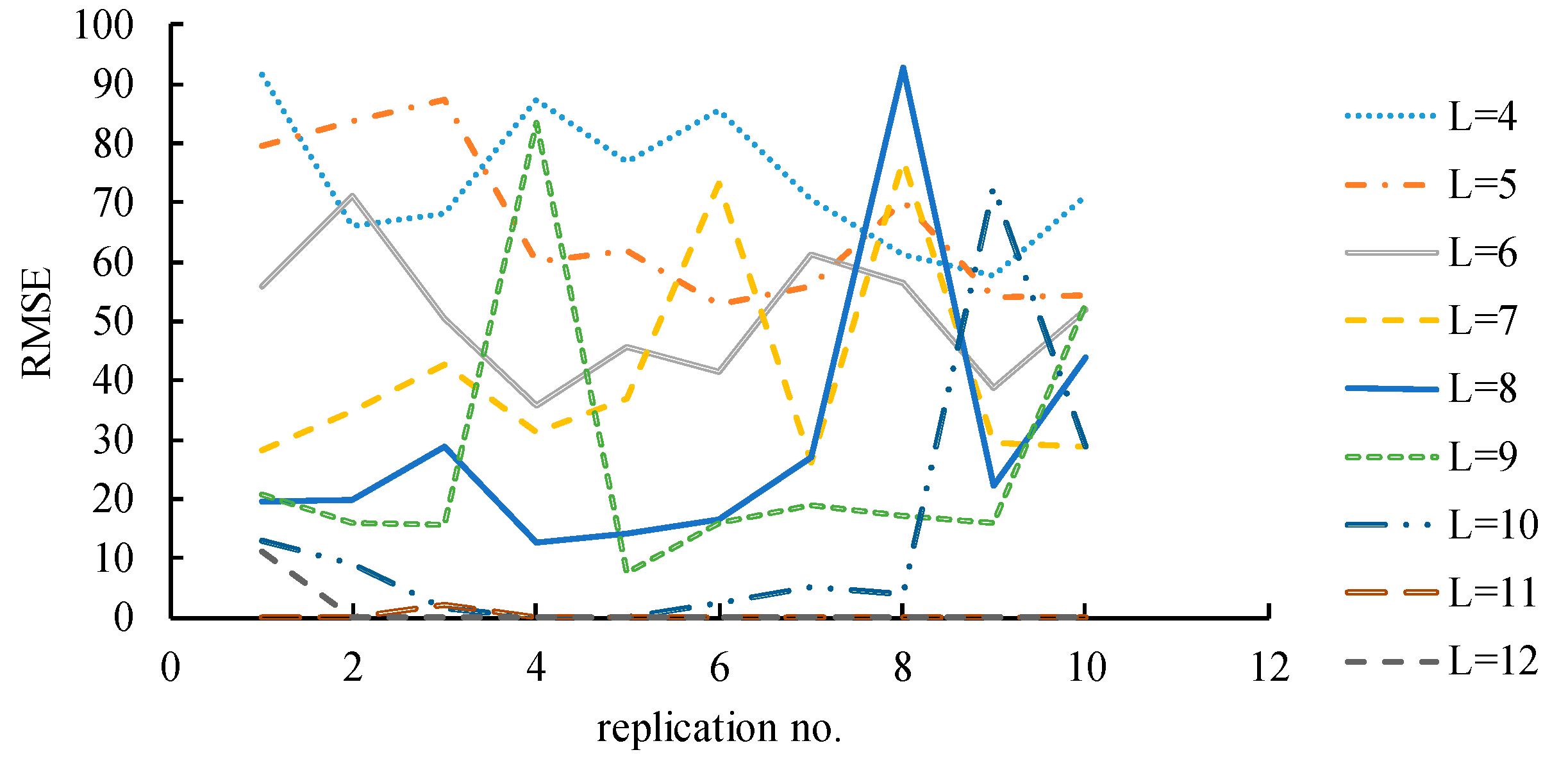
MATLAB was applied to implement the proposed methodology on a PC with an i7-7700 CPU of 3.6 GHz and 8 GB of RAM. First, to derive the cores of the network parameters, SFBPN was treated as a crisp one and was trained using the LM algorithm. To optimize the forecasting accuracy in terms of RMSE, various numbers of nodes in the hidden layer were tried. The results are summarized in Figure 3. With more than eight nodes in the hidden layer, the RMSE for fitting the training data could be reduced to a sufficiently low level (i.e., <30 h). In addition, too many nodes in the hidden layer might increase the possibility of overfitting. Therefore, the number of hidden-layer nodes was set to eight.
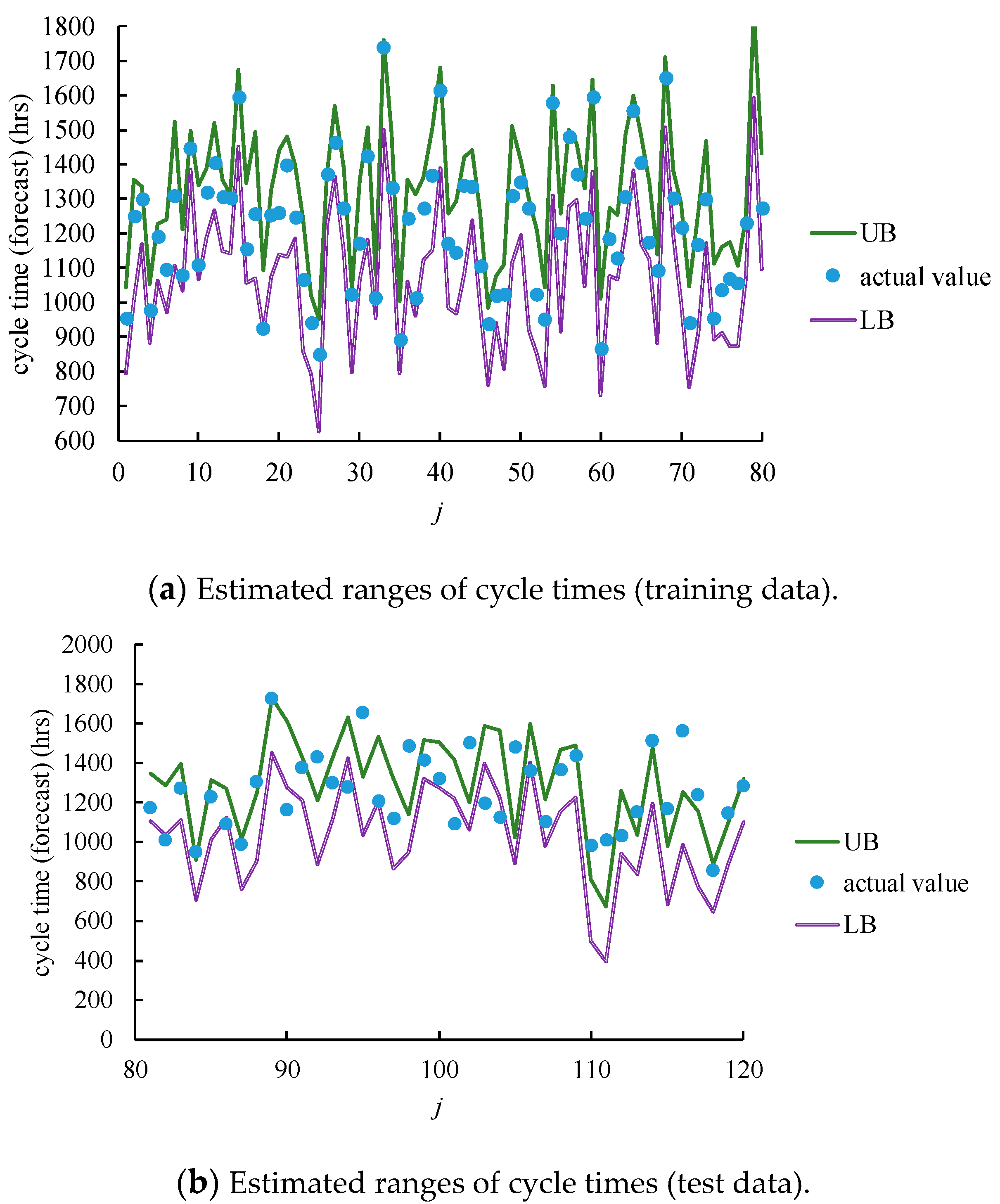
The trained SFBPN was then applied to generate the cores of the fuzzy cycle time forecasts. The results are shown in Figure 4. The SFBPN forecasted the cycle times accurately for the training data. However, some cycle time forecasts deviated from the actual values when the SFBPN was applied to the test data, showing the necessity for estimating the range of a cycle time.
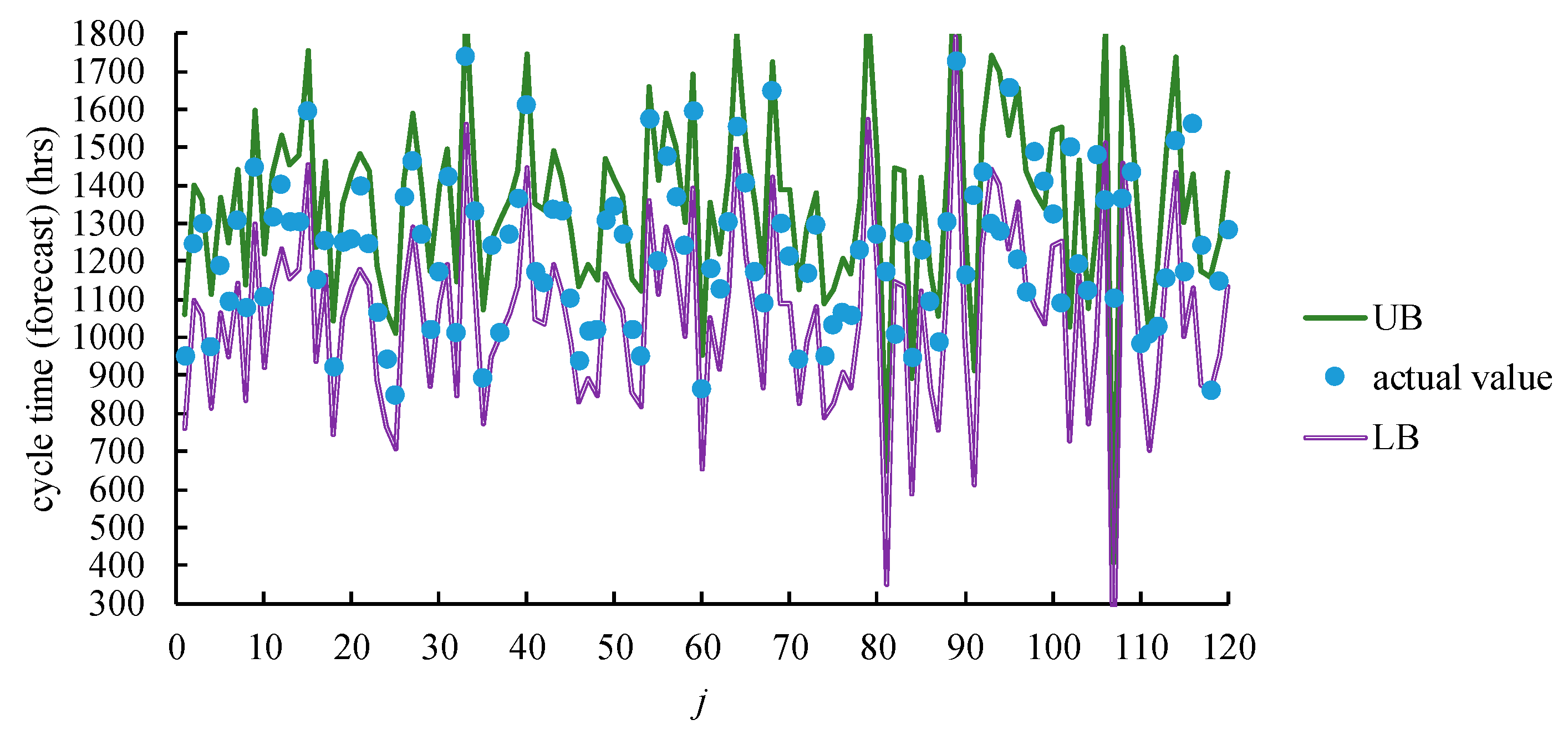
Subsequently, the random search and local optimization algorithm was applied to estimate the range of time by fuzzifying the thresholds on the hidden and output layers. The number of iterations (T) was set to 100. The ranges of random numbers ξ l and ζ l were set to be within [0, 1], i.e., v = 1. The estimation results are shown in Figure 5. For the training data, the estimated range of the cycle time contained the actual value. However, such a property might not hold for test data.
The forecasting precision was evaluated in terms of the average range (AR), hit rate (HR), and the cost for inclusion (CFI):
A R = j = 1 n ( U ( o j 3 ) U ( o j 1 ) ) n
H R = j = 1 n I n ( j ) n 100 %
C F I = A R H R
where
I n ( j ) = { 1 if U ( o j 1 ) a j U ( o j 3 ) 0 otherwise
The results are summarized in Table 3.

4.3. Comparison with Existing Methods

Several existing methods have also been applied to this case for comparison. The first existing method is a traditional statistical analysis technique, the 6σ confidence interval method [26], in which three times the standard deviation was added to and subtracted from the core in order to determine the upper and lower bounds of the cycle time. However, in theory, the probability that a ±3σ confidence interval contains an actual value is only 99.7% under the residual normality assumption. The standard deviation, σ, using the FBPN was derived as follows [1]:
σ = n n P 1 RMSE
In this experiment, σ was 289 h. The forecasting precision using the 6σ confidence interval method is shown in Table 4.
The second existing method is the fuzzy linear regression (FLR)-quadratic programming (QP) method proposed by Donoso et al. [43], in which the relationship between the cycle time of a job and its attributes is fitted with a FLR regression, as follows:
o ˜ j = w ˜ 0 ( + ) p = 1 P w ˜ p x j p
To derive the values of the fuzzy parameters in Equation (69), the following QP problem was solved:
(QP)
Min   Z = ω 1 t = 1 T ( o j 2 a j ) 2 + ω 2 t = 1 T ( o j 3 o j 1 ) 2
subject to
a j o j 1 + s ( o j 2 o j 1 )   1 j n
a j o j 3 + s ( o j 2 o j 3 ) ;   1 j n
o j 1 = w 01 + p = 1 P w p 1 x j p ;   1 j n
o j 2 = w 02 + p = 1 P w p 2 x j p ;   1 j n
o j 3 = w 03 + p = 1 P w p 3 x j p ;   1 j n
w p 1 w p 2 w p 3 ;   0 p P
0 o j 1 o j 2 o j 3 ;   1 j n
where ω 1 and ω 2 are the weights; ω 1 , ω 2 [ 0 ,   1 ] ; ω 1 + ω 2 = 1 . s is the satisfaction level; s [ 0 ,   1 ] . In this study, these parameters were set as ω 1 = 0.3 ; ω 2 = 0.7 ; s = 0.25 . The forecasting precision achieved by applying the FLR-QP method is shown in Table 5.
The third method is the FBPN method proposed by Chen and Lin [17], in which only the threshold on the output node was fuzzified to estimate the range of the cycle time. The estimated ranges of cycle times are shown in Figure 6. The forecasting precision using Chen and Lin’s FBPN method was evaluated, and the results are shown in Table 6.
From the experimental results, the following discussion was made:
(1)
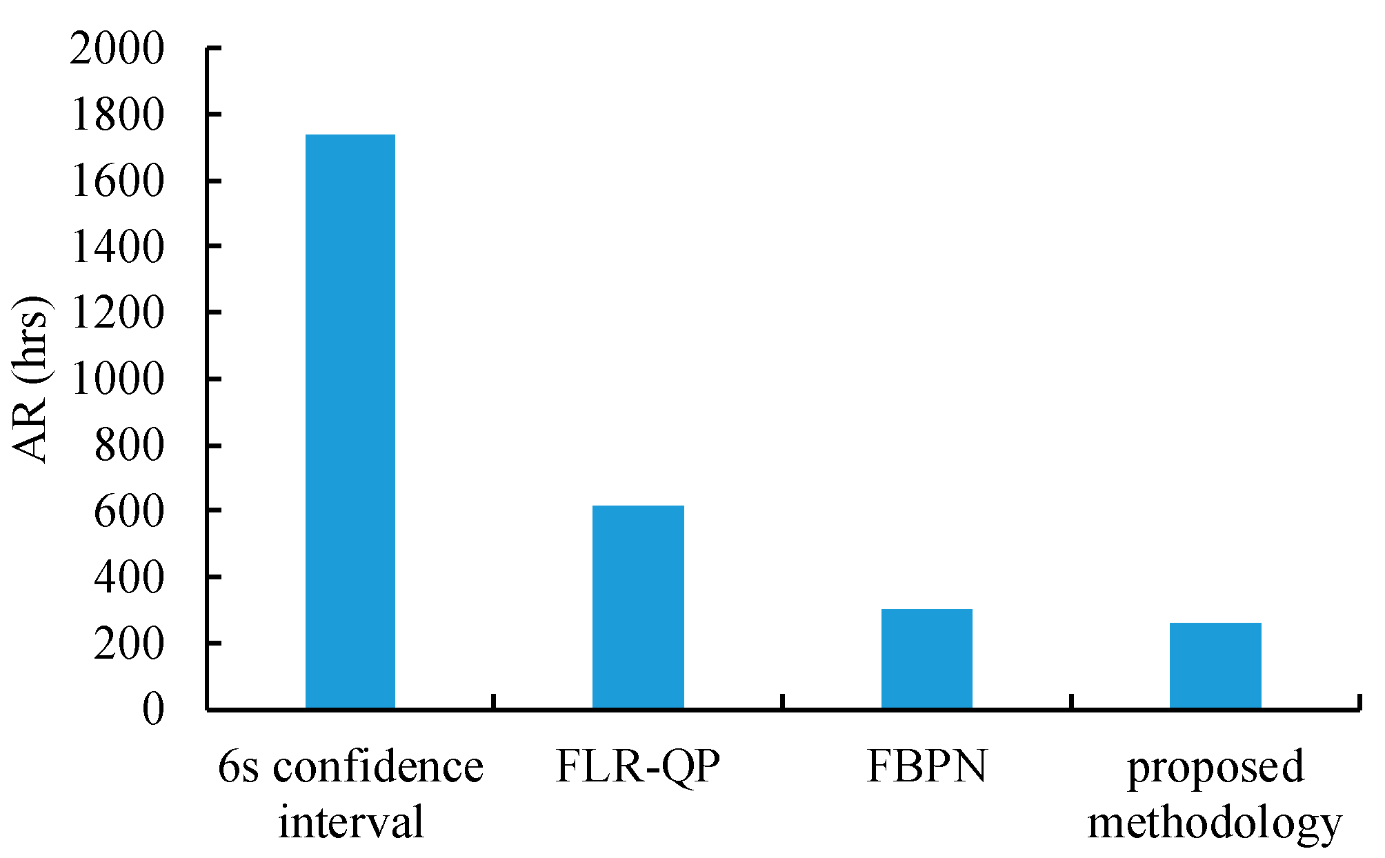
All of the compared methods maximized the hit rate for the training data. However, the average ranges achieved using these methods differed significantly, as illustrated by Figure 7. In this regard, the proposed methodology outperformed the existing methods by establishing the narrowest range for the cycle time.
(2)
It is questionable whether the advantage of the SFBPN approach over the existing methods is significant. To investigate this, the following hypotheses were tested:
Hypothesis 1 (H1).
The estimation precision using the SFBPN approach in terms of the average range is the same as that using the existing method.
Hypothesis 2 (H2).
The estimation precision using the SFBPN approach in terms of the average range is more effective than that using the existing method.
Table 7 presents a summary of the paired t test results. The estimation precision using the SFBPN approach was significantly improved (α = 0.05) when compared with the existing methods.
(3)
For the test data, none of these methods optimized the hit rate and the average range simultaneously. Hit rate was usually enhanced at the expense of wide ranges of fuzzy cycle time forecasts. For this sake, CFI might be a better measure for forecasting precision. In this regard, the proposed methodology surpassed the existing methods through reducing the CFI by up to 65%, as shown in Figure 8.
(4)
In the random search and local optimization algorithm, it is interesting to know whether the ranges of random numbers affected the forecasting performance of the proposed methodology. To investigate this issue, various ranges of ξ l and ζ l were tried so as to observe changes in the forecasting precision. The results are summarized in Figure 9. Obviously, with a wider range, it became more difficult to find the optimal solution, which led to a poorer forecasting precision.

5. Conclusions and Future Research Directions

Forecasting the cycle time of a job is a critical task for a factory. However, owing to the uncertainty of the cycle time, it becomes a challenging task, even with state-of-the-art deep learning techniques. To address this challenge, estimating the range of the cycle time requires a viable treatment. In this study, a SFBPN approach is proposed. In the proposed methodology, thresholds on both the hidden and output layers of a BPN are fuzzified to estimate the range of the cycle time, while in the existing methods, only the threshold on the output node is fuzzified. In this way, the SFBPN approach can further tighten the range of the cycle time. To derive the optimal values of the fuzzy thresholds, a random search and local optimization algorithm is also proposed.
A real case from the literature is adopted to assess the effectiveness of the proposed methodology and to compare it with those of several existing methods. According to the experimental results, the following conclusions were drawn:
(1)
For training data (i.e., learned examples), all of the compared methods were able to include the actual values in the corresponding fuzzy cycle time forecasts or cycle time confidence intervals. However, only the proposed methodology could minimize the average ranges of the fuzzy cycle time forecasts.
(2)
For the test data (i.e., unlearned examples), CFI was a better measure for the forecasting precision. In this regard, the advantage of the proposed methodology over existing methods was up to 65%.
However, the proposed methodology is subject to the following limitations:
(1)
Although the random search and local optimization algorithm is likely to find a promising solution within a short time, it cannot guarantee the global optimality of the solution.
(2)
The case used to illustrate the proposed methodology is relatively small. A larger case needs to be analyzed to further elaborate the effectiveness of the proposed methodology.
In future studies, connection weights in the SFBPN can also be fuzzified to further enhance the forecasting precision; however, this is computationally intense and requires an efficient algorithm [44,45,46]. As an alternative, fuzzifying some thresholds and some connection weights may be more tractable. In addition, the SFBPN approach is a general methodology that can be applied to estimate a range of data with uncertainty in other fields. Furthermore, other types of fuzzy numbers [47] can also be adopted to represent fuzzy thresholds. Hybridizing various methods to achieve total synergy [48] is another direction worth investigation.

Author Contributions

All of the authors equally contributed to the writing of this paper. Data curation, methodology, and writing original draft: T.C., Y.-C.W. and H.-R.T.; writing—review and editing: T.C. and Y.-C.W. All authors have read and agreed to the published version of the manuscript.

Funding

This study was partly funded by Ministry of Science and Technology, Taiwan.

Institutional Review Board Statement

Not applicable.

Informed Consent Statement

Not applicable.

Data Availability Statement

Data is contained within the article.

Acknowledgments

This work was supported by ministry of science of technology of Taiwan.

Conflicts of Interest

The authors declare no conflict of interest.

References

  1. Baykasoğlu, A.; Göçken, M.; Unutmaz, Z.D. New approaches to due date assignment in job shops. Eur. J. Oper. Res. 2008, 187, 31–45. [Google Scholar] [CrossRef]
  2. Öztürk, A.; Kayalıgil, S.; Özdemirel, N.E. Manufacturing lead time estimation using data mining. Eur. J. Oper. Res. 2006, 173, 683–700. [Google Scholar] [CrossRef]
  3. Chang, P.C.; Liao, T.W. Combining SOM and fuzzy rule base for flow time prediction in semiconductor manufacturing factory. Appl. Soft Comput. 2006, 6, 198–206. [Google Scholar] [CrossRef]
  4. Chen, T. An efficient and effective fuzzy collaborative intelligence approach for cycle time estimation in wafer fabrication. Int. J. Intell. Syst. 2015, 30, 620–650. [Google Scholar] [CrossRef]
  5. Vinod, V.; Sridharan, R. Simulation modeling and analysis of due-date assignment methods and scheduling decision rules in a dynamic job shop production system. Int. J. Prod. Econ. 2011, 129, 127–146. [Google Scholar] [CrossRef]
  6. Shabtay, D. Scheduling and due date assignment to minimize earliness, tardiness, holding, due date assignment and batch delivery costs. Int. J. Prod. Econ. 2010, 123, 235–242. [Google Scholar] [CrossRef]
  7. Yin, Y.; Cheng, T.C.E.; Xu, D.; Wu, C.C. Common due date assignment and scheduling with a rate-modifying activity to minimize the due date, earliness, tardiness, holding, and batch delivery cost. Comput. Ind. Eng. 2012, 63, 223–234. [Google Scholar] [CrossRef]
  8. Tirkel, I. The effectiveness of variability reduction in decreasing wafer fabrication cycle time. In Proceedings of the 2013 Winter Simulations Conference, Washington, DC, USA, 8–11 December 2013; pp. 3796–3805. [Google Scholar]
  9. Asadzadeh, S.M.; Azadeh, A.; Ziaeifar, A. A neuro-fuzzy-regression algorithm for improved prediction of manufacturing lead time with machine breakdowns. Concurr. Eng. 2011, 19, 269–281. [Google Scholar] [CrossRef]
  10. Seidel, G.; Lee, C.F.; Tang, A.Y.; Low, S.L.; Gan, B.P.; Scholl, W. Challenges associated with realization of lot level fab out forecast in a giga wafer fabrication plant. In Proceedings of the 2020 Winter Simulation Conference, Orlando, FL, USA, 14–18 December 2020; pp. 1777–1788. [Google Scholar]
  11. Azadeh, A.; Ziaeifar, A.; Pichka, K.; Asadzadeh, S.M. An intelligent algorithm for optimum forecasting of manufacturing lead times in fuzzy and crisp environments. Int. J. Logist. Manag. 2013, 16, 186–210. [Google Scholar] [CrossRef]
  12. Malik, A.I.; Sarkar, B. Coordinating supply-chain management under stochastic fuzzy environment and lead-time reduction. Mathematics 2019, 7, 480. [Google Scholar] [CrossRef] [Green Version]
  13. Chen, T.; Wang, Y.C. Incorporating the FCM–BPN approach with nonlinear programming for internal due date assignment in a wafer fabrication plant. Robot. Comput. Integr. Manuf. 2010, 26, 83–91. [Google Scholar] [CrossRef]
  14. Wang, J.; Zhang, J. Big data analytics for forecasting cycle time in semiconductor wafer fabrication system. Int. J. Prod. Res. 2016, 54, 7231–7244. [Google Scholar] [CrossRef]
  15. Tan, X.; Xing, L.; Cai, Z.; Wang, G. Analysis of production cycle-time distribution with a big-data approach. J. Intell. Manuf. 2020, 31, 1889–1897. [Google Scholar] [CrossRef]
  16. Chen, T.; Wu, H.C. A new cloud computing method for establishing asymmetric cycle time intervals in a wafer fabrication factory. J. Intell. Manuf. 2017, 28, 1095–1107. [Google Scholar] [CrossRef] [Green Version]
  17. Chen, T.C.; Lin, Y.C. A collaborative fuzzy-neural approach for internal due date assignment in a wafer fabrication plant. Int. J. Innov. Comput. Inf. Control. 2011, 7, 5193–5210. [Google Scholar]
  18. Hsieh, L.Y.; Chang, K.H.; Chien, C.F. Efficient development of cycle time response surfaces using progressive simulation metamodeling. Int. J. Prod. Res. 2014, 52, 3097–3109. [Google Scholar] [CrossRef]
  19. Chang, P.C.; Wang, Y.W.; Liu, C.H. Combining SOM and GA-CBR for flow time prediction in semiconductor manufacturing factory. In Proceedings of the International Conference on Rough Sets and Current Trends in Computing, Kobe, Japan, 6–8 November 2006; pp. 767–775. [Google Scholar]
  20. Chen, T. Asymmetric cycle time bounding in semiconductor manufacturing: An efficient and effective back-propagation-network-based method. Oper. Res. 2016, 16, 445–468. [Google Scholar] [CrossRef]
  21. Wang, J.; Zhang, J.; Wang, X. Bilateral LSTM: A two-dimensional long short-term memory model with multiply memory units for short-term cycle time forecasting in re-entrant manufacturing systems. IEEE Trans. Industr. Inform. 2017, 14, 748–758. [Google Scholar] [CrossRef]
  22. Goodfellow, I.; Bengio, Y.; Courville, A.; Bengio, Y. Deep Learning; MIT Press: Cambridge, MA, USA, 2016. [Google Scholar]
  23. Montavon, G.; Samek, W.; Müller, K.R. Methods for interpreting and understanding deep neural networks. Digit Signal Process. 2018, 73, 1–15. [Google Scholar] [CrossRef]
  24. Wang, J.; Zhang, J.; Wang, X. A data driven cycle time prediction with feature selection in a semiconductor wafer fabrication system. IEEE Trans. Semicond. Manuf. 2018, 31, 173–182. [Google Scholar] [CrossRef]
  25. Kuo, P.H.; Huang, C.J. A high precision artificial neural networks model for short-term energy load forecasting. Energies 2018, 11, 213. [Google Scholar] [CrossRef] [Green Version]
  26. Valles, A.; Sanchez, J.; Noriega, S.; Nuñez, B.G. Implementation of Six Sigma in a manufacturing process: A case study. Int. J. Ind. Eng. 2009, 16, 171–181. [Google Scholar]
  27. Gani, A.N.; Assarudeen, S.M. A new operation on triangular fuzzy number for solving fuzzy linear programming problem. Appl. Math. Sci. 2012, 6, 525–532. [Google Scholar]
  28. Wang, J.; Ding, D.; Liu, O.; Li, M. A synthetic method for knowledge management performance evaluation based on triangular fuzzy number and group support systems. Appl. Soft Comput. 2016, 39, 11–20. [Google Scholar] [CrossRef]
  29. Wu, C.L.; Chau, K.W.; Fan, C. Prediction of rainfall time series using modular artificial neural networks coupled with data-preprocessing techniques. J. Hydrol. 2010, 389, 146–167. [Google Scholar] [CrossRef] [Green Version]
  30. Chang, P.-C.; Hsieh, J.-C. A neural networks approach for due-date assignment in a wafer fabrication factory. Eur. J. Ind. Eng. 2003, 10, 55–61. [Google Scholar]
  31. Martino, J.P. A review of selected recent advances in technological forecasting. Technol. Forecast. Soc. Chang. 2003, 70, 719–733. [Google Scholar] [CrossRef]
  32. Tirkel, I. Forecasting flow time in semiconductor manufacturing using knowledge discovery in databases. Int. J. Prod. Res. 2013, 51, 5536–5548. [Google Scholar] [CrossRef]
  33. Chiu, C.; Chang, P.C.; Chiu, N.H. A case-based expert support system for due-date assignment in a wafer fabrication factory. J. Intell. Manuf. 2003, 14, 287–296. [Google Scholar] [CrossRef]
  34. Chan, K.Y.; Kwong, C.K.; Dillon, T.S.; Tsim, Y.C. Reducing overfitting in manufacturing process modeling using a backward elimination based genetic programming. Appl. Soft Comput. 2011, 11, 1648–1656. [Google Scholar] [CrossRef]
  35. Chang, P.C.; Wang, Y.W.; Ting, C.J. A fuzzy neural network for the flow time estimation in a semiconductor manufacturing factory. Int. J. Prod. Res. 2008, 46, 1017–1029. [Google Scholar] [CrossRef]
  36. Wang, J.; Yang, J.; Zhang, J.; Wang, X.; Zhang, W. Big data driven cycle time parallel prediction for production planning in wafer manufacturing. Enterp. Inf. Syst. 2018, 12, 714–732. [Google Scholar] [CrossRef]
  37. Wang, J.; Zheng, P.; Zhang, J. Big data analytics for cycle time related feature selection in the semiconductor wafer fabrication system. Comput. Ind. Eng. 2020, 143, 106362. [Google Scholar] [CrossRef]
  38. Hanss, M. Applied Fuzzy Arithmetic; Springer: Berlin/Heidelberg, Germany, 2005. [Google Scholar]
  39. Yu, W.; Li, X. Fuzzy identification using fuzzy neural networks with stable learning algorithms. IEEE Trans. Fuzzy Syst. 2004, 12, 411–420. [Google Scholar] [CrossRef]
  40. Bonnans, J.F.; Gilbert, J.C.; Lemaréchal, C.; Sagastizábal, C.A. Numerical Optimization: Theoretical and Practical Aspects; Springer Science & Business Media: Berlin, Germany, 2006. [Google Scholar]
  41. Lapedus, M. Battling Fab Cycle Times. Available online: https://semiengineering.com/battling-fab-cycle-times/ (accessed on 16 February 2017).
  42. Hung, Y.F.; Chang, C.B. Dispatching rules using flow time predictions for semiconductor wafer fabrications. J. Chin. Inst. Ind Eng. 2002, 19, 67–75. [Google Scholar] [CrossRef]
  43. Donoso, S.; Marin, N.; Vila, M.A. Quadratic programming models for fuzzy regression. In Proceedings of the International Conference on Mathematical and Statistical Modeling in Honor of Enrique Castillo, Ciudad Real, Spain, 28–30 June 2006. [Google Scholar]
  44. Nauck, D.; Kruse, R. A fuzzy neural network learning fuzzy control rules and membership functions by fuzzy error backpropagation. In Proceedings of the IEEE International Conference on Neural Networks, San Francisco, CA, USA, 28 March–1 April 1993; pp. 1022–1027. [Google Scholar]
  45. Ishibuchi, H.; Kwon, K.; Tanaka, H. A learning algorithm of fuzzy neural networks with triangular fuzzy weights. Fuzzy Sets Syst. 1995, 71, 277–293. [Google Scholar] [CrossRef]
  46. He, W.; Dong, Y. Adaptive fuzzy neural network control for a constrained robot using impedance learning. IEEE Trans. Neural Netw. Learn. Syst. 2017, 29, 1174–1186. [Google Scholar] [CrossRef]
  47. Pamucar, D.; Ecer, F.; Deveci, M. Assessment of alternative fuel vehicles for sustainable road transportation of United States using integrated fuzzy FUCOM and neutrosophic fuzzy MARCOS methodology. Sci. Total Environ. 2021, 788, 147763. [Google Scholar] [CrossRef] [PubMed]
  48. Deveci, M.; Pamucar, D.; Gokasar, I. Fuzzy Power Heronian function based CoCoSo method for the advantage prioritization of autonomous vehicles in real-time traffic management. Sustain. Cities Soc. 2021, 69, 102846. [Google Scholar] [CrossRef]
Figure 1. The implementation procedure of the proposed methodology.
Mathematics 09 01430 g001
Figure 2. The architecture of the selectively fuzzified backpropagation network (SFBPN).
Mathematics 09 01430 g002
Figure 3. RMSEs associated with various numbers of hidden-layer nodes.
Mathematics 09 01430 g003
Figure 4. The cores of fuzzy cycle time forecasts.
Mathematics 09 01430 g004
Figure 5. Estimated ranges of cycle times.
Mathematics 09 01430 g005
Figure 6. Estimated ranges of the cycle times using Chen and Lin’s FBPN method.
Mathematics 09 01430 g006
Figure 7. Average ranges achieved using various methods for the training data.
Mathematics 09 01430 g007
Figure 8. Cost for inclusions (CFIs) using various methods for the test data.
Mathematics 09 01430 g008
Figure 9. Effect of the range of random numbers on the average range of fuzzy cycle time forecasts.
Mathematics 09 01430 g009
Table 1. The novelty of the proposed methodology.
MethodType of Cycle Time ForecastsFuzzified ParametersOptimization MethodPrecision
Wang and Zhang [14]CrispNoOptimized feature selectionLow
Chen and Wu [16]FuzzyThreshold on the node of the output layerEquations based on the linear function of the outputHigh
Wang et al. [21]CrispNoDeep learningLow
Wang et al. [24]CrispNoOptimized feature selectionLow−moderate
The proposed methodologyFuzzyThresholds on nodes of hidden and output layersRandom search and local optimization algorithmVery high
Table 2. Factors influential to the cycle time of a job.
VariableDefinition
x j 1 job size (pieces)
x j 2 fab work-in-process (WIP; jobs)
x j 3 queue length before the bottleneck (jobs)
x j 4 queue length on the processing route (jobs)
x j 5 average waiting time of recently completed jobs (h)
x j 6 fab utilization
Table 3. The forecasting precision achieved using the proposed methodology.
Data PartAR (h)HRCFI (h)
Training260100%260
Test26143%613
Table 4. The forecasting precision using the 6σ confidence interval method.
Data PartAR (h)HRCFI (h)
Training1736100%1736
Test1736100%1736
Table 5. The forecasting precision achieved by applying the FLR-QP method.
Data PartAR (h)HRCFI (h)
Training617100%617
Test616100%616
Table 6. The forecasting precision using the FBPN method proposed by Chen and Lin [17].
Data PartAR (h)HRCFI (h)
Training301100%301
Test30143%709
Table 7. The paired t test results.
6σ Confidence IntervalFLR-QPFBPNSFBPN
Mean1736.5616.8301.1260.0
Variation6.4 × 10−24506.677.64856.5
Observations80808080
Pearson correlation coefficient0.005−0.091−0.168
Degree of freedom797979
t statistic189.542.465.12
P(Tt) one-tail4.4 × 10−1071.87 × 10−561.07 × 10⁻⁶
t Critical one-tail1.661.661.66
P(Tt) two-tail8.7 × 10−1073.74 × 10−562.14 × 10⁻⁶
t Critical two-tail1.991.991.99
Publisher’s Note: MDPI stays neutral with regard to jurisdictional claims in published maps and institutional affiliations.