
A Robust Approach for Identifying the Major Components of the Bribery Tolerance Index


Abstract
:1. Introduction
2. Materials and Methods
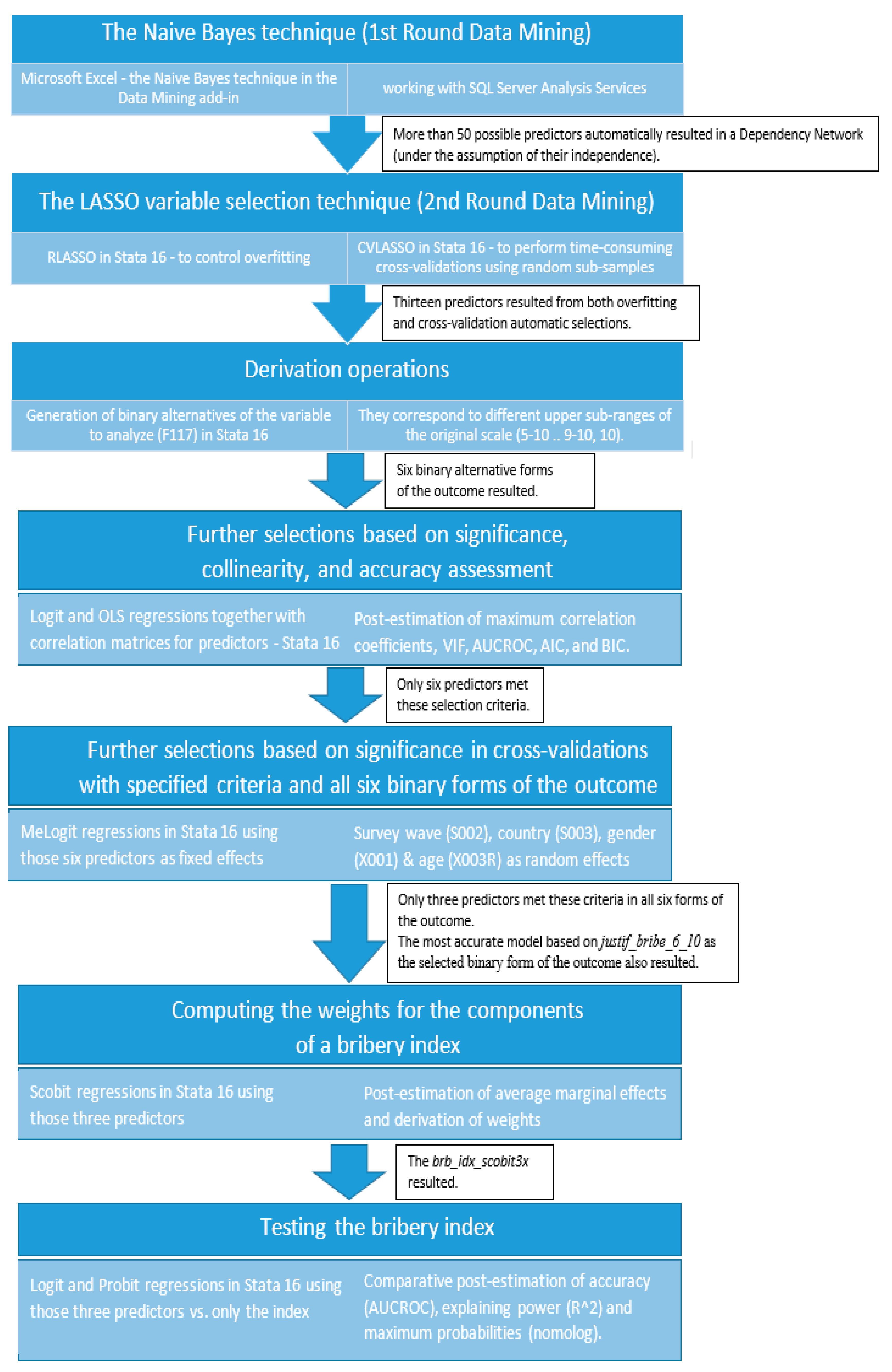
- The Naive Bayes algorithm in the Microsoft Data Mining (DM) add-in available in Microsoft Excel and working with SQL Server Analysis Services 2016 Enterprise Edition x64 (SSAS) which acted as first-round mining (maximum ~10.7 GB of RAM (Random Access Memory) consumed only by SSAS and maximum ~5.3 additionally used by Excel on a Windows Server 2016 Datacenter virtual machine with six Intel Xeon Gold 6240 Cascadelake CPU cores and 24.4 GB of RAM (maximum ~18.5 GB consumed including the operating system) running on one of the private clouds (https://cloud.raas.uaic.ro/; https://tinyurl.com/4wn9huwj—last accessed on 9 June 2021) of Alexandru Ioan Cuza University, currently managed using OpenStack on Ubuntu and dedicated to research;
- Two forms of LASSO, originally documented in geophysics as an L1-regularization approach for a problem called sparse spike deconvolution [21,22,23], namely RLASSO (rigorous and penalizing LASSO to control overfitting), and CVLASSO (the LASSO which performs time-consuming cross-validation—here with the LSE option = largest lambda for which the Means Squared Prediction Error-MSPE is within one standard error of the minimal MSPE) in Stata 16 MP-64 bit (second round mining);
- Cross-validations using the mixed-effects technique (melogit—variables to select from as fixed effects) and checks of significance loss using the value of p—it was additionally considered the significance level of 1‰ starting from the fact that in large samples, p-values tend to decrease quickly to zero [27] when considering six binary forms (derived also in Stata) of the dependent variable (F117—Table 1 and Table 2) and four criteria (random effects): wave, country, sex, and age;
- Smaller values of AIC-Akaike Information Criterion, and BIC-Bayesian Information Criterion [28] for a better fit of the chosen model [29], where the goodness of fit describes how well a statistical model fits a set of observations; larger ones for both p (contradiction of the Ho hypothesis) in the case of GOF (Goodness of Fit) test and chi2 for the same GOF as additional indications of a better fit of the model; and
- Larger R-squared [30] for a better explaining power of the models.
- p is the probability (risk) of bribery tolerance;
- (1 − p) is the probability of not considering bribes acceptable;
- p/(1 − p) represents the odds of bribery tolerance;
- i = 2, …, n and n is the total number of independent variables;
- β0 is the bias (intercept) term;
- βi measures the effect of a change in variable Xi on the risk of bribery tolerance;
- Xi is one explanatory variable from the array (∑) of features selected after using LASSO; and
- ε represents the error term.
3. Results
4. Discussion and Conclusions
Author Contributions
Funding
Institutional Review Board Statement
Informed Consent Statement
Data Availability Statement
Acknowledgments
Conflicts of Interest
Appendix A
References
- King, G. Ensuring the data-rich future of the social sciences. Science 2011, 331, 719–721. [Google Scholar] [CrossRef]
- Einav, L.; Levin, J. Economics in the age of big data. Science 2014, 346, 1243089. [Google Scholar] [CrossRef]
- Booysen, F. An overview and evaluation of composite indices of development. Soc. Indic. Res. 2002, 59, 115–151. [Google Scholar] [CrossRef]
- De Muro, P.; Mazziotta, M.; Pareto, A. Composite indices of development and poverty: An application to MDGs. Soc. Indic. Res. 2011, 104, 1–18. [Google Scholar] [CrossRef]
- Shaker, R.R.; Zubalsky, S.L. Examining patterns of sustainability across Europe: A multivariate and spatial assessment of 25 composite indices. Int. J. Sustain. Dev. World Ecol. 2015, 22, 1–13. [Google Scholar] [CrossRef]
- Horodnic, I.A.; Williams, C.C.; Ianole-Calin, R. Does higher cash-in-hand income motivate young people to engage in under-declared employment? East. J. Eur. Stud. 2020, 11, 48–69. [Google Scholar]
- Turturean, C.I.; Asandului, L.A.; Chirila, C.; Homocianu, D. Composite index of sustainable development of EU countries’economies (ISDE-EU). Transform. Bus. Econ. 2019, 18, 586–605. [Google Scholar]
- Yoneoka, D.; Saito, E.; Nakaoka, S. New algorithm for constructing area-based index with geographical heterogeneities and variable selection: An application to gastric cancer screening. Sci. Rep. 2016, 6, 26582. [Google Scholar] [CrossRef] [PubMed] [Green Version]
- Druică, E.; Vâlsan, C.; Ianole-Călin, R.; Mihail-Papuc, R.; Munteanu, I. Exploring the Link between Academic Dishonesty and Economic Delinquency: A Partial Least Squares Path Modeling Approach. Mathematics 2019, 7, 1241. [Google Scholar] [CrossRef] [Green Version]
- Wheeler, D.C. Simultaneous coefficient penalization and model selection in geographically weighted regression: The geographically weighted lasso. Environ. Plan. 2009, 41, 722–742. [Google Scholar] [CrossRef] [Green Version]
- Nakaya, T. Evaluating socioeconomic inequalities in cancer mortality by using areal statistics in Japan: A note on the relation between the municipal cancer mortality and the areal deprivation index. Proc. Inst. Stat. Math. 2011, 59, 239–265. [Google Scholar]
- Hindman, M. Building better models: Prediction, replication, and machine learning in the social sciences. Ann. Am. Acad. Political Soc. Sci. 2015, 659, 48–62. [Google Scholar] [CrossRef]
- Requejo-Castro, D.; Giné-Garriga, R.; Pérez-Foguet, A. Data-driven Bayesian network modelling to explore the relationships between SDG 6 and the 2030 Agenda. Sci. Total. Environ. 2020, 710, 136014. [Google Scholar] [CrossRef]
- Imani, M.; Ghoreishi, S.F. Two-Stage Bayesian Optimization for Scalable Inference in State-Space Models. IEEE Trans. Neural Netw. Learn. Syst. 2021. [Google Scholar] [CrossRef] [PubMed]
- Dixon, M.F.; Halperin, I.; Bilokon, P. Machine Learning in Finance. From Theory to Practice; Springer Nature: Cham, Switzerland, 2020. [Google Scholar] [CrossRef]
- Chabova, K. Measuring corruption in Europe: Public opinion surveys and composite indices. Qual. Quant. 2017, 51, 1877–1900. [Google Scholar] [CrossRef]
- Fazekas, M.; Tóth, I.J.; King, L.P. Anatomy of grand corruption: A composite corruption risk index based on objective data. In Corruption Research Center Budapest Working Papers No. CRCB-WP/2013, 2; Institute of Economics, Centre for Economic and Regional Studies: Budapest, Hungary, 2013. [Google Scholar]
- Villarino, J.M.B. Measuring corruption: A critical analysis of the existing datasets and their suitability for diachronic transnational research. Soc. Indic. Res. 2021, 1–39. [Google Scholar] [CrossRef]
- Dobrowolski, Z. Combating Corruption and Other Organizational Pathologies; Peter Lang: Frankfurt Am Main, Germany, 2016; pp. 100–106. [Google Scholar] [CrossRef]
- Lambsdorff, J.G. The Methodology of the Corruption Perceptions Index 2007. Internet Center for Corruption Research. 2007. Available online: http://www.icgg.org/corruption.cpi_2006.html (accessed on 1 June 2021).
- Levy, S.; Fullagar, P.K. Reconstruction of a sparse spike train from a portion of its spectrum and application to high-resolution deconvolution. Geophysics 1981, 46, 1235–1243. [Google Scholar] [CrossRef]
- Santosa, F.; Symes, W.W. Linear Inversion of Band-Limited Reflection Seismograms. SIAM J. Sci. Stat. Comput. 1986, 7, 1307–1330. [Google Scholar] [CrossRef]
- Tibshirani, R. Regression shrinkage and selection via the lasso. J. R. Stat. Society. Ser. B 1996, 58, 267–288. [Google Scholar] [CrossRef]
- Mukaka, M. A guide to appropriate use of correlation coefficient in medical research. Malawi Med. J. 2012, 24, 69–71. [Google Scholar] [PubMed]
- Jiménez-Valverde, A. Insights into the area under the receiver operating characteristic curve (AUC) as a discrimination measure in species distribution modelling. Glob. Ecol. Biogeogr. 2012, 21, 498–507. [Google Scholar] [CrossRef]
- Bewick, V.; Cheek, L.; Ball, J. Review. Statistics review 14: Logistic regression. Crit. Care 2005, 9, 112–118. [Google Scholar] [CrossRef] [Green Version]
- Lin, M.; Lucas, H.; Shmueli, G. Too big to fail: Large samples and the p-value problem. Inf. Syst. Res. 2013, 24, 906–917. [Google Scholar] [CrossRef] [Green Version]
- Dziak, J.J.; Coffman, D.L.; Lanza, S.T.; Li, R.; Jermiin, L.S. Sensitivity and Specificity of Information Criteria. Brief. Bioinform. 2020, 21, 553–565. [Google Scholar] [CrossRef]
- Kéry, M.; Royle, J.A. Modeling Static Occurrence and Species Distributions Using Siteoccupancy Models. Appl. Hierarchical Modeling Ecol. 2016, 551–629. [Google Scholar] [CrossRef]
- Miles, J.R. Squared, adjusted r squared. In Encyclopedia of Statistics in Behavioral Science; Wiley: New York, NY, USA, 2005. [Google Scholar] [CrossRef]
- Nagler, J. An alternative estimator to Logit and Probit. Am. J. Political Sci. 1994, 38, 230–255. [Google Scholar] [CrossRef]
- Zlotnik, A.; Abraira, V. A general-purpose nomogram generator for predictive logistic regression models. Stata J. 2015, 15, 537–546. [Google Scholar] [CrossRef] [Green Version]
- Yao, Z.; Holmbom, A.H.; Eklund, T.; Back, B. Combining Unsupervised and Supervised Data Mining Techniques for Conducting Customer Portfolio Analysis. In Advances in Data Mining. Applications and Theoretical Aspects; Perner, P., Ed.; ICDM 2010. Lecture Notes in Computer Science; Springer: Berlin/Heidelberg, Germany, 2010; Volume 6171. [Google Scholar] [CrossRef]
- Vatcheva, K.P.; Lee, M.J.; McCormick, J.B.; Rahbar, M.H. Multi-collinearity in Regression Analyses Conducted in Epidemiologic Studies. Epidemiology 2016, 6, 227. [Google Scholar] [PubMed] [Green Version]
- Shrestha, N. Detecting Multicollinearity in Regression Analysis. Am. J. Appl. Math. Stat. 2020, 8, 39–42. [Google Scholar] [CrossRef]
- Freund, R.J.; Wilson, W.J.; Sa, P. Regression Analysis: Statistical Modeling of a Response Variable, 2nd ed.; Academic Press: Cambridge, MA, USA, 2006. [Google Scholar]
- Ten Have, T.R.; Kunselman, A.R.; Tran, L. A comparison of mixed effects logistic regression models for binary response data with two nested levels of clustering. Stat. Med. 1999, 18, 947–960. [Google Scholar] [CrossRef]
- Horodnic, I.; Rodgers, P.; Williams, C.; Momtazian, L. (Eds.) The Informal Economy: Exploring Drivers and Practices; Routledge: London, UK, 2017. [Google Scholar]
- Vâlsan, C.; Druică, E.; Ianole-Călin, R. State capacity and tolerance towards tax evasion: First evidence from Romania. Adm. Sci. 2020, 10, 33. [Google Scholar] [CrossRef]
- Shafiq, M.N. Aspects of Moral Change in India, 1990–2006: Evidence from Public Attitudes toward Tax Evasion and Bribery. World Dev. 2015, 68, 136–148. [Google Scholar] [CrossRef]
- James, S.; McGee, R.W.; Benk, S.; Budak, T. How seriously do taxpayers regard tax evasion? A survey of opinion in England. J. Money Laund. Control. 2019. Available online: https://www.emerald.com/insight/content/doi/10.1108/JMLC-09-2018-0056/full/html (accessed on 1 June 2021).
- McGee, R.W.; Devos, K.; Benk, S. Attitudes towards tax evasion in Turkey and Australia: A comparative study. Soc. Sci. 2016, 5, 10. [Google Scholar] [CrossRef] [Green Version]
- Aljaaidi, K.S.Y.; Manaf, N.A.A.; Karlinsky, S.S. Tax evasion as a crime: A survey of perception in Yemen. Int. J. Bus. Manag. 2011, 6, 190. [Google Scholar] [CrossRef] [Green Version]
- Munafò, M.R.; Smith, G.D. Robust research needs many lines of evidence. Nature 2018, 553, 399–401. [Google Scholar] [CrossRef] [Green Version]
- Roberts, D.R.; Bahn, V.; Ciuti, S.; Boyce, M.S.; Elith, J.; Guillera-Arroita, G.; Hauenstein, S.; Lahoz-Monfort, J.J.; Schröder, B.; Thuiller, W.; et al. Cross-validation strategies for data with temporal, spatial, hierarchical, or phylogenetic structure. Ecography 2017, 40, 913–929. [Google Scholar] [CrossRef]
- Baker, M. 1500 Scientists Lift the Lid on Reproducibility. Nature 2016, 533, 452–454. [Google Scholar] [CrossRef] [PubMed] [Green Version]


| Variable | Question | Coding |
|---|---|---|
| E290 | Justifiable: Political violence (DK/NA as blanks) | 1–10 scale |
| F114A | Justifiable: Claiming government benefits to which you are not entitled(DK/NA as blanks) | 1–10 scale |
| F114B | Justifiable: Stealing property (DK/NA as blanks) | 1–10 scale |
| F114D | Justifiable: Violence against other people (DK/NA as blanks) | 1–10 scale |
| F114E | Justifiable: Terrorism as a political, ideological, or religious mean(DK/NA as blanks) | 1–10 scale |
| F115 | Justifiable: Avoiding a fare on public transport (DK/NA as blanks) | 1–10 scale |
| F116 | Justifiable: Cheating on taxes (DK/NA as blanks) | 1–10 scale |
| F119 | Justifiable: Prostitution (DK/NA as blanks) | 1–10 scale |
| F199 | Justifiable: For a man to beat his wife (DK/NA as blanks) | 1–10 scale |
| Y010 | SACSECVAL—Welzel Overall Secular Values (DK/NA as blanks) | 0–1 scale |
| F117 (original outcome) | Justifiable: Someone accepting a bribe (DK/NA as blanks) | 1–10 scale |
| justif_bribe_5_10 | 1 if F117 != Blank AND F117 >= 5; 0 if F117 != Blank AND F117 < 5 | 0 or 1 |
| justif_bribe_6_10 | 1 if F117 != Blank AND F117 >= 6; 0 if F117 != Blank AND F117 < 6 AND F117 > 0 | 0 or 1 |
| justif_bribe_7_10 | 1 if F117 != Blank AND F117 >= 7; 0 if F117 != Blank AND F117 < 7 AND F117 > 0 | 0 or 1 |
| justif_bribe_8_10 | 1 if F117 != Blank AND F117 >= 8; 0 if F117 != Blank AND F117 < 8 AND F117 > 0 | 0 or 1 |
| justif_bribe_9_10 | 1 if F117 != Blank AND F117 >= 9; 0 if F117 != Blank AND F117 < 9 AND F117 > 0 | 0 or 1 |
| justif_bribe_10 | 1 if F117 == 10; 0 if F117 != Blank AND F117 < 10 AND F117 > 0 | 0 or 1 |
| Variable | n | Mean | Std.Dev. | Min | 0.25 | Median | 0.75 | Max |
|---|---|---|---|---|---|---|---|---|
| E290 | 67,841 | 1.96 | 1.91 | 1 | 1 | 1 | 2 | 10 |
| F114A | 396,038 | 2.65 | 2.52 | 1 | 1 | 1 | 4 | 10 |
| F114B | 158,481 | 1.8 | 1.8 | 1 | 1 | 1 | 2 | 10 |
| F114D | 158,284 | 1.95 | 1.88 | 1 | 1 | 1 | 2 | 10 |
| F114E | 66,858 | 1.79 | 1.81 | 1 | 1 | 1 | 2 | 10 |
| F115 | 388,305 | 2.6 | 2.45 | 1 | 1 | 1 | 4 | 10 |
| F116 | 394,728 | 2.26 | 2.22 | 1 | 1 | 1 | 3 | 10 |
| F119 | 360,755 | 2.63 | 2.48 | 1 | 1 | 1 | 4 | 10 |
| F199 | 230,248 | 1.94 | 1.99 | 1 | 1 | 1 | 2 | 10 |
| Y010 | 411,064 | 0.35 | 0.18 | 0 | 0.22 | 0.35 | 0.47 | 1 |
| F117 (original outcome) | 410,100 | 1.84 | 1.84 | 1 | 1 | 1 | 2 | 10 |
| justif_bribe_5_10 | 410,100 | 0.09 | 0.29 | 0 | 0 | 0 | 0 | 1 |
| justif_bribe_6_10 | 410,100 | 0.06 | 0.24 | 0 | 0 | 0 | 0 | 1 |
| justif_bribe_7_10 | 410,100 | 0.04 | 0.2 | 0 | 0 | 0 | 0 | 1 |
| justif_bribe_8_10 | 410,100 | 0.03 | 0.17 | 0 | 0 | 0 | 0 | 1 |
| justif_bribe_9_10 | 410,100 | 0.02 | 0.14 | 0 | 0 | 0 | 0 | 1 |
| justif_bribe_10 | 410,100 | 0.02 | 0.12 | 0 | 0 | 0 | 0 | 1 |
| Input Variable/Model | (1) | (2) | (3) | (4) | (5) | (6) | (7) | (8) | (9) |
|---|---|---|---|---|---|---|---|---|---|
| Dependent Variable | justif_bribe_ 5_10 | justif_bribe_ 5_10 | justif_bribe_ 5_10 | justif_bribe_ 6_10 | justif_bribe_ 6_10 | justif_bribe_ 6_10 | justif_bribe_ 7_10 | justif_bribe_ 7_10 | justif_bribe_ 7_10 |
| Model Type | Logit—No Random Effects | MeLogit—Random Effects on Wave (S002) | MeLogit—Random Effects on Country (S003) | Logit—No Random Effects | MeLogit—Random Effects on Wave (S002) | MeLogit—Random Effects on Country (S003) | Logit—No Random Effects | MeLogit—Random Effects on Wave (S002) | MeLogit—Random Effects on Country (S003) |
| F114A | 0.1472 *** | 0.1481 *** | 0.1309 *** | 0.1549 *** | 0.1560 *** | 0.1407 *** | 0.1606 *** | 0.1612 *** | 0.1488 *** |
| (0.0048) | (0.0101) | (0.0130) | (0.0058) | (0.0176) | (0.0147) | (0.0067) | (0.0194) | (0.0203) | |
| F114D | 0.2969 *** | 0.2960 *** | 0.2468 *** | 0.2690 *** | 0.2673 *** | 0.2218 *** | 0.2329 *** | 0.2314 *** | 0.1935 *** |
| (0.0055) | (0.0134) | (0.0209) | (0.0060) | (0.0132) | (0.0211) | (0.0067) | (0.0032) | (0.0215) | |
| F115 | 0.0995 *** | 0.0999 *** | 0.0851 *** | 0.1095 *** | 0.1101 *** | 0.1008 *** | 0.1052 *** | 0.1057 *** | 0.0988 *** |
| (0.0053) | (0.0042) | (0.0140) | (0.0063) | (0.0068) | (0.0116) | (0.0074) | (0.0121) | (0.0129) | |
| F116 | 0.3692 *** | 0.3685 *** | 0.3501 *** | 0.3606 *** | 0.3594 *** | 0.3384 *** | 0.3622 *** | 0.3613 *** | 0.3380 *** |
| (0.0052) | (0.0446) | (0.0265) | (0.0058) | (0.0495) | (0.0243) | (0.0068) | (0.0554) | (0.0266) | |
| F119 | 0.1367 *** | 0.1375 *** | 0.1672 *** | 0.1448 *** | 0.1460 *** | 0.1661 *** | 0.1369 *** | 0.1378 *** | 0.1548 *** |
| (0.0049) | (0.0130) | (0.0157) | (0.0058) | (0.0070) | (0.0150) | (0.0067) | (0.0135) | (0.0179) | |
| Y010 | 1.8602 *** | 1.8565 *** | 2.9867 *** | 0.9335 *** | 0.9239 *** | 1.8382 *** | 0.1470 | 0.1372 * | 1.0877 *** |
| (0.0794) | (0.2581) | (0.2827) | (0.0934) | (0.1112) | (0.2746) | (0.1061) | (0.0697) | (0.2936) | |
| _cons | −6.3675 *** | −6.3686 *** | −6.8198 *** | −6.7649 *** | −6.7639 *** | −7.1348 *** | −6.8293 *** | −6.8259 *** | −7.2325 *** |
| (0.0440) | (0.1273) | (0.1517) | (0.0537) | (0.1819) | (0.1774) | (0.0602) | (0.1926) | (0.1882) | |
| var(_cons[S002]) | N/A | 0.0024 *** | N/A | N/A | 0.0053 *** | N/A | N/A | 0.0033 *** | N/A |
| N/A | (0.0001) | N/A | N/A | (0.0006) | N/A | N/A | (0.0008) | N/A | |
| var(_cons[S003]) | N/A | N/A | 0.3525 *** | N/A | N/A | 0.3266 *** | N/A | N/A | 0.3086 *** |
| N/A | N/A | (0.0730) | N/A | N/A | (0.0641) | N/A | N/A | (0.0701) | |
| N | 122,545 | 122,545 | 122,545 | 122,545 | 122,545 | 122,545 | 122,545 | 122,545 | 122,545 |
| Chi^2 | 18,816.6205 | N/A | 2364.8383 | 15,184.0298 | N/A | 1535.5780 | 12,985.2662 | N/A | 1418.4369 |
| p | 0.0000 | N/A | 0.0000 | 0.0000 | N/A | 0.0000 | 0.0000 | N/A | 0.0000 |
| Pseudo R^2 | 0.4489 | N/A | N/A | 0.4585 | N/A | N/A | 0.4504 | N/A | N/A |
| maxAbsCorCoefPredMtrx | 0.4995 | N/A | N/A | 0.4995 | N/A | N/A | 0.4995 | N/A | N/A |
| AUCROC | 0.9220 | N/A | N/A | 0.9271 | N/A | N/A | 0.9251 | N/A | N/A |
| pGOF | 0.0363 | N/A | N/A | 0.2091 | N/A | N/A | 0.0000 | N/A | N/A |
| Chi^2GOF | 82,080.56 | N/A | N/A | 81,681.32 | N/A | N/A | 83,315.83 | N/A | N/A |
| AIC | 48,401.9455 | 48,379.8688 | 46,746.5493 | 35,258.8082 | 35,228.5612 | 34,194.5529 | 28,095.9260 | 28,077.7890 | 27,351.2618 |
| BIC | 48,469.9591 | 48,399.3012 | 46,824.2792 | 35,326.8219 | 35,247.9937 | 34,272.2828 | 28,163.9396 | 28,097.2215 | 27,428.9916 |
| maxPnomologBiggerThan | 0.9500 | N/A | N/A | 0.9000 | N/A | N/A | 0.9000 | N/A | N/A |
| Input Variable/Model | (1) | (2) | (3) | (4) | (5) | (6) | (7) | (8) | (9) |
|---|---|---|---|---|---|---|---|---|---|
| Dependent Variable | justif_bribe_ 8_10 | justif_bribe_ 8_10 | justif_bribe_ 8_10 | justif_bribe_ 9_10 | justif_bribe_ 9_10 | justif_bribe_ 9_10 | justif_bribe_ 10 | justif_bribe_ 10 | justif_bribe_ 10 |
| Model Type | Logit—No Random Effects | MeLogit—Random Effects on Wave (S002) | MeLogit—Random Effects on Country (S003) | Logit—No Random Effects | MeLogit—Random Effects on Wave (S002) | MeLogit—Random Effects on Country (S003) | Logit—No Random Effects | MeLogit—Random Effects on Wave (S002) | MeLogit—Random Effects on Country (S003) |
| F114A | 0.1617 *** | 0.1620 *** | 0.1528 *** | 0.1683 *** | 0.1685 *** | 0.1603 *** | 0.1743 *** | 0.1743 *** | 0.1677 *** |
| (0.0078) | (0.0153) | (0.0282) | (0.0096) | (0.0256) | (0.0379) | (0.0116) | (0.0386) | (0.0446) | |
| F114D | 0.1953 *** | 0.1941 *** | 0.1628 *** | 0.1728 *** | 0.1712 *** | 0.1456 *** | 0.1491 *** | 0.1489 ** | 0.1376 *** |
| (0.0076) | (0.0097) | (0.0211) | (0.0090) | (0.0273) | (0.0223) | (0.0105) | (0.0469) | (0.0206) | |
| F115 | 0.0987 *** | 0.0990 *** | 0.0985 *** | 0.0899 *** | 0.0902 *** | 0.1003 *** | 0.0756 *** | 0.0756 | 0.1003 *** |
| (0.0087) | (0.0173) | (0.0154) | (0.0106) | (0.0242) | (0.0175) | (0.0125) | (0.0402) | (0.0198) | |
| F116 | 0.3742 *** | 0.3736 *** | 0.3450 *** | 0.3917 *** | 0.3911 *** | 0.3460 *** | 0.4122 *** | 0.4122 *** | 0.3521 *** |
| (0.0084) | (0.0613) | (0.0331) | (0.0108) | (0.0769) | (0.0419) | (0.0136) | (0.0896) | (0.0497) | |
| F119 | 0.1170 *** | 0.1177 *** | 0.1376 *** | 0.0937 *** | 0.0948 | 0.1229 *** | 0.0656 *** | 0.0658 | 0.1058 ** |
| (0.0079) | (0.0304) | (0.0255) | (0.0095) | (0.0529) | (0.0350) | (0.0111) | (0.0660) | (0.0405) | |
| Y010 | −0.5917 *** | −0.6018 *** | 0.4050 | −1.0694 *** | −1.0876 *** | −0.1236 | −1.2979 *** | −1.3014 *** | −0.9532 * |
| (0.1200) | (0.0938) | (0.3318) | (0.1412) | (0.1836) | (0.3513) | (0.1602) | (0.3919) | (0.4145) | |
| _cons | −6.8296 *** | −6.8253 *** | −7.3027 *** | −7.0661 *** | −7.0586 *** | −7.6234 *** | −7.2663 *** | −7.2647 *** | −7.6797 *** |
| (0.0674) | (0.1518) | (0.2112) | (0.0824) | (0.1287) | (0.2835) | (0.0999) | (0.1797) | (0.3525) | |
| var(_cons[S002]) | N/A | 0.0022 * | N/A | N/A | 0.0037 *** | N/A | N/A | 0.0003 | N/A |
| N/A | (0.0009) | N/A | N/A | (0.0010) | N/A | N/A | (0.0005) | N/A | |
| var(_cons[S003]) | N/A | N/A | 0.3415 *** | N/A | N/A | 0.5071 *** | N/A | N/A | 0.5515 *** |
| N/A | N/A | (0.0730) | N/A | N/A | (0.1222) | N/A | N/A | (0.1209) | |
| N | 122,545 | 122,545 | 122,545 | 122,545 | 122,545 | 122,545 | 122,545 | 122,545 | 122,545 |
| Chi^2 | 10,868.6143 | N/A | 1163.2037 | 8177.9460 | N/A | 829.7018 | 6141.2345 | N/A | 445.1360 |
| p | 0.0000 | N/A | 0.0000 | 0.0000 | N/A | 0.0000 | 0.0000 | N/A | 0.0000 |
| Pseudo R^2 | 0.4373 | N/A | N/A | 0.4336 | N/A | N/A | 0.4188 | N/A | N/A |
| maxAbsCorCoefPredMtrx | 0.4995 | N/A | N/A | 0.4995 | N/A | N/A | 0.4995 | N/A | N/A |
| AUCROC | 0.9176 | N/A | N/A | 0.9145 | N/A | N/A | 0.9071 | N/A | N/A |
| pGOF | 0.0000 | N/A | N/A | 0.0000 | N/A | N/A | 0.0000 | N/A | N/A |
| Chi^2GOF | 89,944.11 | N/A | N/A | 99,321.47 | N/A | N/A | 1.1 × 10⁵ | N/A | N/A |
| AIC | 22,303.0334 | 22,289.6962 | 21,626.3242 | 16,841.7315 | 16,827.2517 | 16,085.5189 | 13,327.1104 | 13,315.0487 | 12,459.7028 |
| BIC | 22,371.0470 | 22,309.1287 | 21,704.0541 | 16,909.7451 | 16,846.6842 | 16,163.2487 | 13,395.1240 | 13,324.7649 | 12,537.4326 |
| maxPnomologBiggerThan | 0.8000 | N/A | N/A | 0.7000 | N/A | N/A | 0.7000 | N/A | N/A |
| Input Variable/Model | (1) | (2) | (3) | (4) | (5) | (6) | (7) | (8) | (9) |
|---|---|---|---|---|---|---|---|---|---|
| Dependent Variable | justif_bribe_ 5_10 | justif_bribe_ 5_10 | justif_bribe_ 5_10 | justif_bribe_ 6_10 | justif_bribe_ 6_10 | justif_bribe_ 6_10 | justif_bribe_ 7_10 | justif_bribe_ 7_10 | justif_bribe_ 7_10 |
| Model Type | Logit— No Random Effects | MeLogit— Random Effects on Sex (X001) | MeLogit— Random Effects on Age (X003R) | Logit— No Random Effects | MeLogit— Random Effects on Sex (X001) | MeLogit— Random Effects on Age (X003R) | Logit— No Random Effects | MeLogit— Random Effects on Sex (X001) | MeLogit— Random Effects on Age (X003R) |
| F114A | 0.1472 *** | 0.1472 *** | 0.1463 *** | 0.1549 *** | 0.1549 *** | 0.1541 *** | 0.1606 *** | 0.1606 *** | 0.1598 *** |
| (0.0048) | (0.0079) | (0.0105) | (0.0058) | (0.0093) | (0.0102) | (0.0067) | (0.0042) | (0.0073) | |
| F114D | 0.2969 *** | 0.2973 *** | 0.2946 *** | 0.2690 *** | 0.2691 *** | 0.2676 *** | 0.2329 *** | 0.2330 *** | 0.2322 *** |
| (0.0055) | (0.0063) | (0.0072) | (0.0060) | (0.0028) | (0.0084) | (0.0067) | (0.0017) | (0.0083) | |
| F115 | 0.0995 *** | 0.0993 *** | 0.0980 *** | 0.1095 *** | 0.1095 *** | 0.1083 *** | 0.1052 *** | 0.1052 *** | 0.1046 *** |
| (0.0053) | (0.0012) | (0.0065) | (0.0063) | (0.0029) | (0.0064) | (0.0074) | (0.0009) | (0.0083) | |
| F116 | 0.3692 *** | 0.3692 *** | 0.3689 *** | 0.3606 *** | 0.3605 *** | 0.3605 *** | 0.3622 *** | 0.3621 *** | 0.3620 *** |
| (0.0052) | (0.0077) | (0.0080) | (0.0058) | (0.0075) | (0.0073) | (0.0068) | (0.0049) | (0.0069) | |
| F119 | 0.1367 *** | 0.1370 *** | 0.1370 *** | 0.1448 *** | 0.1448 *** | 0.1448 *** | 0.1369 *** | 0.1368 *** | 0.1372 *** |
| (0.0049) | (0.0091) | (0.0045) | (0.0058) | (0.0038) | (0.0043) | (0.0067) | (0.0036) | (0.0060) | |
| Y010 | 1.8602 *** | 1.8689 *** | 1.8400 *** | 0.9335 *** | 0.9331 *** | 0.9220 *** | 0.1470 | 0.1447 | 0.1397 |
| (0.0794) | (0.2259) | (0.0702) | (0.0934) | (0.2408) | (0.1019) | (0.1061) | (0.2630) | (0.0989) | |
| _cons | −6.3675 *** | −6.3719 *** | −6.3628 *** | −6.7649 *** | −6.7638 *** | −6.7622 *** | −6.8293 *** | −6.8276 *** | −6.8279 *** |
| (0.0440) | (0.1941) | (0.1284) | (0.0537) | (0.1950) | (0.1370) | (0.0602) | (0.1811) | (0.1155) | |
| var(_cons[X001]) | N/A | 0.0008 ** | N/A | N/A | 0.0000 ** | N/A | N/A | 0.0000 | N/A |
| N/A | (0.0002) | N/A | N/A | (0.0000) | N/A | N/A | (0.0000) | N/A | |
| var(_cons[X003R]) | N/A | N/A | 0.0096 | N/A | N/A | 0.0075 | N/A | N/A | 0.0060 |
| N/A | N/A | (0.0054) | N/A | N/A | (0.0045) | N/A | N/A | (0.0046) | |
| N | 122,545 | 122,474 | 122,166 | 122,545 | 122,474 | 122,166 | 122,545 | 122,474 | 122,166 |
| Chi^2 | 18,816.6205 | N/A | N/A | 15,184.0298 | N/A | N/A | 12,985.2662 | N/A | N/A |
| p | 0.0000 | N/A | N/A | 0.0000 | N/A | N/A | 0.0000 | N/A | N/A |
| Pseudo R^2 | 0.4489 | N/A | N/A | 0.4585 | N/A | N/A | 0.4504 | N/A | N/A |
| maxAbsCorCoefPredMtrx | 0.4995 | N/A | N/A | 0.4995 | N/A | N/A | 0.4995 | N/A | N/A |
| AUCROC | 0.9220 | N/A | N/A | 0.9271 | N/A | N/A | 0.9251 | N/A | N/A |
| pGOF | 0.0363 | N/A | N/A | 0.2091 | N/A | N/A | 0.0000 | N/A | N/A |
| Chi^2GOF | 82,080.56 | N/A | N/A | 81,681.32 | N/A | N/A | 83,315.83 | N/A | N/A |
| AIC | 48,401.9455 | 48,374.7190 | 48,169.0829 | 35,258.8082 | 35,236.9275 | 35,097.2370 | 28,095.9260 | 28,074.4344 | 27,968.0995 |
| BIC | 48,469.9591 | 48,394.1503 | 48,217.6486 | 35,326.8219 | 35,246.6431 | 35,145.8027 | 28,163.9396 | 28,084.1501 | 28,016.6651 |
| maxPnomologBiggerThan | 0.9500 | N/A | N/A | 0.9000 | N/A | N/A | 0.9000 | N/A | N/A |
| Input Variable/Model | (1) | (2) | (3) | (4) | (5) | (6) | (7) | (8) | (9) |
|---|---|---|---|---|---|---|---|---|---|
| Dependent Variable | justif_bribe_ 8_10 | justif_bribe_ 8_10 | justif_bribe_ 8_10 | justif_bribe_ 9_10 | justif_bribe_ 9_10 | justif_bribe_ 9_10 | justif_bribe_ 10 | justif_bribe_ 10 | justif_bribe_ 10 |
| Model Type | Logit— No Random Effects | MeLogit— Random Effects on Sex (X001) | MeLogit— Random Effects on Age (X003R) | Logit— No Random Effects | MeLogit— Random Effects on Sex (X001) | MeLogit— Random Effects on Age (X003R) | Logit— No Random Effects | MeLogit— Random Effects on Sex (X001) | MeLogit— Random Effects on Age (X003R) |
| F114A | 0.1617 *** | 0.1617 *** | 0.1613 *** | 0.1683 *** | 0.1683 *** | 0.1685 *** | 0.1743 *** | 0.1743 *** | 0.1745 *** |
| (0.0078) | (0.0001) | (0.0110) | (0.0096) | (0.0057) | (0.0113) | (0.0116) | (0.0095) | (0.0118) | |
| F114D | 0.1953 *** | 0.1952 *** | 0.1952 *** | 0.1728 *** | 0.1727 *** | 0.1731 *** | 0.1491 *** | 0.1490 *** | 0.1498 *** |
| (0.0076) | (0.0027) | (0.0083) | (0.0090) | (0.0182) | (0.0106) | (0.0105) | (0.0193) | (0.0141) | |
| F115 | 0.0987 *** | 0.0987 *** | 0.0981 *** | 0.0899 *** | 0.0899 *** | 0.0890 *** | 0.0756 *** | 0.0756 *** | 0.0748 *** |
| (0.0087) | (0.0001) | (0.0100) | (0.0106) | (0.0093) | (0.0139) | (0.0125) | (0.0033) | (0.0162) | |
| F116 | 0.3742 *** | 0.3742 *** | 0.3738 *** | 0.3917 *** | 0.3917 *** | 0.3905 *** | 0.4122 *** | 0.4123 *** | 0.4111 *** |
| (0.0084) | (0.0029) | (0.0069) | (0.0108) | (0.0038) | (0.0092) | (0.0136) | (0.0048) | (0.0127) | |
| F119 | 0.1170 *** | 0.1170 *** | 0.1174 *** | 0.0937 *** | 0.0937 ** | 0.0942 *** | 0.0656 *** | 0.0656 | 0.0663 *** |
| (0.0079) | (0.0164) | (0.0102) | (0.0095) | (0.0294) | (0.0108) | (0.0111) | (0.0362) | (0.0133) | |
| Y010 | 22,120.5917 *** | 22,120.5913 * | 22,120.5779 *** | 22,121.0694 *** | 22,121.0696 *** | 22,121.0437 *** | 22,121.2979 *** | 22,121.2985 *** | 22,121.2715 *** |
| (0.1200) | (0.3007) | (0.1168) | (0.1412) | (0.1595) | (0.1381) | (0.1602) | (0.1402) | (0.1848) | |
| _cons | 22,126.8296 *** | 22,126.8290 *** | 22,126.8319 *** | 22,127.0661 *** | 22,127.0653 *** | 22,127.0730 *** | 22,127.2663 *** | 22,127.2656 *** | 22,127.2673 *** |
| (0.0674) | (0.0927) | (0.0854) | (0.0824) | (0.0659) | (0.0750) | (0.0999) | (0.0957) | (0.1012) | |
| var(_cons[X001]) | N/A | 0.0000 | N/A | N/A | 0.0000 | N/A | N/A | 0.0000 | N/A |
| N/A | (0.0000) | N/A | N/A | (0.0000) | N/A | N/A | (0.0000) | N/A | |
| var(_cons[X003R]) | N/A | N/A | 0.0046 | N/A | N/A | 0.0064 | N/A | N/A | 0.0078 |
| N/A | N/A | (0.0038) | N/A | N/A | (0.0043) | N/A | N/A | (0.0043) | |
| N | 122,545 | 122,474 | 122,166 | 122,545 | 122,474 | 122,166 | 122,545 | 122,474 | 122,166 |
| Chi^2 | 10,868.6143 | N/A | N/A | 8177.9460 | N/A | N/A | 6141.2345 | N/A | N/A |
| p | 0.0000 | N/A | N/A | 0.0000 | N/A | N/A | 0.0000 | N/A | N/A |
| Pseudo R^2 | 0.4373 | N/A | N/A | 0.4336 | N/A | N/A | 0.4188 | N/A | N/A |
| maxAbsCorCoefPredMtrx | 0.4995 | N/A | N/A | 0.4995 | N/A | N/A | 0.4995 | N/A | N/A |
| AUCROC | 0.9176 | N/A | N/A | 0.9145 | N/A | N/A | 0.9071 | N/A | N/A |
| pGOF | 0.0000 | N/A | N/A | 0.0000 | N/A | N/A | 0.0000 | N/A | N/A |
| Chi^2GOF | 89,944.11 | N/A | N/A | 99,321.47 | N/A | N/A | 1.1 × 10⁵ | N/A | N/A |
| AIC | 22,303.0334 | 22,288.2163 | 22,222.0906 | 16,841.7315 | 16,827.9683 | 16,795.8192 | 13,327.1104 | 13,315.8519 | 13,287.8886 |
| BIC | 22,371.0470 | 22,297.9320 | 22,270.6563 | 16,909.7451 | 16,837.6839 | 16,844.3849 | 13,395.1240 | 13,335.2832 | 13,336.4543 |
| maxPnomologBiggerThan | 0.8000 | N/A | N/A | 0.7000 | N/A | N/A | 0.7000 | N/A | N/A |
| Input Variable/Model | (1) | (2) | (3) | (4) | (5) | (6) |
|---|---|---|---|---|---|---|
| Model Type | Scobit | Scobit | Logit | Logit | Probit | Probit |
| F114A | 0.0075 *** | 0.0075 *** | 0.0073 *** | |||
| (0.0002) | (0.0002) | (0.0002) | ||||
| F114D | 0.0129 *** | 0.0129 *** | 0.0131 *** | |||
| (0.0002) | (0.0002) | (0.0002) | ||||
| F116 | 0.0166 *** | 0.0164 *** | 0.0171 *** | |||
| (0.0002) | (0.0002) | (0.0002) | ||||
| brb_idx_scobit3x | 0.0370 *** | 0.0367 *** | 0.0377 *** | |||
| (0.0003) | (0.0003) | (0.0003) | ||||
| N | 151,636 | 151,636 | 151,636 | 151,636 | 151,636 | 151,636 |
| Chi^2 | N/A | N/A | 18,188.9132 | 18,198.9719 | 20,218.0620 | 20,074.9742 |
| p | N/A | N/A | 0.0000 | 0.0000 | 0.0000 | 0.0000 |
| Pseudo R^2 | N/A | N/A | 0.4291 | 0.4291 | 0.4294 | 0.4294 |
| maxAbsCorCoefPredMtrx | 0.4804 | N/A | 0.4804 | N/A | 0.4804 | N/A |
| AUC | N/A | N/A | 0.9169 | 0.9169 | 0.9169 | 0.9169 |
| pGOF | N/A | N/A | 0.0000 | 0.0000 | 0.0000 | 0.0000 |
| Chi^2GOF | N/A | N/A | 2790.76 | 2790.11 | 2556.99 | 2560.84 |
| AIC | 43,478.2267 | 43,474.2266 | 43,625.4103 | 43,621.7071 | 43,597.3988 | 43,596.4702 |
| BIC | 43,527.8729 | 43,504.0143 | 43,665.1273 | 43,641.5656 | 43,637.1158 | 43,616.3287 |
| maxPnomologBiggerThan | N/A | N/A | 0.9000 | 0.9000 | N/A | N/A |
Publisher’s Note: MDPI stays neutral with regard to jurisdictional claims in published maps and institutional affiliations. |
© 2021 by the authors. Licensee MDPI, Basel, Switzerland. This article is an open access article distributed under the terms and conditions of the Creative Commons Attribution (CC BY) license (https://creativecommons.org/licenses/by/4.0/).
Share and Cite
Homocianu, D.; Plopeanu, A.-P.; Ianole-Calin, R. A Robust Approach for Identifying the Major Components of the Bribery Tolerance Index. Mathematics 2021, 9, 1570. https://doi.org/10.3390/math9131570
Homocianu D, Plopeanu A-P, Ianole-Calin R. A Robust Approach for Identifying the Major Components of the Bribery Tolerance Index. Mathematics. 2021; 9(13):1570. https://doi.org/10.3390/math9131570
Chicago/Turabian StyleHomocianu, Daniel, Aurelian-Petruș Plopeanu, and Rodica Ianole-Calin. 2021. "A Robust Approach for Identifying the Major Components of the Bribery Tolerance Index" Mathematics 9, no. 13: 1570. https://doi.org/10.3390/math9131570