Abstract
Fitts’ law predicts the human movement response time for a specific task through a simple linear formulation, in which the intercept and the slope are estimated from the task’s empirical data. This research was motivated by our pilot study, which found that the linear regression’s essential assumptions are not satisfied in the literature. Furthermore, the keystone hypothesis in Fitts’ law, namely that the movement time per response will be directly proportional to the minimum average amount of information per response demanded by the particular amplitude and target width, has never been formally tested. Therefore, in this study we developed an optional formulation by combining the findings from the fields of psychology, physics, and physiology to fulfill the statistical assumptions. An experiment was designed to test the hypothesis in Fitts’ law and to validate the proposed model. To conclude, our results indicated that movement time could be related to the index of difficulty at the same amplitude. The optional formulation accompanies the index of difficulty in Shannon form and performs the prediction better than the traditional model. Finally, a new approach to modeling movement time prediction was deduced from our research results.
1. Introduction
Since Fitts’ study on the speed–accuracy trade-off in rapidly aimed movements [1] was published, many researchers have proposed different movement time prediction equations to compete with Fitts’ proposal. Hoffmann et al. [2] defined one-, two-, and three-dimensional targets based on whether the limitation of the movement performance is in the direction of movement or perpendicular to the movement, in addition to the depth at the target location. Readers can refer to a review paper [3] on mathematical formulations for Fitts’ law for one-dimensional targets. Soukoreff and Mackenzie published a paper with suggestions for using Fitts’ law [4]. The existing formulations can be divided into two categories: information theory based and non-information theory based. There are two subcategories of the non-information theory-based formulations. One is the theoretical formulation category, with such formulations being derived from a specific theoretical argument proposed by various authors, with several studies [5,6,7,8,9] belonging to this subcategory. The other is the non-theoretical formulation category, proposed by other authors and not involving reasoning. Some examples in this category are Jagacinski et al.’s [10] and Kvålseth’s [11] studies.
Despite Fitts’ law having an exceptional reputation and broad applications, there are still gaps in the literature. One of the extant issues is that there is no single and united formulation that is used in the community. Another is that Fitts did not apply any statistical tests to validate the assumption that movement time is related only to the index of difficulty [1]. In addition, we found that the current Fitts’ law models do not follow the statistical requirements for regression analysis when Fitts’ data from 1954 are applied, e.g., fitting the linearity adequately, the independence and equal variance of residuals between predictor levels, and the normality of the residuals.
1.1. Literature Review: Models of Fitts’ Law
Fitts’ law is a highly successful formulation rooted in psychology [12]. It states that the time to complete a movement (movement time, MT) depends on the distance to be covered and the spatial accuracy required [1]. The distance is defined as the movement amplitude (A) required for a person to hit a target, while the target, with tolerance shown as the width (W), is treated as the accuracy requirement. A logarithmic term defined by A and W is called the index of difficulty (ID) and is measured in bits. The ID specifies the minimum information required on average to achieve each movement. Researchers have manipulated movement amplitudes and target widths. Consequently, a specific ID value can be composed of different A and W combinations. Fitts [1] argued that ID was consistent with Shannon’s Theorem 17 [13], which describes the transmitted information capacity (C) in a communication system with the bandwidth (B), signal power (S), and white noise power (N):
Fitts’ law is a regression equation, referred to as the Canon model in this study, which is derived from empirical data and describes the relationship between the dependent variable (MT) and the independent variable (ID) with two parameters, the intercept (a) and slope (b):
Interestingly, this equation was proposed not by Fitts in 1954 [1] but by Welford in 1960 [14]. After Welford’s study, the linear equation was applied in all studies related to Fitts’ law, including by Fitts himself [15]. Fitts defined ID as the information required to finish a task considering the ID’s specific movement amplitude [1]. ID has multiple definitions, with the most popular one being considered to be information theory based [16], as follows:
Fitts explained that 2A could cover the endpoints during the movement, resulting in a non-zero difficulty.
Another attractive metric, the index of performance (Ip = MT/ID), was defined as the maximum information rate of a specific task. This index was employed to test Fitts’ hypothesis, namely, that MT is only proportional to ID if Ip is constant for all IDs. However, Fitts supported the validity of his hypothesis by checking his data visually. Even he was aware that Ip was not precisely constant [1]. Moreover, after the regression equation appeared six years later, in 1966, Fitts and Radford used slope b in Equation (2) instead of Ip. They applied the data from their previous studies and claimed a slope ranging from 90 to 110 msec/bit was a constant, again without statistical tests [17]:
Welford found that IDFitts has drawbacks, such as a negative intercept and upward curve fitting at the lower end of ID values. He thought the law chose a distance W out of a total distance extending from the starting point to the far edge of the target, equal to A + W/2. The modification IDWelford preserved the advantages of the non-zero ID, resulted in a near-zero intercept, and removed the upward curve [14]:
MacKenzie [18] directly analogized A to S and W to N and claimed that this analogy was an exact adaptation to Shannon’s Theorem 17. Consequently, IDShannon is referred to as “ID in Shannon form.” It was shown that the R-squared performance of IDShannon was better than those of IDFitts and IDWelford. MacKenzie applied this adapted model in several human–computer interaction studies [19,20,21]. The IDShannon version of Fitts’ law has gained popularity in the human–computer interaction (HCI) community since the 1990s.
One of the assumptions of the information theory-based form is that movement is performed under a visual feedback loop. Therefore, Schmidt et al. [22] found that the visual feedback assumption in [1] might be impossible for a movement time of less than 200 msec. Schmidt [23] found that the reaction time to correct an error in response selection required at least 120 to 200 msec. Those movements, not involving visual feedback, are prestructured muscle commands called motor programs [24] or ballistic movements [25]. Based on the above results, Gan and Hoffmann’s study argued that low ID movement is ballistic [5]. They indicated that Equation (2) is only valid for a visual feedback movement when ID is higher than three. When the response is a ballistic movement, the upward curve results. A theoretical formulation,
Was proposed to fit ballistic movement [5]. They derived Equation (6) from the kinetics of arm movement. The square root of A replaced the A/W ratio in the logarithmic term. Subsequently, a discrete tapping experiment with four amplitudes (4, 9, 16, and 25 cm), ten IDFitts (1.0, 1.5, 2.0, 2.5, 3.0, 3.5, 4.0, 4.5, 5.0, and 6.0), and ten repetitions was conducted. The R-squared performance for IDs of less than or equal to 3 was 0.944 in Equation (6). When a constant ID was considered, the R-squared performance was over 0.992 for IDs of less than 3. However, the R-squared performance ranged from 0.883 to 0.983 for IDs of 3 to 6. Gan and Hoffmann thought that the movement time was a function of movement amplitude [5].
Kvålseth [26] indicated that the ID based on a direct analogy with Shannon’s Theorem 17 was not justified, and they proposed that an information theory statistic was indeed questionable. The critical reason was that Theorem 17 involves a power ratio but no amplitude/width ratio applied in the ID. Instead of the A/W in a logarithmic term, Kvålseth proposed an alternative to Equation (2) [11],
When the empirical constants b and c are identical, Equation (7) can be expressed as Equation (8).
Fitts’ data were applied to an analysis with Equations (7) and (8). The R-squared performances were 0.987 for 1 oz stylus tapping and 0.985 for 1 lb stylus tapping. Kvålseth claimed that the power law was superior to the information theory-based models in terms of R-squared performance.
Although Kvålseth did not explain the power law’s origin, Meyer et al. developed a stochastic optimized submovement model by extending the impulse variability [8]. Another power law, namely that the constant b in Equation (8) is equal to ½, was proposed as follows:
The square root of A/W replaced ID in the logarithmic term. Equation (9) is called the Power model in this study. After application of the alternative formulation, the R-squared performances were 0.974 for 1 oz stylus tapping and 0.972 for 1 lb stylus tapping in Fitts’ study [1]. Goldberg [9] gave a succinct derivation for Equation (9) from the kinematic aspect.
Some works extended Fitts’ law to two-dimensional [20,27,28,29] and three-dimensional [30,31,32] circumstances with a new formula. Bi et al. developed a modified model for finger touch-based input on a screen [33]. In addition, researchers utilized Fitts’ law to evaluate the operating performance of new technological devices [34,35,36,37,38]. In addition to the above studies, fundamental studies were conducted to examine the theory of Fitts’ law. For example, Gori et al. worked on the rationale of Fitts’ law in a pointing task [39], and Muller et al. concluded that the control theory complemented Fitts’ law [40]. Since the Shannon form was proposed, no studies have investigated the formula for Fitts’ paradigm with one-dimensional targets.
1.2. The Valid Version of Fitts’ Law
With the advances on Fitts’ law, the numerous candidates for the formulation in Equations (3)–(8) have confused researchers. Drewes was the first researcher to ask for unification of the formulation of Fitts’ law [41]. This issue might have been caused by the analogy of A and W in Shannon’s Theorem 17.
Fitts did not explain the relationship between A/W and S/N in his work [1]. Therefore, there was no argument about the relationship between A/W and S/N in Welford’s study [14]. However, in a subsequent study on applying Fitts’ law to a discrete tapping task, Fitts explained that A was analogous to S + N, and W/2 could be assumed to be N [15]. MacKenzie indicated that IDFitts might be inappropriate from an information perspective, and IDWelford went halfway to Shannon’s Theorem 17. Therefore, IDShannon mimicked Shannon’s original equation in that A/W was analogous to S/N [18].
Hoffmann developed the derivation of these three IDs from information theory and claimed that, although IDFitts and IDWelford were valid, IDShannon was invalid. After reanalyzing three data sets available in the literature, he concluded that IDShannon did not always have the best R-squared performance, and that it was even worse when We and IDShannon were applied simultaneously [16].
MacKenzie challenged Hoffmann’s arguments that the validity issue was no basis for analysis, since the formula was an analogy of human movement to an electronic signal. In addition, Hoffmann excluded the data of ID equal to one in his work. Via reanalysis with the complete ID range for the same data sets and one more application in a computer’s input devices, MacKenzie showed that IDShannon had the best R-squared performance whether the set or the effective width was applied [42].
Unfortunately, in the community, there is still no consensus on the valid version. Researchers tend to apply their preferred formulations in their studies. Which version of Fitts’ law should be applied is still an open issue in the community.
1.3. Statistical Principles in Fitts’ Law
The second inadequacy of Fitts’ law is the satisfaction of statistical principles. The first statistical insufficiency is related to the designs of the experiments. Traditionally, Fitts’ law researchers have manipulated a target’s amplitude and width as independent variables, but not the crucial factor, ID, directly [43]. That is an uncommon situation, for the primary purpose is to investigate the relationship between the response movement time and IDs. Such an experimental design also causes the empirical regression formulation to be built from just one A/W combination for the two extreme ID values. When the ID approaches the mean, there are more A/W combinations for a specific ID. Consequently, the resultant regressive parameters might be biased due to the smaller amount of information in extreme conditions.
Another flaw in the literature is that there is only one observation for every A/W combination. A single observation means that the statistical test of Fitts’ hypothesis, i.e., “the average movement time per response would be proportional to the minimum average information per response demanded by the particular conditions of amplitude and tolerance” argued in Fitts’ original work [1], cannot be tested. This hypothesis implies that MT would be the same for tasks with the same ID value, regardless of amplitude. Fitts claimed his hypothesis was valid because the difference between movement times within the same ID value is tiny, but he provided no formal statistical test to support his claim. In addition, without repeated measures in every ID, the lack-of-fit test is impossible. Whether the formulation fits the data adequately cannot be justified statistically.
The second statistical insufficiency is the essential assumption of residual normality in the regression analysis. Generally, this assumption is thought to have been satisfied in the literature. However, this study found that the residuals using IDFitts in the Canon model failed the normality test of Fitts’ data [1], as shown in Section 2.2.
The third statistical insufficiency is the question of whether a linear regression formulation adequately fits the data or not, which should be formally tested with a lack-of-fit test [44]. This study found that Fitts’ law in the Canon and Power models also failed the lack-of-fit test with Fitts’ data [1], as shown in Section 2.2.
The fourth statistical insufficiency is the method of evaluating quality in a regression model. Researchers applied Fitts’ law in pursuit of high R-squared performance and claimed a good fit in the resultant formula [41]. R-squared performance was also applied as the metric to justify which model had a better performance [11,15,16,42]. However, the idea that a value close to one represents a good fit is a common misunderstanding about R-squared in regression analysis [44]. While more than one competing model exists, other metrics, such as the prediction sum of squares (PRESS), could be criteria for model selection [44,45].
Based on the fact that Fitts’ law in all forms utilizes regression analysis to estimate the empirical parameters, a sound model satisfies the assumptions and principles in the regression analysis, e.g., the error term follows the normal distribution, the residuals are independent, and the variance of residuals is constant between independent variables. The linearity fitting is appropriate, and evaluations of other quality indexes, such as the PRESS and not just the R-squared value, should be satisfied in empirical application.
1.4. Motivation
This study was motivated by the disagreement on which version of Fitts’ law should be applied in the literature. During the investigation, the authors discovered the statistical insufficiencies of past studies, which are discussed in Section 1.3. Additionally, the Canon model does not fit Fitts’ data well for ballistic movement with low ID values. This study aimed to find the solution for the mentioned gaps. Since Fitts’ law regulates the human speed–accuracy trade-off in the psychological aspect, the authors investigated the relationship between MT and ID from a physiological perspective.
1.5. Research Purposes and Limitation
This research focused on one-dimensional targets on a computer input device. The purposes of this research were as follows: (1) to propose an optional equation inspired by the findings in physiological research on motor units in a movement, which have the advantage of satisfying the statistical principles and are robust in performance; (2) to apply the optional formulation to visual feedback and ballistic movement synchronously; and (3) to test Fitts’ hypothesis that movements with the same ID value have the same average movement time even if the movement amplitudes and target tolerances differ [1]. This study hypothesized that movement time is positively related to ID and that this relationship holds when all the movements are of the same amplitude. To the best of our knowledge, none of the purposes have been discussed in the literature.
This study’s scope is limited to the information theory-based forms and the theoretical formulation applied in Fitts’ paradigm for two reasons. The first reason is that researchers can consistently develop a good matching equation, e.g., polynomial regression fitting, between dependent and independent variables. Therefore, scientists pursue cause–effect relationships between responses and circumstances to advance their research. A non-theoretical formulation contributes little to knowledge. The second reason is that the information theory-based forms have been successfully applied in the community for almost seventy years. These forms support a solid relationship between movement time and index of difficulty.
The remainder of this paper is organized as follows. Section 2 describes this study’s methodology and materials. A succinct derivation of the SQRT_MT model is presented in Section 2.1. Then, the validation of the SQRT_MT model applying Fitts’ data is summarized in Section 2.2. Section 2.3 describes the experimental design for testing this study’s hypothesis, in which the SQRT_MT model is applied to analyze the experimental data. Section 3 presents the results and discussion based on the experiment. The kernel of this study, namely that movement time might differ for the same ID when the movement amplitude and target tolerance are varied, is demonstrated in Section 3.1. To support this study’s hypothesis, Section 3.2 utilizes the results of the experiment to perform regression analysis by considering just one constant movement amplitude at a time. Section 3.3 examines the valid version issue by reviewing the evidence in the literature and the evidence in this study. The meanings of the intercept and the slope in the regression model are discussed in Section 3.4. Finally, Section 4 concludes this research with suggestions for researchers in Fitts’ law applications.
2. Materials and Methods
2.1. The Derivation and Validation of the SQRT_MT Model
Schmidt et al. treated motor output variability as the noise that leads to movement inaccuracy [24]. Muscles contract to execute prestructured commands, and the variability introduced during movement is considered the motor output noise. The relationships between motor output variability and the movement distance, effective width, movement time, generated force, and mass to be moved in accurate movements were investigated. Some critical relationships were derived from the aspect of physics. First, We is directly proportional to the variability in the velocity and proportional to the variability in the impulse for acceleration, according to Newton’s second law.
Variability is related to the magnitude of force and movement time.
The proportional relationship between the variability and mean force implies that a constant coefficient of variance (CV) exists.
Second, the variability of impulse is directly proportional to the movement amplitude.
The variability of impulse is inversely proportional to the movement time, in which both force and movement time may vary.
Consequently, the combined expression could be
Such a relationship implies that MT is a function of A/We.
Harris and Wolpert reported that noise in the firing of motor neurons would cause trajectories to deviate from planned paths [46]. The accumulated deviations over the movement duration would lead to variability in the final position. A cost function was defined by minimizing the position’s variance across repeated movements over the movement duration. They assumed that, in the presence of signal-dependent noise, a human would select a movement trajectory with the minimum cost over the duration. A later study [47] called this concept task optimization in the presence of signal-dependent noise, or TOPS. TOPS is a critical concept that might connect open- and closed-loop movement behaviors in the same formula.
Jones et al. investigated the sources of signal-dependent noise and found that firing rate variability comes from the motor neuron pool transmitting signals to muscles [48]. Hamilton et al. investigated the scaling of motor noise with muscle strength measured by maximum voluntary torque (MVT) [49]. The result was
A simulation was conducted to investigate the relationship between CV and the number of motor units (MUN). The simulation result was
where is a constant that varies with the level of spike noise. Combining the results, the relationship between MUN and MVT could be
Harris and Wolpert applied TOPS, but the noise in the cost function was defined by CV instead of position [46]. The muscles that define the cost should be activated to minimize the variability of muscle noise,
where is the number of motor units activated in the muscle. By substituting Equation (10),
where and are constants estimated from empirical data. From Equation (10), CV is a dimensionless statistic; it is more likely to be normalized by the noise/signal (N/S) ratio. Thus, we can have the following relationship during MT:
In this equation, can be a constant from the mean force during the movement. Thus, we have
Hence, MT in the TOPS model has a relationship with S/N,
Equation (12) implies that the square root of movement time is a function of S/N. Hence, we have
Combining the result from physics in Equation (11), the aspect from physiology in Equation (13), and the analogy of S/N to A/W from psychology in Equation (2) into the general form, we have
The ID is in the form of A/W in the logarithm, which could be IDFitts, IDWelford, or IDShannon. Part of our first purpose is achieved in Equation (14), which is called the SQRT_MT model in this study. There are two reasons for using the same ID type as the Canon model. The first is that we expect a linear formulation. A logarithmic transformation frequently makes the relationship between two variables linear. Second, it is beneficial to keep the same ID type as the convention to facilitate the application and memorization of the model by researchers.
Although the SQRT_MT model is similar to the Power model in Equation (9) at first glance, the meanings of the two models are different. The SQRT_MT model is inspired by physiological research, including in vivo studies. In contrast, the Power model is given without any reasoning at the beginning. Later researchers tried to explain Equation (9) from kinetics and kinematics theoretically. Despite the belief that people could optimally move without consciousness, it might be hard to prove that this ideational condition is characteristic of human behavior. In addition, the unit of the Power model is time, but in the SQRT_MT model, the unit is the square root of time.
2.2. Validation of the SQRT_MT Model: Results and Discussion
Fitts’ data [1] were applied to validate the proposed Equation (14). The lack-of-fit test for adequate fitting, the Anderson–Darling (AD) test for residual normality, the residual plot for the constant variance and independent assumptions, and R-squared and PRESS for model selection were utilized to evaluate model quality. A PRESS close to the sum square of error (SSE) supports the validity of the regression formulation [44]. However, the unit of the dependent variable in the SQRT_MT model is the square root of a microsecond, whereas in the Canon and Power models, it is a microsecond. Researchers cannot compare the PRESSs in these models directly. The ratio PRESS/SSE makes the metric unit free, like R-squared. Consequently, this study applied both R-squared and PRESS/SSE as the model selection indexes. Since PRESS is always larger than SSE, a ratio close to one implies a suitable formulation.
Table 1 presents the performances of 1 oz stylus tapping in the Canon, Power, and SQRT_MT models. The SQRT_MT models applying IDWelford and IDShannon satisfied the straight line fitting. In addition, all three Canon models, the Power model, and the SQRT_MT model applying IDFitts had significant results in the lack-of-fit test. Such results imply that the five models did not fit the linearity adequately. In the ID type effect, IDShannon had the best fit, and IDFitts had the worst in both the Canon and the SQRT_MT models. In addition, the SQRT_MT model was better than the Canon model in the lack-of-fit test, no matter which ID type was applied.

Table 1.
Performances of 1 oz stylus tapping in the Canon, Power, and SQRT_MT models using Fitts’ data [1]. The SQRT_MT model performed better than the Canon and Power models in all statistics.
In terms of residual normality performance, the Canon model applying IDFitts was the only significant (p-value = 0.014 < 0.05) formulation. Additionally, IDWelford in the Canon model passed the test only marginally (p-value = 0.057). The residuals of other models in Table 1 satisfied the normal distribution sufficiently.
Although all the models in Table 1 provided considerably high R-squared performances (ranging from 0.966 to 0.992) and low PRESS/SSE ratios (ranging from 1.27 to 1.78), the failures in linearity fitting and residual normality excluded the validity in the application of three Canon models and the Power model. The effects of ID type on R-squared and PRESS/SSE in the Canon and SQRT_MT models were consistent with the lack-of-fit test. IDShannon had the best performance, followed by IDWelford and then IDFitts. Overall, the SQRT_MT model performed better (means: 0.990 in R-squared and 1.41 in PRESS/SSE) than the Canon (means: 0.978 in R-squared and 1.65 in PRESS/SSE) and Power models (means: 0.971 in R-squared and 1.78 in PRESS/SSE) in the quality indexes of model selection.
Table 2 presents the performances of 1 lb stylus tapping in the Canon, Power, and SQRT_MT models. The pattern in Table 2 is almost the same as that in Table 1, except that all the models passed the normality test. Only the SQRT_MT models with IDWelford and IDShannon passed the lack-of-fit test again. IDShannon achieved better performances in terms of R-squared value, PRESS/SSE, and linearity than did IDWelford and IDFitts. Similarly, the SQRT_MT model performed better (means: 0.988 in R-squared and 1.37 in PRESS/SSE) than the Canon (means: 0.973 in R-squared and 1.53 in PRESS/SSE) and Power models (means: 0.971 in R-squared and 2.00 in PRESS/SSE) in the quality indexes of model selection.
Table 2.
Performances of 1 lb stylus tapping task with the Canon, Power, and SQRT_MT models using Fitts’ data [1]. The results were consistent with the 1 oz stylus tapping task.
Comparing the results in Table 1 and Table 2, the R-squared values increased slightly, and the PRESS/SSE improved in the SQRT_MT models with IDWelford and IDShannon. Although IDShannon performed better than IDWelford in the two model selection indexes, the difference in PRESS/SSE might be more critical than that in R-squared for these cases. The R-squared results for IDWelford and IDShannon were 0.991 vs. 0.992 in 1 oz stylus tapping and 0.990 vs. 0.992 in 1 lb stylus tapping. The differences in the R-squared results were fairly small. Instead, the PRESS/SSEs for IDWelford were 1.37 and 1.27, and those for IDShannon were 1.34 and 1.27, in 1 oz and 1 lb stylus tapping, respectively. As mentioned above, the PRESS could be helpful in model validation. More improvement in the PRESS near the SSE indicated a more suitable formulation. Such a result also implied that the model selection might not depend on only the R-squared.
Furthermore, many cases in Table 1 and Table 2 failed the lack-of-fit test even though their residuals satisfied the assumption of normality. The possible reasons could be either the violation that the residuals are independent or constant variance in the predictor variables. Figure 1 shows the worst case in the 1 oz stylus tapping, when the Canon model with IDFitts was applied. The graph on the left is the normality plot using the AD test, in which the residuals show an S pattern along the straight line. Therefore, the residual normality was not satisfied in the model. In the graph on the right, as the ID departs from the central value 4, the residual increases gradually. The scatter points form a shape like a parabola with an upward opening. Consequently, the independent assumptions underlying the linear regression did not exist.
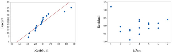
Figure 1.
The normality plots of the residuals in the 1 oz stylus tapping task using the Canon model with IDFitts. The left side is residual vs. response percentage in AD test; the right side is residual vs. IDFitts. Both plot patterns show violation of the normality assumption.
Notice that, even though the residuals met the normality requirement, this did not guarantee satisfaction of the linearity. Figure 2 presents the residual analysis in the Power model for the 1 oz data. The p-value in the AD test was 0.542, and the graph on the left shows that the scatter points fitted the straight line well. However, the graph on the right shows a parabola with a downward opening. The data violated the independent assumptions underlying the linear regression again. The lack-of-fit assumes that observations of a response variable for a given predictor variable are (1) normally distributed and (2) independent, and that (3) the distribution of the response variable has constant variance. These assumptions could be checked visually with the residuals plot. Figure 2 implied that even though the residual followed the normal distribution, it might violate the assumption of independence.
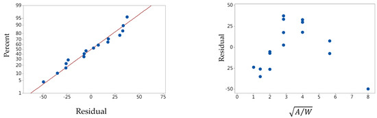
Figure 2.
The normality plots of the residuals in the 1 oz stylus tapping task using the power model. The left side is residual vs. response percentage in the AD test; the right side is residual vs. . The residuals changed the plus/minus signs as compared with Figure 1, and the plot pattern indicated violation of the assumption of independence.
Figure 3 demonstrates the advantage of the SQRT_MT model in the residuals. For the normality plot using the AD test, the scatter points are perfectly fitted along the straight line in the graph on the left. The scatter pattern of residual vs. ID also implies that the requirement of independence and the constant variance underlying the linear regression were not violated.
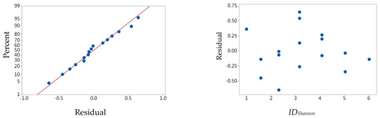
Figure 3.
The normality plots of the residuals in the 1 oz stylus tapping task using the SQRT_MT model with IDShannon. The left side is residual vs. response percentage in the AD test; the right side is residual vs. IDShannon. The normality assumption was satisfied.
This study hypothesized that MT is related to ID with the same amplitude limitation; however, this hypothesis cannot be tested with Fitts’ data, as mentioned in the literature review. Nevertheless, a trial study using Fitts’ data is possible. Table 3 presents the performances of 1 oz stylus tapping with the same amplitude considered. Compared with the pooled amplitude performances in Table 1, the much worse performance in PRESS/SSE is a distinct difference. The overall mean ratio was 5.71. The maximum ratio, 7.33, occurred at the 16-inch amplitude in the Power model. In contrast, the minimum ratio was 3.06 at the 8-inch amplitude for the SQRT_MT model with IDWelford. Although all models passed the residual normality assumption and had considerable R-squared results, the high PRESS/SSE ratio still indicated that the model was not appropriate.
Table 3.
Performances of 1 oz stylus tapping for the same amplitude with Fitts’ data [1]. The performances in all statistics but PRESS/SSE were good.
As each ID had only one observation, the lack-of-fit test could not be implemented. Generally, we use all the observations to develop a regression equation to predict these observations. The PRESS avoids this dilemma by predicting each observation based on a model developed using all other observations. The PRESS is always larger than SSE because a case deleted in fitting can never be as good as a case included. Consequently, the PRESS/SSE ratio is a supplement for evaluating whether the model fits the observations adequately in this situation.
Figure 4 presents the relationships between the MT and the ID at the same amplitude. The upward curve noted by Welford [14] existed for every amplitude, which might explain the high PRESS/SSE ratio.
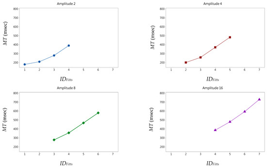
Figure 4.
Movement time vs. IDFitts in the 1 oz stylus tapping task with the same amplitude. All the plots show upward curves, which cause the PRESS to be much worse than the SSE.
On the other hand, the R-squared values were higher for the same amplitude in Table 3 than for the pooled amplitude in Table 1, but not for the 2-inch amplitude. The curvature in the 2-inch amplitude was more remarkable than the others in Figure 4, which might explain the lower R-squared results. Such a distinct curvature might have resulted from ballistic movement at the low ID [14]. The effect of ID type was the same as that for the pooled amplitude. IDShannon had the best performance, followed by IDWelford and IDFitts, for each amplitude. Overall, the R-squared performance of the SQRT_MT model was better than those of the Power and the Canon models for every amplitude.
Table 4 shows the performances of 1 lb stylus tapping with the same amplitude. Equally, IDShannon had the highest R-squared results, followed by IDWelford and IDFitts, in the Canon and SQRT_MT models for each amplitude. However, the R-squared results of the Power model were better than those of the SQRT_MT and the Canon models for all but the 16-inch amplitude. However, both the maximum and minimum PRESS/SSE ratios occurred with the 16-inch amplitude. The Power model had the worst performance, with a ratio of 6.80. In contrast, the SQRT_MT model with IDFitts performed the best, with a ratio of 2.97.
Table 4.
Performances of 1 lb stylus tapping at the same amplitude using Fitts’ data [14]. The performances in all statistics but PRESS/SSE were good.
The upward curve is a design flaw in that there is only one observation for each predictor variable. Due to this flaw, none of the models in Table 3 and Table 4 with a high PRESS/SSE ratio were appropriate for the regression analysis. The SQRT_MT model’s advantage was not shown at the same amplitude; however, the SQRT_MT model performed excellently with the pooled amplitude in Table 1 and Table 2.
If there is strong evidence that the linear regression is not appropriate, the next step in the regression analysis is to conduct a transformation. The Box–Cox procedure automatically executes the family of power transformations on the response variable. Generally, the user specifies a numerical range for the parameter lambda: the response variable’s power. When the lambda is equal to 0.5 for the Canon model, it is identical to the proposed SQRT_MT model, Equation (14), in this study. Nevertheless, the inspiration from the physiological aspect inspiration makes the SQRT_MT a causality and not just a statistical relation between MT and ID.
In summary, the SQRT_MT model demonstrates better results in the statistical requirements for the regression analysis than do the Canon and the Power models. Additionally, IDShannon achieves better performance than do IDWelford and IDFitts. With IDShannon applied, the SQRT_MT model might be the robust option for Fitts’ law application.
This study’s first purpose was to propose an alternative to the Canon model with satisfaction of the normality of residuals assumption and the statistical principle of regression analysis for researchers, and it has been achieved by succinct derivation and validation using historical data in the literature. The results in Table 1 and Table 2, as well as those in Figure 3, also demonstrated that purpose 2, applicability to ballistic movement, was also achieved.
2.3. Design of Experiment for Study Purpose 3: MT Is Related to ID with the Same Amplitude Limitation
A 24-inch/full HD resolution projected capacitive touch monitor (model: Nextech NTSP240) and an optical mouse (model: ASUS MM-5113) were applied in the experiment. The experimenter developed specific software to display the targets and record hit positions and durations. A conservative and straightforward rule proposed by Zhai et al. [50] was used to remove hitting outliers. Figure 5 illustrates the set-up of the experiment.
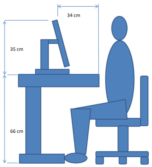
Figure 5.
The apparatus set-up in this study. The screen was located on a 66 cm high desk and angled backward; the top edge of the screen was 35 cm from the desktop in the vertical direction, and the bottom edge of the screen was 34 cm from the desk edge near the participant. Participants sat on a chair and adjusted the seat height until they felt comfortable operating the apparatus.
Twelve students (5 males and 7 females) served as the participants. They were 25.3 ± 2.6 (mean ± standard deviation) years old and 164.7 ± 7.3 cm in height. All were right-handed with no history of upper arm injury. Figure 6 shows the procedure of the experiment. In each treatment, the participants were asked to tap the targets 25 times. The timing began at the first hit and ended at the twenty-fifth hit. Twenty-four response times of twelve participants in the same treatment were averaged as the MT. Session 1 was designed as a training session to familiarize the participants with the tasks. Data acquired from sessions 2 and 3 were used for the analysis.
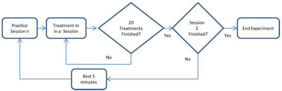
Figure 6.
The procedure of the experiment implemented in this research. Every participant began each session with a practice task, A128/ID2. There were three sessions for each participant. Twenty treatments were randomly conducted in a session. After each session finished, the participants were allowed to rest for five minutes or until they felt they had recovered from any fatigue before beginning the next session.
Instead of the traditional manipulation of target width as an independent variable to vary the ID values at the same amplitude, this research fixed ID values at 2, 3, 4, 5, and 6 (ID2, ID3, ID4, ID5, and ID6) within the amplitude. The movement amplitudes were set at 128, 256, 512, and 1024 (A128, A256, A512, and A1024) device-independent pixels. One device-independent pixel is equal to a square 0.265 mm in width. We treated the index of difficulty under a specific amplitude, ID(A), as a factor in this research. Accordingly, the target widths (W) were determined by the ID and A. Every participant completed the experiment in three sessions on the same day. There were 20 randomized treatments, 20 ID(A), in each session.
This study challenged Fitts’ argument that MT is related only to ID regardless of amplitude, based on the reported results in the literature. Instead, this research hypothesized that MT was related to ID, but the relationship should be considered under the same amplitude. Thus, the null hypotheses are:
Thirty tests () were planned to test the hypothesis of this research for the third purpose. The Dunn–Šidák procedure, one of the a priori tests suggested by Kirk (Kirk, 2013), was applied in this study. The familywise confidence level was 0.95. Consequently, the individual confidence level was 0.9983.
To explore the effects of amplitude and target width, these two variables were applied in analysis of variance (ANOVA) with a significance level of 5%. Tukey’s test with a 5% familywise level of significance was utilized for the significant factors in the ANOVA.
The experimental data were used to compare the coefficient parameters and performance indexes of the Canon, Power, and SQRT_MT models. Model performance was assessed by the normality of the residuals, the adequacy of the fitting, and the criteria for model selection.
3. Results and Discussion
3.1. Hypothesis Test on MT Is Related Only to ID
One of Fitts’ hypotheses [1] is as follows: “The average time per response will be directly proportional to the minimum average amount of information by the particular conditions of amplitude and tolerance.” This statement implies that the average movement time will be identical for the same ID even with variations in movement amplitude and target width. Fitts thought the logarithmic term of the amplitude/width ratio was the minimum average amount of information. To achieve the third purpose of this study, namely, testing the hypothesis that MT is related only to ID, as claimed by Fitts, this study designed an experiment with repetition of each ID for each amplitude. Table 5 presents the a priori test of the hypothesis mentioned in Equation (15). Generally, 26 out of 30 planned contrasts differed significantly. Consequently, MT might not be related only to ID. The possible reason might be the confounding factor, ID, as Guiard [43] indicated. The proper solution to this problem is to disaggregate ID into two individual factors, A and W.
Table 5.
Dunn-Šidák simultaneous test for the planned contrasts, indicating that most of the tasks with the same ID do not have identical MTs.
Since the ID cannot be the only dominant factor in MT, this study was examined the effects of amplitude and target width on MT. An ANOVA showed both A (F3,33 = 148.49) and W (F7,77 = 40.18) were significant, with p-values less than 0.001. Table 6 presents the post hoc test for amplitude. All the p-values of the Tukey pairwise comparisons were less than 0.001. This result implied that the MT is dependent on varied amplitude: a greater amplitude requires more MT. Likewise, Table 7 presents the results of the post hoc test for target width. Almost all p-values of the Tukey pairwise comparisons were less than 0.001, except that of 256 − 128, which was 0.002. The result implied that MT is dependent on varied target width, as well. However, MT is negatively related to target width; a smaller target width requires more MT.
Table 6.
Tukey simultaneous tests for differences of means in amplitude. The larger the amplitude was, the longer the MT was.
Table 7.
Tukey simultaneous tests for differences of means in width. The smaller the width was, the longer the MT was.
In Table 5, all six planned contrasts were significant at ID2 except (128, 256). When the difference between the paired amplitude was not huge, as in the cases of (128, 256), the contrast in MTs was just marginally not significant, since the lower bound of the simultaneous 95% confidence interval was near zero. In contrast, when the difference between the amplitudes increased, the difference in MT tended to be more significant. In the easiest task, the contribution of movement amplitude to MT was more than that of target width. For example, for target widths of 64 and 512, the amplitudes were 128 and 1024 pixels in the 2(128) − 2(1024) contrast. The absolute mean difference in MT of the 128 − 1024 contrast in the movement amplitude was 298.3 msec, and that of 64 − 512 in the target width was 128.3 msec. Similarly, this study found that the contribution of amplitude was more than that of width in all six planned contrasts at ID2. The smallest target width was 64 pixels at ID2, which was still wide enough for participants to hit the target quickly. The trade-off effect of speed vs. accuracy was not evident in the easiest task.
Results similar to those for ID2 occurred at ID3, ID4, and ID5. With increases in difficulty, the effect of width was gradually revealed. The 3(256) − 3(128), 4(256) − 4(128), and 5(256) − 5(128) contrasts were again the only non-significant contrasts at ID3, ID4, and ID5. However, two contrasts, 4(512) − 4(256) and 4(512) − 4(128), were marginally significant at ID4. Equally, 5(512) − 5(256) and 5(512) − 5(128) were marginally significant at ID5. All the adjacent amplitudes that were less than 128 pixels were not significant at ID2 to ID5. However, all six planned contrasts were significant at ID6. Only 6(512) − 6(256) and 6(256) − 6(128), but not 6(512) − 6(128), were marginally significant at ID6. Generally, the significance increased gradually as the difference in adjacent amplitudes increased. Such results imply that a reduced target width in a harder task causes participants to employ a speed–accuracy trade-off policy.
This study reanalyzed Fitts’ data (Fitts, 1954) by considering amplitude and width as factors. The ANOVA results indicated that both amplitude (F3,9 = 101.08) and width (F3,9 = 98.56) had p-values less than 0.001 in the 1 oz stylus tapping task. Equally, amplitude (F3,9 = 77.40) and width (F3,9 = 81.40) had p-values less than 0.001 in the 1 lb stylus tapping. All factors’ levels were significantly different, since they were in different groups, according to the Tukey pairwise comparison test (Table 8). Thus, MT increases as A increases or W decreases. Although the apparatus in this study differed from that in Fitts’, the effects of amplitude and target width on movement time were consistent. This raises a new question that we may have to examine carefully. Fitts’ law combines two significant factors into a single factor. Could this factor indicate that the effects of the two factors on the response time are still an unknown issue? Fortunately, we could overcome this issue by considering Fitts’ law with an underlying constant amplitude, since we would like to reject the null hypothesis. In this way, the only factor we have to investigate is the target width.
Table 8.
Tukey simultaneous tests for the effects of amplitude and target width effect on MT in 1 oz and 1 lb stylus tapping from Fitts’ data [1] had results consistent with those in this study.
In summary, this study suggests applying Fitts’ law with an underlying constant amplitude. Based on our findings: (1) target width is a significant factor in MT. This result is consistent with Hoffmann and Sheikh’s findings [51]. When the width is sufficiently narrow, people extend the MT due to the speed–accuracy trade-off. (2) The fact that amplitude significantly affects MT is consistent with Accot and Zhai [52]. (3) This paper is the first to develop a statistical inference about Fitts’ law’s implication that MT is not related only to ID. Our results support Gan and Hoffmann’s argument that amplitude affects MT and is independent of the index of difficulty [5].
3.2. Validation of the SQRT_MT Model for the Same Amplitude
The robustness of the proposed SQRT_MT model was verified with the data of this research. Since in this research, the practice effect, unlike the results in the literature [53,54], was more significant in session 1 than in sessions 2 and 3, the regression analysis was processed by excluding the data from session 1.
Table 9 presents the regression analysis using data with all the amplitudes. Although all the models fitted the linearity well and the PRESS/SSE ratios were almost perfect, around 1.11, the R-squared values, which were around 0.80, were somewhat lower than the reported value of 0.95 in the literature. IDShannon produced a higher R-squared value than IDWelford and IDFitts in both the Canon and SQRT_MT models. Additionally, the R-squared values of the SQRT_MT model were always higher than those of the Canon model for each ID type. The R-squared value of the Power model was between those of the SQRT_MT model and the Canon model. Nevertheless, none of the models satisfied the residual normality requirement.
Table 9.
Regression analysis using data for all amplitudes. The R-squared values were much lower than the value reported in the literature, possibly due to the equal observations of each ID. Additionally, the normality in all models was significant.
Figure 7 illustrates the results. The scatter points in the graph on the left, distributed straight along the regression line, satisfy the linearity adequately in the lack-of-fit test. A straight line passes through the dots’ centers at each ID, making the PRESS deviate from SSE slightly. The equal observations of each ID differed from the pattern of Fitts’ data [1], which caused the worse R-squared values. However, the variance of the fitted values increased as the ID decreased. Such a result implies a violation of the constant variance assumption in the regression analysis. The graph on the right in Figure 7 presents the regression analysis under the same amplitude. The slopes of these regression lines are different, which explains the unsatisfied residual normality.
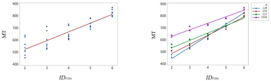
Figure 7.
The scatter plot with the regression line. The regression line in the graph on the left presents the results for IDFitts in the Canon model with all observations. It implies that the variances of varied ID were not equal. For the same amplitude for regression analysis, the graph on the right shows that the slopes of the lines are different.
It was expected that the residual normality would not be satisfied. Table 5 implies that the MTs of a specific ID with varied amplitude would be entirely different from one another at a low ID. When the difference in adjacent amplitudes at a more difficult ID is sufficiently small, the MT does not differ much. With increases in ID, the narrow width extends the MT due to participants’ speed–accuracy trade-off to compensate for the gap due to the amplitude. Such a result implies the unequal slopes of the regression lines with the varied constant amplitude. The unequal slopes also imply a possible interaction between amplitude and target width. The graph on the right in Figure 7 supports the existence of such an interaction.
This study’s hypothesis, namely, that MT is related to the ID at the same amplitude, was validated in Section 3.1. A further regression analysis considering the same amplitude was executed. Table 10 presents the parameters and test statistics required for an appreciable linear regression line considering the varied constant amplitude. Generally, the results were almost perfect, except that the Canon model applying IDFitts failed the lack-of-fit test at an amplitude of 256 pixels.
Table 10.
Regression analysis with the amplitudes separated; only one failed the test of normality (Canon IDFitts).
All the models strongly satisfied the residual normality requirement. The PRESS/SSE ratios, which ranged between 1.51 and 1.89, also performed well. For the effect of ID type on PRESS/SSE ratio, all three IDs were compatible. However, the SQRT_MT model had a minor advantage over the Canon model. The Power model provided the best and the worst ratios twice, respectively.
The R-squared values ranged from 0.964 to 0.991, and the mean was 0.978. The maximum resulted at an amplitude of 128 pixels when the SQRT_MT model with IDShannon was applied. In contrast, the minimum resulted at an amplitude of 256 pixels when the Canon model with IDFitts was applied. Among the four amplitudes, the values of IDShannon were the highest or second highest, with a difference of 0.001.
This research utilized a heuristic procedure for model selection (Table 10). The procedure was as follows: (1) both the lack-of-fit and the residual diagnostics must be satisfied. (2) Consider both the PRESS/SSE and the R-squared simultaneously, and take a trade-off policy, such as the difference between a PRESS/SSE within 0.01 and an R-squared of less than 0.1. Researchers could set the threshold values themselves. Overall, the SQRT_MT model performed slightly better in terms of R-squared than did the Power and the Canon models at the four constant amplitudes.
As mentioned in Section 2.2, the regression formulations at the same amplitude using Fitts’ data did not satisfy the linearity due to only one observation being conducted for each predictor variable’s level, which caused the scatter points to resemble a curve. The experiment in this study remedied this flaw, and the results in Table 9 imply that the last piece of the puzzle in the argument of this research, namely, that Fitts’ law should consider IDs at the same amplitude, was found.
In summary, when Fitts’ law is considered at the same amplitude, Table 3, Table 4, and Table 10 show that all models pass the residual normality test and the lack-of-fit test except the amplitude of 256 pixels with IDFitts in the Canon model. The effects of IDShannon, IDWelford, and IDFitts on R-squared consistently range from high to low, whether in the Canon or the SQRT_MT model. The same ID type always has a higher R-squared value in the SQRT_MT model than in the Canon model. Conversely, the results in Table 1, Table 2, and Table 9, for which different amplitudes were used in the formulation, show the insufficiencies in the normality assumption or the inadequacy in the data fitting. Comparison of the results between Table 1, Table 2, and Table 9 and Table 3, Table 4, and Table 10 implies that the SQRT_MT model considering the same amplitude of movement is a better choice than the Canon model using all the amplitudes simultaneously in a Fitts’ law application. Additionally, the SQRT_MT model with IDShannon performed excellently and robustly with both the data from the experiment in this study and the historical data in the literature, suggesting that it might be an excellent option for applications of Fitts’ law.
3.3. Model Selection for Application
The Canon model cannot describe the relationship between movement time and index of difficulty, possibly due to ballistic movement, as has been reported [5,22,23,24,25]. Researchers proposed the Power model to deal with this phenomenon. Furthermore, the most up-to-date theoretical literature in 2018 reported a non-linear model of the speed–accuracy trade-off [55], indicating that researchers are still looking for a consistent model for cross-comparison of results from different studies. Although proponents of the Power law emphasized that the information theory-based formulation was an invalid analogy to Shannon’s Theorem 17 and derived the power law from a human’s theoretically optimal movement, this ideal optimal behavior might be challenging to validate in the real world. Additionally, the Power model resulted in a higher R-squared value for Fitts’ data compared with the information theory-based formulation using IDFitts [8,26]. Nevertheless, the Canon model, based on information theory, remains mainstream in Fitts’ law applications. The possible reason might be the magic of information theory, which provides an attractive explanation of the information transmitted in a specific task. This characteristic facilitates the evaluation or comparison of the performances of various devices, not just the times needed to complete the same job. Oppositely, the square root of the A/W ratio is meaningless. Consequently, the Canon model is popular among researchers and industrial practitioners.
Fitts was not entirely consistent on the analogy to information theory. As Fitts himself stated, “The index of difficulty is not an exact measure of information” [56]. Additionally, the statement “the analogy with Shannon’s Theorem 17 is not exact” was printed in note 3 in Fitts and Peterson [15]. On the other hand, Fitts tried to rationalize this analogy aggressively even though he knew this analogy was problematic. Fitts defined IDFitts as the only information necessary for a movement with the amplitude and the target width specified by IDFitts [1]. IDFitts involves the amplitude and the width as metrics in length, but not in power, as Shannon’s Theorem 17 does. However, Fitts still utilized ID as the information in bits for various human movement analyses.
Since the first alternative to ID appeared in 1960 [14], the issue of which version is valid has persisted. Fitts and Peterson [15] criticized the use of IDWelford and suggested that the choice between IDFitts and IDWelford should rest on heuristic considerations, since neither of them had been derived formally from a theory. By the same token, IDShannon was not a formal derivation, either. MacKenzie also had similar thoughts, stating, “It is an engineering issue to choose a higher correlation formulation” and “the only concern was utility,” in his reply to Hoffmann’s challenge [16] on the valid version issue [42].
The Canon model describes movement time as related only to the index of difficulty, which implies that movement time is the same for the same ID value regardless of the A/W combination. After half a century, our research is the first study to test this essential hypothesis. Our results indicate that movement time is positively related to index of difficulty when the movement amplitude is the same for different ID values. Consequently, Fitts’ law should be applied to each movement amplitude individually. In this way, the failure in the normality of residuals and the lack of adequate fitting, which have long been ignored and unreported in the literature, can be avoided.
This research focused on the facts about Fitts’ law in the literature that we have mentioned but were ignored by researchers. Fitts [15] clearly stated that the analogy to Shannon’s Theorem 17 is not proper [56], the ID is not formally derived from information theory [11,15,17,26,42], and the selection between candidates relies on researchers’ heuristic considerations. Despite the fact that the analogy of the Canon model to information theory is still controversial in research [16,39,40], the mathematical proofs in these studies suffer the same validation challenge in natural human movement as in the Power model. Human movements might approximate the theoretical argument, but minor deviations could impact the fitness of the formula. Nevertheless, the experimental data in the literature published over the past sixty-five years demonstrate that the positive relationship between movement time and index of difficulty holds true. This research proposes a modified model, the SQRT_MT model, to improve the formula in terms of satisfying the underlying statistical assumption. Furthermore, the SQRT_MT model combines findings from the fields of psychology, physics, and physiology. It is a model that considers theoretical advances in modern physics and physiology, and empirical results from psychology and physiology can be considered simultaneously. This research has demonstrated that the SQRT_MT model has advantages both in the statistical requirements and the realistic fitness of ballistic movements. Hopefully, the SQRT_MT model will shed the light on the unification of Fitts’ law in one formula.
The above results imply that it is more suitable to treat all the Fitts’ law models simply as prediction models for response time. Based on the results of this research listed in Table 10, all the available options in Fitts’ law have excellent performance in a proper experimental design. This research agrees with Fitts [17] and MacKenzie’s argument [42]; researchers can choose their preferred model heuristically. Therefore, the issue of which version is valid should not persist in the community.
To summarize, the approach to modeling the prediction of movement time by applying the same amplitude with repetition for each predictor variable and proper diagnostics for the linear regression’s assumptions should be considered in Fitts’ law. Researchers can select any prediction formulation they prefer: the Canon, the Power, or the SQRT_MT model. The SQRT_MT model with IDShannon is suggested based on the high R-squared value, the satisfied normality of residuals, and the adequate fitting with empirical data in the historical and current experiments.
3.4. Meaning of the Intercept and the Slope
Some researchers have claimed that the non-zero intercept was caused by a modeling error [24,57] or resulted from not using IDShannon [18,21]. Those authors might think that movement time should be zero when ID is zero. However, ID is never zero in the real world [15]. Fitts designed the ID to be more than zero [1]. No matter how easy a movement is, it entails slight difficulty. Zero difficulty would imply a total lack of movement. That might be the reason why Fitts added the constant multiplier, 2, in the definition of ID.
Other reasons, such as the time required for movement of zero distance [21], the dwell time on the target in reciprocal tapping [17], and submovements such as the pressing time of a mouse button [21], do not explain the zero intercept, either. Movement time is always measured from the moment of departure from the starting point to the moment of contact with the target. The time required for motor unit recruitment before the movement occurs, i.e., the time for zero distance, might be impossible to record with the apparatus in the reported literature.
Theoretically, whether the intercept equals zero or not should be determined by a t-test based on empirical data. Many possible meanings of the intercept have been reviewed in the literature [4,50]. Fitts designed the ID never to be zero by multiplying by 2 in the logarithmic term. Additionally, neither IDWelford nor IDShannon is zero, theoretically. Since the intercept is a derived value from the regression analysis and there is no theoretical reason for it to be zero, its calculation and explanation must obey the statistical principle. Kunter et al. [44] indicated that the intercept does not have any particular meaning if a horizontal axis variable equal to zero does not exist. Fitts’ law satisfies this kind of case. All of the arguments about the zero intercept might be unnecessary.
The most attractive index, slope “b” in Equation (2), was proposed to underlie the analogy to Shannon’s Theorem 17. However, this explanation would not work if the intercept, “a” in Equation (2), were not zero. Unfortunately, “a” is seldom zero in the empirical data.
Moreover, we have argued that all the Fitts’ law models should be treated as simple prediction equations for response time with the supporting evidence in the literature in Section 3.3. In normal circumstances, ID is not required information, nor is the information transmission rate.
In short, the intercept is meaningless because the predictor variable, ID, is never zero in the real world. Similarly, the slope is the rate of change in movement time for the unit change in ID.
4. Conclusions
To conclude, the present study presents primary research on Fitts’ paradigm. Still, it reveals some essential requirements and assumptions of the linear regression analysis that were not satisfied in past research. The major contributions of this research are as follows: (1) this is the first study to conduct a formal hypothesis test for the essential assumption, namely, that MT is related only to ID, in the literature. The results indicate that MT is related to ID at the same amplitude. Researchers might apply Fitts’ law for varied amplitudes. (2) The SQRT_MT model provides excellent results in all the required statistics of linear regression. The proposed SQRT_MT model, combining findings from the fields of psychology, physics, and physiology, in combination with IDShannon, might be a robust option for Fitts’ law application. In addition, it is a simple and easy-to-apply model that tolerates both ballistic and visual feedback movement concurrently. (3) The approach to modeling the prediction of movement time should utilize repetition in each predictor variable, and proper diagnostics for the linear regression’s assumptions should be considered. (4) The results of the experiment in this research show that all the available models are excellent prediction equations. Researchers can choose their preferred model for their investigations. (5) The proposed SQRT_MT model might shed light on the unification of Fitts’ law in one formula.
Although this study’s three purposes were achieved, some limitations must be noted. (1) The SQRT_MT model was demonstrated to tolerate both ballistic and visual feedback movement concurrently with the historical data in the literature, but it is believed that no ballistic movement was present in this study, since the shortest MT in this study was much longer than 200 msec. (2) The linearity fitting and the residual assumption were strongly satisfied by the results of the experiment, too. However, the repetition in each predictor level at the same amplitude is two. Future research is suggested to improve the two limitations to enhance the validity of the SQRT_MT model.
Author Contributions
Conceptualization, C.J.L. and C.-F.C.; methodology, C.-F.C.; software, C.-F.C.; validation, C.J.L. and C.-F.C.; formal analysis, C.-F.C.; investigation, C.J.L. and C.-F.C.; resources, C.J.L.; data curation, C.-F.C.; writing—original draft preparation, C.-F.C.; writing—review and editing, C.J.L.; visualization, C.-F.C.; supervision, C.J.L.; project administration, C.J.L. Both authors have read and agreed to the published version of the manuscript.
Funding
This research received no external funding.
Institutional Review Board Statement
The study was conducted according to the Declaration of Helsinki guidelines and approved by the Ethics Committee of National Taiwan University (protocol code NTU-REC No.: 201302HS009 and approval date: 27 May 2020).
Informed Consent Statement
Informed consent was obtained from all subjects involved in the study.
Acknowledgments
The authors would like to thank Yi-Chun Lin and Ching-Yu Lin for their assistance in recruiting the participants, conducting the experiment, and collecting raw data.
Conflicts of Interest
The authors declare no conflict of interest.
References
- Fitts, P.M. The information capacity of the human motor system in controlling the amplitude of movement. J. Exp. Psychol. 1954, 47, 381. [Google Scholar] [CrossRef] [PubMed]
- Hoffmann, E.R.; Drury, C.G.; Romanowski, C.J. Performance in one-, two-and three-dimensional terminal aiming tasks. Ergonomics 2011, 54, 1175–1185. [Google Scholar] [CrossRef]
- Plamondon, R.; Alimi, A.M. Speed/accuracy trade-offs in target-directed movements. Behav. Brain Sci. 1997, 20, 279–303. [Google Scholar] [CrossRef]
- Soukoreff, R.W.; MacKenzie, I.S. Towards a standard for pointing device evaluation, perspectives on 27 years of fitts’ law research in hci. Int. J. Hum. Comput. Stud. 2004, 61, 751–789. [Google Scholar] [CrossRef]
- Gan, K.-C.; Hoffmann, E.R. Geometrical conditions for ballistic and visually controlled movements. Ergonomics 1988, 31, 829–839. [Google Scholar] [CrossRef]
- Hoffmann, E.R.; Sheikh, I.H. Finger width corrections in Fitts’ law: Implications for speed-accuracy research. J. Mot. Behav. 1991, 23, 259–262. [Google Scholar] [CrossRef]
- Hoffmann, E.R. Fitts’ law with transmission delay. Ergonomics 1992, 35, 37–48. [Google Scholar] [CrossRef]
- Meyer, D.E.; Abrams, R.A.; Kornblum, S.; Wright, C.E.; Keith Smith, J. Optimality in human motor performance: Ideal control of rapid aimed movements. Psychol. Rev. 1988, 95, 340. [Google Scholar] [CrossRef] [PubMed]
- Goldberg, K.; Faridani, S.; Alterovitz, R. Two large open-access datasets for fitts’ law of human motion and a succinct derivation of the square-root variant. IEEE Trans. Hum. Mach. Syst. 2015, 45, 62–73. [Google Scholar] [CrossRef]
- Jagacinski, R.J.; Repperger, D.W.; Ward, S.L.; Moran, M.S. A test of fitts’ law with moving targets. Hum. Factors 1980, 22, 225–233. [Google Scholar] [CrossRef]
- Kvålseth, T.O. An alternative to fitts’ law. Bull. Psychon. Soc. 1980, 16, 371–373. [Google Scholar] [CrossRef]
- Grosjean, M.; Shiffrar, M.; Knoblich, G. Fitts’s law holds for action perception. Psychol. Sci. 2007, 18, 95–99. [Google Scholar] [CrossRef] [PubMed]
- Shannon, C.E. A mathematical theory of communication. Bell Syst. Tech. J. 1948, 27, 379–423. [Google Scholar] [CrossRef]
- Welford, A.T. The measurement of sensory-motor performance: Survey and reappraisal of twelve years’ progress. Ergonomics 1960, 3, 189–230. [Google Scholar] [CrossRef]
- Fitts, P.M.; Peterson, J.R. Information capacity of discrete motor responses. J. Exp. Psychol. 1964, 67, 103. [Google Scholar] [CrossRef]
- Hoffmann, E.R. Which version/variation of fitts’ law? A critique of information-theory models. J. Mot. Behav. 2013, 45, 205–215. [Google Scholar] [CrossRef] [PubMed]
- Fitts, P.M.; Radford, B.K. Information capacity of discrete motor responses under different cognitive sets. J. Exp. Psychol. 1966, 71, 475. [Google Scholar] [CrossRef]
- MacKenzie, I.S. A note on the information-theoretic basis for fitts’ law. J. Mot. Behav. 1989, 21, 323–330. [Google Scholar] [CrossRef]
- MacKenzie, I.S.; Sellen, A.; Buxton, W.A. A comparison of input devices in element pointing and dragging tasks. In Proceedings of the SIGCHI Conference on Human Factors in Computing Systems, New Orleans, LA, USA, 27 April–2 May 1991; pp. 161–166. [Google Scholar]
- MacKenzie, I.S.; Buxton, W. Extending fitts’ law to two-dimensional tasks. In Proceedings of the SIGCHI Conference on Human Factors in Computing Systems, Monterey, CA, USA, 3–7 May 1992; pp. 219–226. [Google Scholar]
- MacKenzie, I.S. Fitts’ law as a research and design tool in human-computer interaction. Hum. Comput. Interact. 1992, 7, 91–139. [Google Scholar] [CrossRef]
- Schmidt, R.A.; Zelaznik, H.N.; Frank, J.S. Sources of inaccuracy in rapid movement. In Information Processing in Motor Control and Learning; Elsevier: Amsterdam, The Netherlands, 1978; pp. 183–203. [Google Scholar]
- Schmidt, R.A. Control processes in motor skills. Exerc. Sport Sci. Rev. 1976, 4, 229–262. [Google Scholar] [CrossRef] [PubMed]
- Schmidt, R.A.; Zelaznik, H.; Hawkins, B.; Frank, J.S.; Quinn, J.T., Jr. Motor-output variability: A theory for the accuracy of rapid motor acts. Psychol. Rev. 1979, 86, 415. [Google Scholar] [CrossRef]
- Welford, A.T.; Norris, A.; Shock, N. Speed and accuracy of movement and their changes with age. Acta Psychol. 1969, 30, 3–15. [Google Scholar] [CrossRef]
- Kvåiseth, T.O. Note on information capacity of discrete motor responses. Percept. Mot. Ski. 1979, 49, 291–296. [Google Scholar] [CrossRef]
- Whisenand, T.G.; Emurian, H.H. Effects of angle of approach on cursor movement with a mouse: Consideration of Fitt’s law. Comput. Hum. Behav. 1996, 12, 481–495. [Google Scholar] [CrossRef]
- Whisenand, T.G.; Emurian, H.H. Analysis of cursor movements with a mouse. Comput. Hum. Behav. 1999, 15, 85–103. [Google Scholar] [CrossRef]
- Murata, A.; Fukunaga, D. Extended fitts’ model of pointing time in eye-gaze input system-incorporating effects of target shape and movement direction into modeling. Appl. Ergon. 2018, 68, 54–60. [Google Scholar] [CrossRef]
- Murata, A.; Iwase, H. Extending Fitts’ law to a three-dimensional pointing task. Hum. Mov. Sci. 2001, 20, 791–805. [Google Scholar] [CrossRef]
- Cha, Y.; Myung, R. Extended Fitts’ law for 3d pointing tasks using 3d target arrangements. Int. J. Ind. Ergon. 2013, 43, 350–355. [Google Scholar] [CrossRef]
- DeLong, S.; MacKenzie, I.S. Evaluating devices for object rotation in 3d. In Proceedings of the International Conference on Universal Access in Human-Computer Interaction, Las Vegas, NV, USA, 15–20 July 2018; pp. 160–177. [Google Scholar]
- Bi, X.; Li, Y.; Zhai, S. Ffitts law: Modeling finger touch with fitts’ law. In Proceedings of the SIGCHI Conference on Human Factors in Computing Systems, Paris, France, 27 April–2 May 2013; pp. 1363–1372. [Google Scholar]
- El Lahib, M.; Tekli, J.; Issa, Y.B. Evaluating fitts’ law on vibrating touch-screen to improve visual data accessibility for blind users. Int. J. Hum. Comput. Stud. 2018, 112, 16–27. [Google Scholar] [CrossRef]
- Lin, C.J.; Ho, S.-H. Prediction of the use of mobile device interfaces in the progressive aging process with the model of fitts’ law. J. Biomed. Inform. 2020, 107, 103457. [Google Scholar] [CrossRef]
- Lin, C.J.; Cheng, C.-F.; Chen, H.-J.; Wu, K.-Y. Training performance of laparoscopic surgery in two-and three-dimensional displays. Surg. Innov. 2017, 24, 162–170. [Google Scholar] [CrossRef]
- Roig-Maimó, M.F.; MacKenzie, I.S.; Manresa-Yee, C.; Varona, J. Head-tracking interfaces on mobile devices: Evaluation using fitts’ law and a new multi-directional corner task for small displays. Int. J. Hum. Comput. Stud. 2018, 112, 1–15. [Google Scholar] [CrossRef]
- Bachynskyi, M.; Palmas, G.; Oulasvirta, A.; Weinkauf, T. Informing the design of novel input methods with muscle coactivation clustering. ACM Trans. Comput. Hum. Interact. 2015, 21, 1–25. [Google Scholar] [CrossRef]
- Gori, J.; Rioul, O.; Guiard, Y. Speed-accuracy tradeoff: A formal information-theoretic transmission scheme (fitts). ACM Trans. Comput. Hum. Interact. 2018, 25, 1–33. [Google Scholar] [CrossRef]
- Müller, J.; Oulasvirta, A.; Murray-Smith, R. Control theoretic models of pointing. ACM Trans. Comput. Hum. Interact. 2017, 24, 1–36. [Google Scholar] [CrossRef]
- Drewes, H. Only one fitts’ law formula please. In Proceedings of the CHI’10 Extended Abstracts on Human Factors in Computing Systems, Atlanta, GA, USA, 10–15 April 2010; pp. 2813–2822. [Google Scholar]
- MacKenzie, I.S. A note on the validity of the shannon formulation for fitts’ index of difficulty. Open J. Appl. Sci. 2013, 3, 360. [Google Scholar] [CrossRef]
- Guiard, Y. The problem of consistency in the design of fitts’ law experiments: Consider either target distance and width or movement form and scale. In Proceedings of the SIGCHI Conference on Human Factors in Computing Systems, Boston, MA, USA, 4–9 April 2009; pp. 1809–1818. [Google Scholar]
- Kutner, M.H.; Nachtsheim, C.J.; Neter, J.; Li, W. Applied Linear Statistical Models; McGraw-Hill Irwin: Boston, MA, USA, 2005; Volume 5. [Google Scholar]
- Milton, J.S.; Arnold, J.C. Introduction to Probability and Statistics, 4nd ed.; McGraw-Hill: New York, NY, USA, 2003. [Google Scholar]
- Harris, C.M.; Wolpert, D.M. Signal-dependent noise determines motor planning. Nature 1998, 394, 780. [Google Scholar] [CrossRef] [PubMed]
- Hamilton, A.F.d.C.; Wolpert, D.M. Controlling the statistics of action: Obstacle avoidance. J. Neurophysiol. 2002, 87, 2434–2440. [Google Scholar] [CrossRef] [PubMed]
- Jones, K.E.; Hamilton, A.F.d.C.; Wolpert, D.M. Sources of signal-dependent noise during isometric force production. J. Neurophysiol. 2002, 88, 1533–1544. [Google Scholar] [CrossRef]
- Hamilton, A.F.d.C.; Jones, K.E.; Wolpert, D.M. The scaling of motor noise with muscle strength and motor unit number in humans. Exp. Brain Res. 2004, 157, 417–430. [Google Scholar] [CrossRef]
- Zhai, S. Characterizing computer input with fitts’ law parameters—the information and non-information aspects of pointing. Int. J. Hum. Comput. Stud. 2004, 61, 791–809. [Google Scholar] [CrossRef]
- Hoffmann, E.R.; Sheikh, I.H. Effect of varying target height in a fitts’ movement task. Ergonomics 1994, 37, 1071–1088. [Google Scholar] [CrossRef]
- Accot, J.; Zhai, S. Refining Fitts’ law models for bivariate pointing. In Proceedings of the SIGCHI Conference on Human Factors in Computing Systems, Fort Lauderdale, FL, USA, 5–10 April 2003; pp. 193–200. [Google Scholar]
- Zhai, S.; Kong, J.; Ren, X. Speed–accuracy tradeoff in fitts’ law tasks—On the equivalency of actual and nominal pointing precision. Int. J. Hum. Comput. Stud. 2004, 61, 823–856. [Google Scholar] [CrossRef]
- Wright, C.E.; Lee, F. Issues related to hci application of fitts’s law. Hum. Comput. Interact. 2013, 28, 548–578. [Google Scholar] [CrossRef]
- Guiard, Y.; Rioul, O. A mathematical description of the speed/accuracy trade-off of aimed movement. In Proceedings of the 2015 British HCI Conference, Lincoln, UK, 13–17 July 2015; pp. 91–100. [Google Scholar]
- Fitts, P. The influence of response coding on performance in motor tasks. In Current Trends in Information Theory; University of Pittsburgh Press: Pittsburgh, PA, USA, 1953; pp. 47–75. [Google Scholar]
- Crossman, E.; Goodeve, P. Feedback control of hand-movement and fitts’ law. Q. J. Exp. Psychol. Sect. A 1983, 35, 251–278. [Google Scholar] [CrossRef] [PubMed]


Publisher’s Note: MDPI stays neutral with regard to jurisdictional claims in published maps and institutional affiliations. |
© 2021 by the authors. Licensee MDPI, Basel, Switzerland. This article is an open access article distributed under the terms and conditions of the Creative Commons Attribution (CC BY) license (https://creativecommons.org/licenses/by/4.0/).