
On-Off Intermittency in a Three-Species Food Chain


1
Institute of Geosciences and Earth Resources, National Research Council, 10125 Turin, Italy
2
Institute of Geosciences and Earth Resources, National Research Council, 56124 Pisa, Italy
*
Author to whom correspondence should be addressed.
Mathematics 2021, 9(14), 1641; https://doi.org/10.3390/math9141641
Submission received: 24 May 2021
/
Revised: 5 July 2021
/
Accepted: 7 July 2021
/
Published: 12 July 2021
(This article belongs to the Special Issue Differential Equation Models in Applied Mathematics: Theoretical and Numerical Challenges)
Abstract
:The environment affects population dynamics through multiple drivers. Here we explore a simplified version of such influence in a three-species food chain, making use of the Hastings–Powell model. This represents an idealized resource–consumer–predator chain, or equivalently, a vegetation–host–parasitoid system. By stochastically perturbing the value of some parameters in this dynamical system, we observe dramatic modifications in the system behavior. In particular, we show the emergence of on–off intermittency, i.e., an irregular alternation between stable phases and sudden bursts in population size, which hints towards a possible conceptual description of population outbursts grounded into an environment-driven mechanism.
1. Introduction
When Batchelor and Townsend [1] observed a peculiar irregularity in a turbulent fluid, namely the alternation between sudden bursts of motion and a milder, non-turbulent activity, they used the word intermittency to describe it. Since then, the same term has been used to describe several types of switching behavior between different dynamical regimes. Here, we are especially interested in the phenomenon called on–off intermittency [2].
On-off intermittency has been observed in real systems, such as electronic circuits [3], earthquakes [4], solar cycles [5], electrodynamics of liquid crystals [6], as well as theoretically studied through numerical approaches [2,7] with specific focus on discrete-time population dynamics models (i.e., maps) [8,9,10].
The goal of this work is to expand these studies to the case of a stochastically driven system of coupled ordinary differential equations (ODEs). To this end, we include the random variability of suitable model parameters to simulate environmental stochasticity in a system representing the population dynamics of three different species. In the autonomous case, a three-dimensional ODE system is the minimum requirement to allow chaotic dynamics owing to the Poincaré–Bendixson theorem [11].
Our choice here is the well-known Hastings–Powell model [12,13], a system that describes the evolution of three species, anonymously called x, y, z, which represent primary producers (resource), consumers (or host) and predators (or parasitoids). We stochastically perturb some of the system parameters, which measure species interactions or carrying capacity, showing that on–off intermittent behaviour can emerge. This feature could qualitatively explain the onset of outbreaks (also called irruptions) in the population size of some of the ecosystem components [14,15].
Section 2 describes the properties of on–off intermittency, summarizing results from previous studies that inspired this work. Section 3 introduces the Hastings–Powell model, describes its parameters and explains the numerical approach that is adopted. In Section 4, we illustrate the occurrence of on–off intermittency when one introduces environmentally driven—and stochastically simulated—parameters. Finally, Section 5 summarizes our results and outlines some possible future developments.
2. On-Off Intermittency
On-off intermittency is characterized by the alternation between regular phases, which duration can span a rather wide range of orders of magnitude, and burst phases, where a sudden instability throws the system into (possibly) chaotic behavior. This kind of intermittency can appear in a dynamical system that has an invariant manifold (in the simplest case, a fixed point) whose stability properties depend on an external control parameter but whose phase-space position is only weakly dependent upon the same parameter.
When such control parameter has an irregular temporal variation, either stochastic or chaotic, the manifold alternates between stable and unstable conditions. In order to realize on–off intermittency, a system must keep its dynamics in the proximity of the manifold, which in the stable phases must be attractive enough to allow for long periods during which the system resides in the vicinity of the manifold. Lingering near this temporarily stable manifold, the system undergoes protracted regular phases, when suddenly the volatility of the control parameter induces the instability of the manifold and causes the system to burst away from it, leading to values which are quite different from its typical statistics.
In past years, on–off intermittency has raised some interest in the scientific community. After its basics were scouted by the work of Platt et al. [2], Heagy et al. [7] gave a mathematical sounding demonstration of the power law underlying the duration of laminar phases for maps with the specific form (with the variable coming from a random or a chaotic process), then Toniolo et al. [8] further deepened this latter aspect, inspecting the occurrence of on–off intermittency in a stochastically driven logistic map. Due to the possibility of adopting this concept to qualitatively explain ecological outbreaks, in 2010 Metta et al. [9] and Moon [10] investigated Toniolo’s framework in the context of coupled logistic equations. While the former focused on kurtosis as an index to identify on–off intermittency, the latter put the spotlight on the stability of the coupled system, employing the largest Lyapunov Exponent to quantify the chaotic dynamics occurring with different coupling strengths of adjacent logistic systems. Here, we continue the exploration of on–off intermittency in the context of ecosystem dynamics and study its presence and characteristics in a system of coupled ordinary differential equations representing a three-layer food chain.
3. Hastings–Powell Model
Alan Hastings and Thomas Powell introduced a three-dimensional dynamical system [12] in order to illustrate chaotic behavior in a food web involving three trophic levels. They employed the type 2 functional response (i.e., a Michaelis–Menten functional form) shown in the 1975 Murdoch and Oaten’s paper [16] to couple the different trophic levels of the system. The basic equations of the Hastings–Powell model are:
where X, Y, Z represent the biomass of three species on three different trophic levels and T is time. Throughout the three equations, subscripts 0, 1, 2 indicate parameters referring to, respectively, X, Y, Z. and are, respectively, the growth rate and the carrying capacity of the species X. The constants , , , characterize the functional responses among the species, representing the saturation of the response; specifically, the Bs are the prey populations that correspond to half the maximum value of the predation rate per unit prey. , are the conversion rates from resource to consumer and from prey to predator, respectively, while, finally, , are constant death rates.
A suitable nondimensionalization leads to redefine the variables of the system:
Consequently, the nondimensional parameters are:
Thus, the final equations of Hastings–Powell model are:
Hastings and Powell chose the model parameters to be, in their words, “biologically reasonable”. For example, the parameter values associated with the consumer (y) are larger than those for the predator/parasitoid (z), so that x and y interact on a faster time scale with respect to y and z. We defer to the original work of Hastings and Powell for further discussions on parameter values.
Note that Equation (8) is conceptually different from Equations (6) and (7): indeed, it is possible to factorize z on the right hand side, leading to . A separation of variables allows to retrieve the exact solution , which could replace the differential equation in the numerical simulation. This peculiarity makes Equation (8) quite different from the other two equations and, therefore, we expect it to react differently to stochastic forcing.
In Appendix A we provide a concise analysis of the fixed points in the Hastings–Powell model.
Stochastic Parameters and Numerical Simulations
To simulate how the environment affects the evolution of the three-species food chain in the Hasting-Powell model, we allow some of the model parameters to become random numbers. In particular, we allow either or in Equations (5)–(8) to vary stochastically with a uniform distribution between 0 and . The computation of the stochastic term is performed at every time step of the numerical simulation, feeding the same term throughout all the steps needed by the Runge–Kutta 4 scheme employed. The random number at each time step is independent of the previous value, that is we force the system with white noise.
The different cases are run for time units, after a spin-up time of time units to eliminate the initial transient. Initial conditions for , are randomly and uniformly chosen between 0 and 1 while the initial value for is randomly and uniformly chosen between 4 and 5. This choice for is related to the convenience of starting as close as possible to the system attractor, thus reducing the spin-up time. Laminar phases are defined as or —i.e., a distance of from the stable fixed point.
4. Results
4.1. Intensity of Grazing
The parameter measures the intensity of grazing by the consumer (y) on the resource (x) in the coupling term between the equations for x and y in Equations (6) and (7). As a first test, we replace with the random number , uniformly distributed between 0 and . In this way, the time-averaged value of becomes . Therefore, the coupling between x and y becomes:
Here we use , which gives . For the other parameters we adopt the same values as in the original paper of Hastings and Powell, namely:
Figure 1 shows the time series of the three trophic levels (x, y and z) and a running mean of the instantaneous value of . The time series of the resource x and of the herbivorous y visually illustrate the occurrence of on–off intermittency, with the alternation of long laminar phases and irregularly spaced bursts. The laminar phases of x are centered on , corresponding to a fixed point of the system, and the bursts are towards lower values when the herbivorous density suddenly increases. The z signal, instead, corresponds to a smoothed version of the intermittent signals and it is slightly delayed with respect to the herbivorous dynamics, as expected from the form of the equations.
As mentioned above, the simplest case of on–off intermittency appears when the stability of a fixed point of the system depends on an external parameter that varies irregularly in time, thus determining an alternation between stability and instability of the fixed point. To motivate our choice of , in Figure 2 we show the orbit diagram for y in the range (the orbit diagram for x is conceptually similar). In order to find on–off intermittency, we need to span a parameter range covering the interval between stability and chaos. The chosen value of suits this well, forcing the instantaneous value of to vary between 0 and 3.5. From Figure 1, one sees an approximate correspondence between intermittent bursts and periods when the running average of exceeds its average value which, in this case, approximately corresponds to the stability limit of the fixed point.
The first distinctive feature of on–off intermittent time series is the shape of the probability distribution of the off-phase durations—i.e., the number of time steps in which the system endures off (laminar) behaviour. It has been shown that for a simplified type of discrete maps [7,8], for on–off intermittency the distribution of laminar phase duration, D, follows a power law, . Figure 3 shows that, also for this continuous on–off intermittent system, the x and y signals display the same approximate power-law distribution of off phases, at least in a limited range of off-phase durations.
Another characteristics of the intermittent signals is the broad distribution of the amplitudes. Figure 4 shows the distribution of maxima for on–off intermittency and for standard chaotic behavior with a fixed value . An approximate power-law distribution of the maxima is evident for the intermittent dynamics.
Conceptually, inserting the stochastic term as done in Equation (9) is tantamount to randomly forcing in Equations (1) and (2). Thus, the results presented in this section indicate that the environmental fluctuations (represented by the stochastic term), randomly influencing the rate of successful consumption by y of the resource x, can cause on–off intermittency in both compartments.
4.2. Carrying Capacity
Another interesting option is to allow the environment to stochastically affect the system carrying capacity, . Even though and are mathematically related, their ecological meaning is different: the former is related to the interaction between x and y and the latter only to the maximum value of x in the absence of consumers. Therefore, they deserve separate analyses from an ecological standpoint. Looking at Equation (5), we infer that to this end we must multiply , , and in Equations (6)–(8) by the same value of a random number , uniformly distributed in the interval . The parameters chosen for this Section are the same described in Equation (10), with . Following the rationale that yielded Equation (9), the couplings in Equations (6)–(8) become:
Choosing different values for leads to different and peculiar behaviours.
From to the system undergoes a long lasting stability at , , . For we observe the occurrence of on–off intermittency for x and y, while after the transient the z species becomes extinct, that is, the predator (parasitoid) cannot control the consumer (host).
Figure 5 shows the time series of x and y, along with the probability distributions of the maxima and the moving average of the value of the random number controlling . As in the case of stochastic variability in , the intermittency of the time series is matched by the fluctuations of the running mean of , with low values of the latter corresponding to laminar phases of the time series.
Figure 6 shows the probability distribution of the laminar phase durations, which matches a power law with .
For , x and y show chaotic dynamics, but the most intriguing phenomenon is related to the apparent on–off intermittency of z, as shown in Figure 7. A close inspection of the laminar phase durations, however shows that extended laminar periods are quite likely to occur, thus the curve is less steep than .
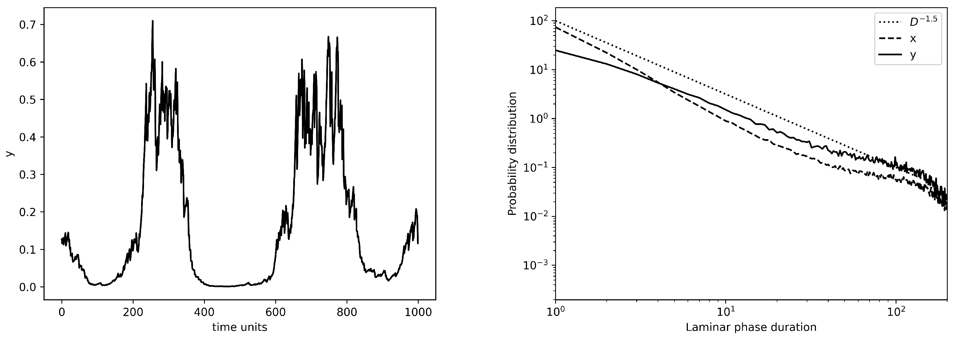
Finally, we report that at larger values of —here we employ —non-intermittent, chaotic dynamics for z is paired with approximately on–off intermittent behavior for x and y. Figure 8 shows a time series of y along with the laminar phase durations, which approximately follows the simple power law (even though less robustly than in Figure 6).
The implications of these results are intriguing. If the environment induces a random variability of the carrying capacity , allowing it to temporarily reach large enough values, on–off intermittency can emerge quite easily in both x and y—that is, in the primary producers and their consumers. By further increasing , that is, the amplitude of the random variability of , a peculiar intermittency in the predator (parasitoid) z develops. This implies that sudden bursts in a population could be induced far from the trophic level that is directly affected by the environmental fluctuations. For even larger values of the fluctuations in (), the resource and the consumer again undergo approximate on–off behavior, while the predator behaves chaotically. Clearly, the complexity of the system behavior is huge, and a deeper exploration of the different dynamics and of their ecological implications is deferred to future works.
5. Discussion and Conclusions
This paper conceptually extends the works of Platt et al. [2], Heagy et al. [7], Toniolo et al. [8] and Metta et al. [9] and it focuses on the emergence of on–off intermittency in idealized food chains. In our view, such dynamical behavior can be taken as a conceptual description of species outbreak events in different levels of the food chain.
To explore this issue, we used the Hastings–Powell model, a well-known system that allowed us to inspect a simple three-species food chain: resource, consumer and predator (or else, vegetation, pest host species and parasitoid). Environmental forcing was supposed to act on the resource dynamics, and it was represented as an imposed random variation in some of the controlling parameters.
When the stochastic variability is inserted into the parameter controlling the intensity of resource consumption (i.e., y on x, Section 4.1), on–off intermittency easily arises in both these variables, while the predator z displays a smoother dynamics.
Stochastic variability of the carrying capacity (Section 4.2) leads to intriguing results; indeed, increasing the range of random variations to higher values sequentially generates different behaviours:
- For low maximum values of the carrying capacity, we observe only a stable fixed point for and z;
- Above a threshold of the maximum value of the carrying capacity, we observe on–off intermittency in x and y, while z goes extinct;
- For larger ranges of random variations, chaotic dynamics for x and y and intermittent behavior in z;
- For still larger fluctuations, we observe weak on–off intermittency in x and y and chaotic behavior of z.
Ecologically, this suggests that a low carrying capacity for x implies that the species directly feeding on it (y) can endure but on average it does not supply enough biomass for z to survive. A slightly larger value of allows for z to “jump start”, while a higher average value of the carrying capacity is enough to fully support the predator species, bringing back on–off intermittency in the dynamics of x and y. Of course, this is just an euristic representation that requires further exploration.
Several points remain open to investigation, such as:
- Would a deterministic, chaotic system representing the environment dynamics, in place of the stochastic process adopted here, allow for a more thoroughly mathematical analysis of the problem?
- How would spatial extension, with coupling across different location of the same species, affect our results?
- How would on–off intermittency manifest itself (if it does) in a food web rather than a simple food chain?
- Can we find intermittency when using real-world datasets or controlled laboratory experiments in microcosms?
Such questions are, in our opinion, relevant to better understand bursting phenomena in ecology and will be a subject of future research, after the first demonstration of the possibility of on–off intermittent behavior in model food chains that was illustrated here.
Author Contributions
Conceptualization, G.V. and A.P.; methodology, software and validation, G.V.; writing—original draft preparation, G.V.; writing—review and editing, G.V. and A.P.; funding acquisition, A.P. All authors have read and agreed to the published version of the manuscript.
Funding
This research was partially funded by the EU H2020 project “EOTIST”, Grant Agreement no. 952111.
Institutional Review Board Statement
Not applicable.
Informed Consent Statement
Not applicable.
Data Availability Statement
Code used in numerical simulation can be found at https://figshare.com/articles/software/VissioProvenzale2021/14639556 (accessed on 8 July 2021).
Acknowledgments
The authors acknowledge the three reviewers for their insightful comments. In particular, the authors are grateful to Reviewer 1, whose observations led to the material included in Appendix A.
Conflicts of Interest
The authors declare no conflict of interest.
Appendix A. Fixed Points in Hastings–Powell Model
A thorough analysis of the fixed points of the models is beyond the scope of this paper. Nevertheless, it is useful to briefly recap them, in order to give some perspective on the results obtained, especially on the population values typically attained during the laminar phases. Checking the fixed points in the system leads to four different results:
- Computing the Jacobian and substituting these values leads to the eigenvalues 1, , . Note that the ecologically-relevant case has , so this fixed point is a saddle. If we numerically perturb the system along the x direction (e.g., adding a small perturbation to ), the system falls into the fixed point (see below) while, perturbing it along other directions, the null state is attractive.
- The three eigenvalues are , , . and are always negative, but the second eigenvalue depends on the values of the parameters . With the values used in the paper, the eigenvalue is positive and the system is therefore repulsive along one direction (it can be numerically checked perturbing ). If , then the fixed point becomes stable.
- From Equation (8), we obtain ; inserting it in Equation (6) leads to two (rather cumbersome) different solutions for and, consequently, two solutions for from Equation (7). With the parameter values adopted in this work, one solution for is negative and therefore not acceptable. The other solution is positive and, for the first case in Section 4.1 (with , as in Hastings–Powell’s paper), the fixed point is , , (numerically verified).
References
- Batchelor, G.; Townsend, A. The nature of turbulent motion at large wave-numbers. Proc. R. Soc. Lond. Ser. Math. Phys. Sci. 1949, 199, 238–255. [Google Scholar]
- Platt, N.; Spiegel, E.A.; Tresser, C. On-off intermittency: A mechanism for bursting. Phys. Rev. Lett. 1993, 70, 279–282. [Google Scholar] [CrossRef] [PubMed]
- Hammer, P.; Platt, N.; Hammel, S.; Heagy, J.; Lee, B. Experimental Observation of On-Off Intermittency. Phys. Rev. Lett. 1994, 73, 1095–1098. [Google Scholar] [CrossRef] [PubMed]
- Bottiglieri, M.; Godano, C. On-off intermittency in earthquake occurrence. Phys. Rev. E 2007, 75, 026101. [Google Scholar] [CrossRef] [PubMed]
- Platt, N.; Spiegel, E.A.; Tresser, C. The intermittent solar cycle. Geophys. Astrophys. Fluid Dyn. 1993, 73, 147–161. [Google Scholar] [CrossRef]
- John, T.; Stannarius, R.; Behn, U. On-Off Intermittency in Stochastically Driven Electrohydrodynamic Convection in Nematics. Phys. Rev. Lett. 1999, 83, 749–752. [Google Scholar] [CrossRef] [Green Version]
- Heagy, J.; Platt, N.; Hammel, S.M. Characterization of on–off intermittency. Phys. Rev. E 1994, 49, 1140–1150. [Google Scholar] [CrossRef] [PubMed] [Green Version]
- Toniolo, C.; Provenzale, A.; Spiegel, E. Signature of on–off intermittency in measured signals. Phys. Rev. E 2002, 66, 066209. [Google Scholar] [CrossRef] [PubMed]
- Metta, S.; Provenzale, A.; Spiegel, E. On–off intermittency and coherent bursting in stochastically-driven coupled maps. Chaos Solitons Fractals 2010, 43, 8–14. [Google Scholar] [CrossRef]
- Moon, W. On-Off Intermittency in Locally Coupled Maps; Woods Hole Oceanographic Institution: Falmouth, MA, USA, 2010. [Google Scholar]
- Strogatz, S. Nonlinear Dynamics and Chaos: With Applications to Physics, Biology, Chemistry, and Engineering, 2nd ed.; Westview Press: Boulder, CO, USA, 2014. [Google Scholar]
- Hastings, A.; Powell, T. Chaos in a Three–Species Food Chain. Ecology 1991, 72, 896–903. [Google Scholar] [CrossRef]
- Kot, M. Elements of Mathematical Ecology; Cambridge University Press: Cambridge, UK, 2001. [Google Scholar] [CrossRef] [Green Version]
- Ehrlich, P.; Hanski, I. On the Wings of Checkerspots: A Model System for Population Biology; Oxford University Press: Oxford, UK, 2004. [Google Scholar] [CrossRef]
- Schowalter, T. Insect Ecology—An Ecosystem Approach, 4th ed.; Academic Press: Cambridge, MA, USA, 2016. [Google Scholar] [CrossRef]
- Murdoch, W.; Oaten, A. Predation and Population Stability. In Advances in Ecological Research; Academic Press: Cambridge, MA, USA, 1975; Volume 9, pp. 1–131. [Google Scholar] [CrossRef]
Figure 1.
Case for stochastic . Time series of x (Panel a), y (Panel b), z (Panel c) and of the running mean of computed on a window with width —the dotted line is the mean value of (Panel d).
Figure 1.
Case for stochastic . Time series of x (Panel a), y (Panel b), z (Panel c) and of the running mean of computed on a window with width —the dotted line is the mean value of (Panel d).

Figure 2.
Orbit diagram depicting the attractors of y as a function of . Other parameter values as in the original Hastings–Powell model.
Figure 2.
Orbit diagram depicting the attractors of y as a function of . Other parameter values as in the original Hastings–Powell model.
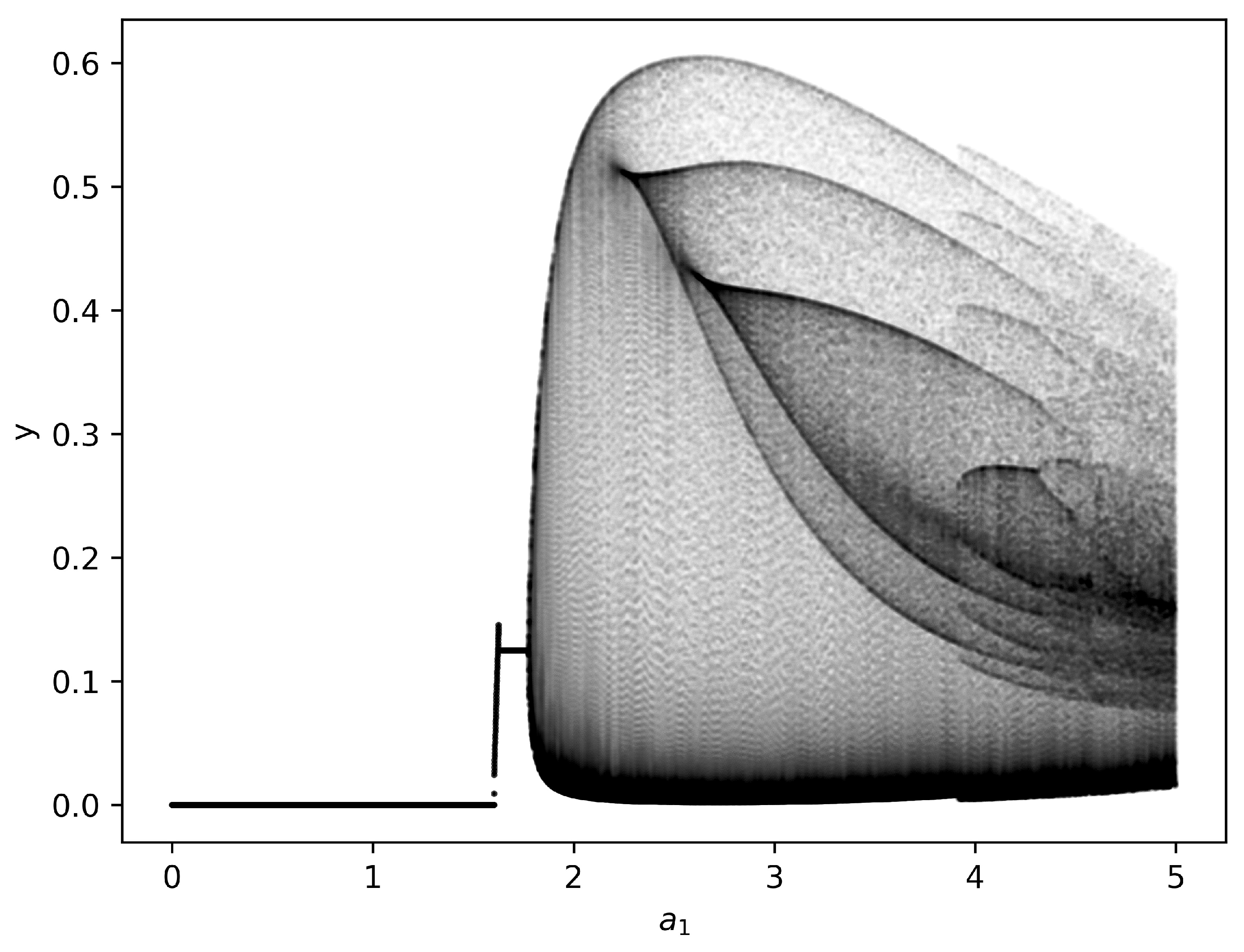
Figure 3.
Duration of the off (laminar) phases of the x (dashed) and y (solid) components with a stochastic parameter in the Hastings–Powell model. The dotted line indicates a dependence proportional to .
Figure 3.
Duration of the off (laminar) phases of the x (dashed) and y (solid) components with a stochastic parameter in the Hastings–Powell model. The dotted line indicates a dependence proportional to .
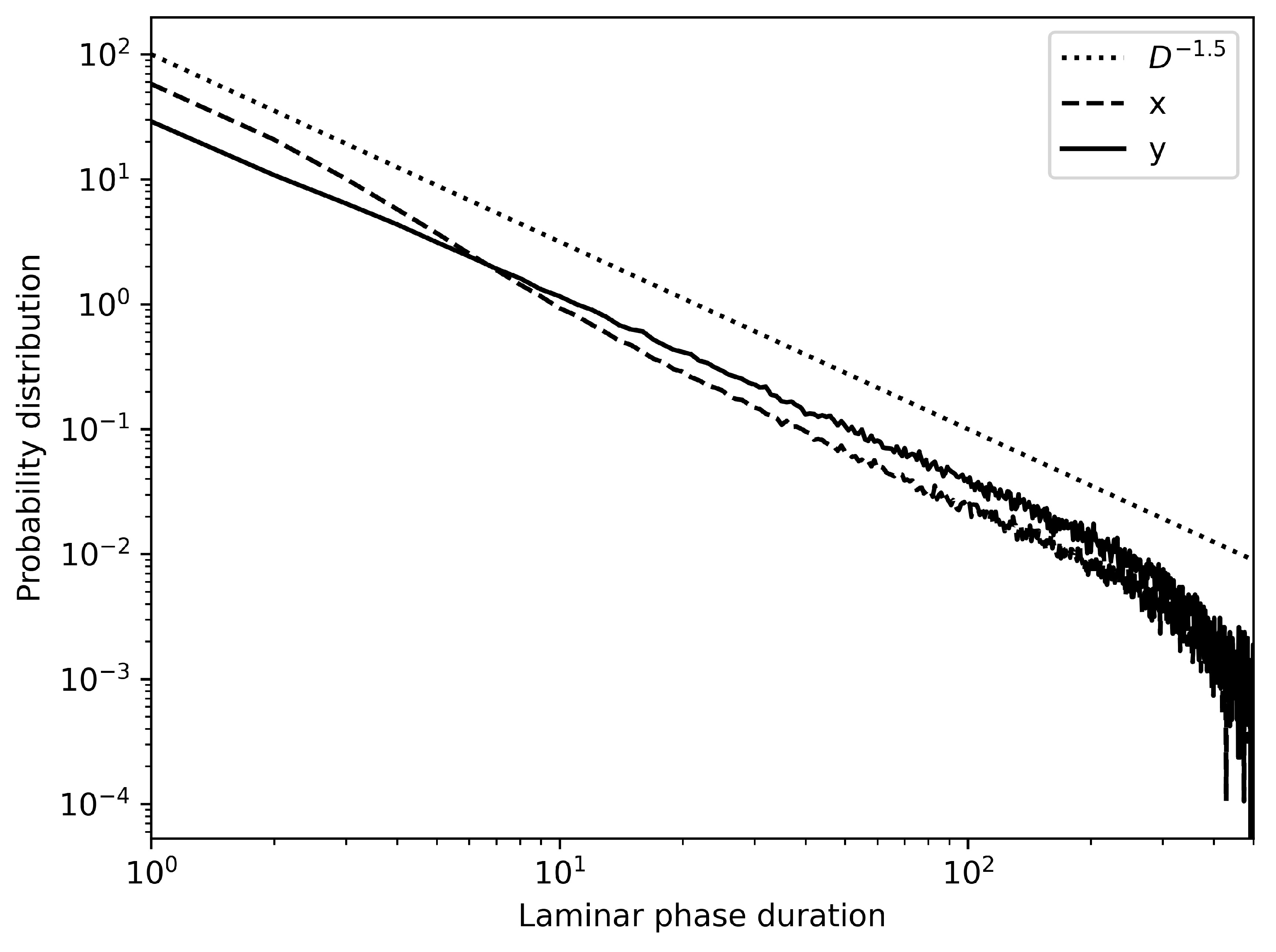
Figure 4.
Probability distribution of the maxima of (Panel a), y (Panel b), z (Panel c), in case of non-intermittent dynamics (solid line) and for on–off intermittent behavior (dotted line).
Figure 4.
Probability distribution of the maxima of (Panel a), y (Panel b), z (Panel c), in case of non-intermittent dynamics (solid line) and for on–off intermittent behavior (dotted line).
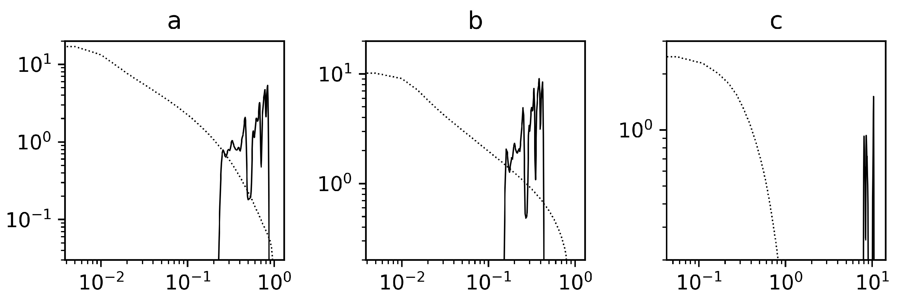
Figure 5.
Stochastic with . Time series of x (Panel a), y (Panel b) and of the running mean of the random variable controlling , computed on a window with width —the dotted line is the mean value of (Panel d). The probability distributions of the maxima of and y are shown in (Panel c).
Figure 5.
Stochastic with . Time series of x (Panel a), y (Panel b) and of the running mean of the random variable controlling , computed on a window with width —the dotted line is the mean value of (Panel d). The probability distributions of the maxima of and y are shown in (Panel c).
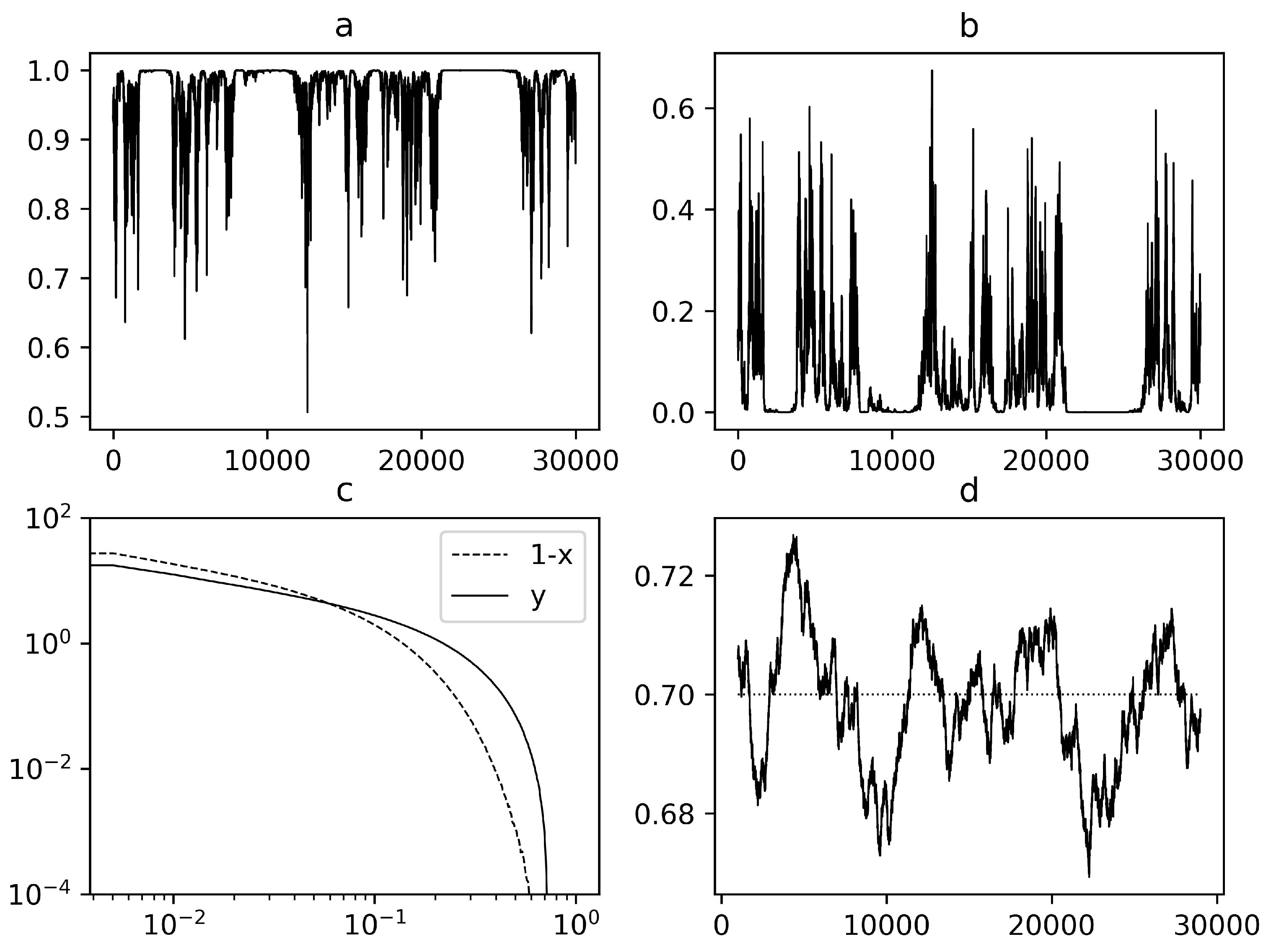
Figure 6.
Laminar phase duration of the x (dashed) and y (solid) variables for stochastic variability of the carrying capacity in the case . The dotted line is proportional to .
Figure 6.
Laminar phase duration of the x (dashed) and y (solid) variables for stochastic variability of the carrying capacity in the case . The dotted line is proportional to .
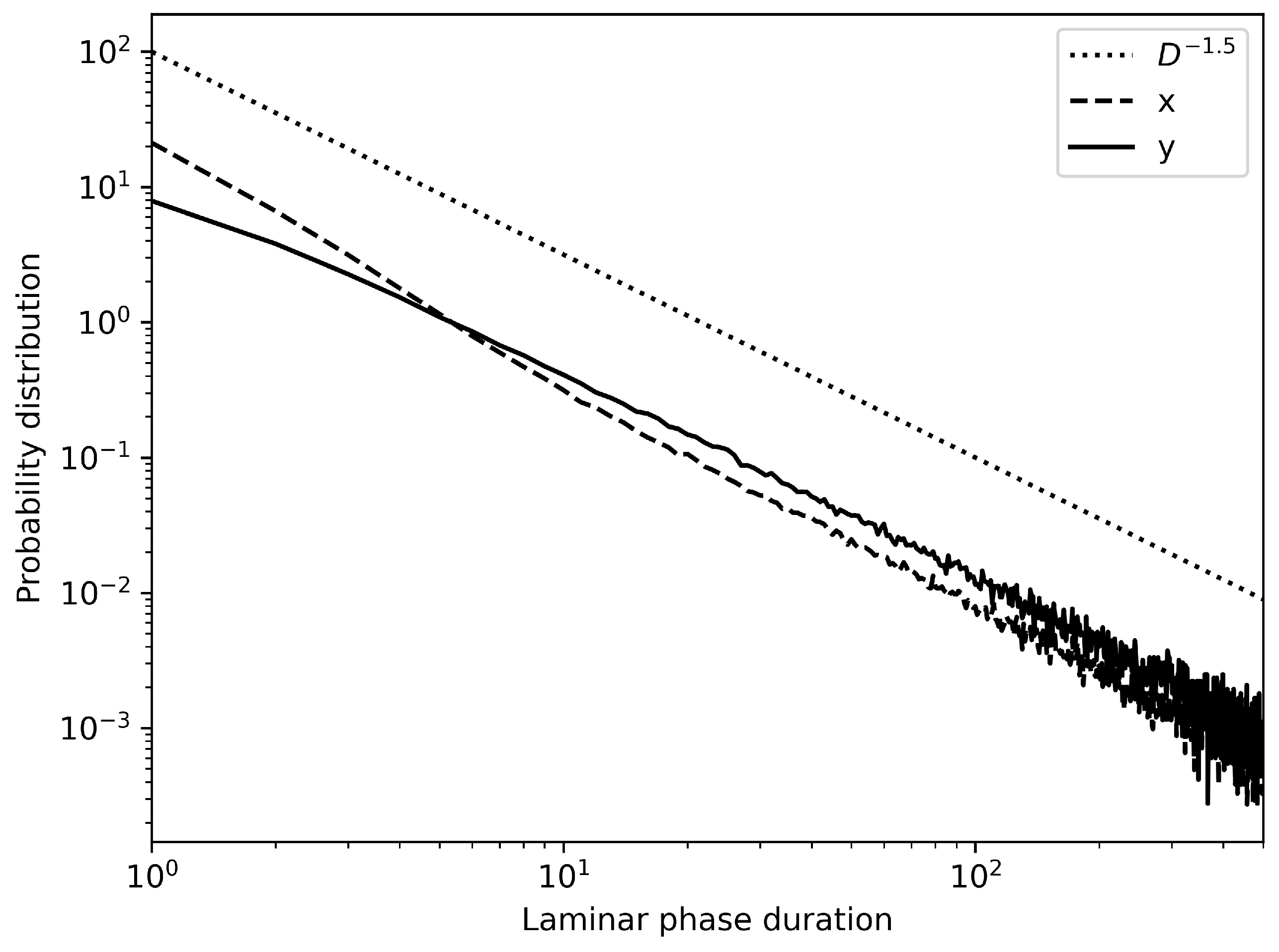
Figure 7.
(Left panel) Time series of z in the case ; (Right panel) Laminar phase durations of the predator/parasitoid z (solid) for stochastic with . The dashed line is proportional to .
Figure 7.
(Left panel) Time series of z in the case ; (Right panel) Laminar phase durations of the predator/parasitoid z (solid) for stochastic with . The dashed line is proportional to .
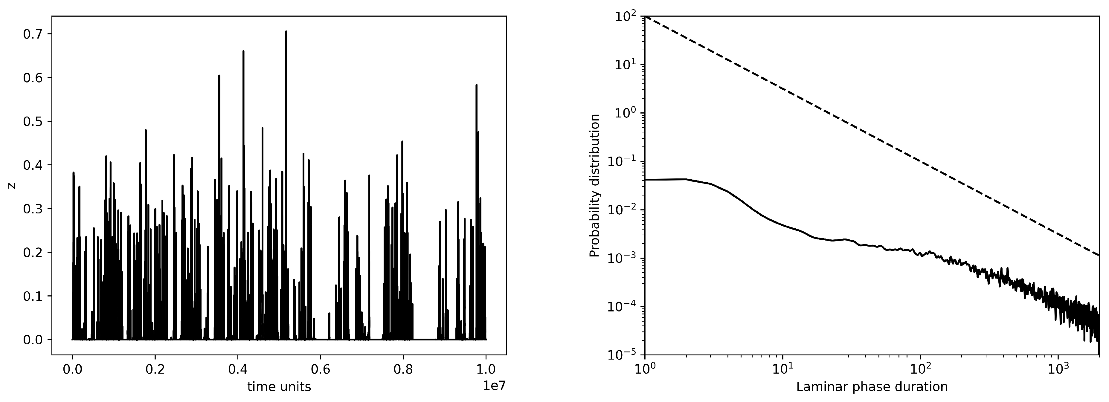
Figure 8.
(Left panel) Time series of y in case ; (Right panel) Laminar phase durations of the x (dashed) and y (solid) variables for stochastic with . The dotted line is proportional to .
Figure 8.
(Left panel) Time series of y in case ; (Right panel) Laminar phase durations of the x (dashed) and y (solid) variables for stochastic with . The dotted line is proportional to .
Publisher’s Note: MDPI stays neutral with regard to jurisdictional claims in published maps and institutional affiliations. |
© 2021 by the authors. Licensee MDPI, Basel, Switzerland. This article is an open access article distributed under the terms and conditions of the Creative Commons Attribution (CC BY) license (https://creativecommons.org/licenses/by/4.0/).
Share and Cite
MDPI and ACS Style
Vissio, G.; Provenzale, A. On-Off Intermittency in a Three-Species Food Chain. Mathematics 2021, 9, 1641. https://doi.org/10.3390/math9141641
AMA Style
Vissio G, Provenzale A. On-Off Intermittency in a Three-Species Food Chain. Mathematics. 2021; 9(14):1641. https://doi.org/10.3390/math9141641
Chicago/Turabian StyleVissio, Gabriele, and Antonello Provenzale. 2021. "On-Off Intermittency in a Three-Species Food Chain" Mathematics 9, no. 14: 1641. https://doi.org/10.3390/math9141641
Note that from the first issue of 2016, this journal uses article numbers instead of page numbers. See further details here.