
AutoNowP: An Approach Using Deep Autoencoders for Precipitation Nowcasting Based on Weather Radar Reflectivity Prediction

 and
and
Abstract
:1. Introduction
- RQ1
- How to use an ensemble of ConvAEs to supervisedly discriminate between severe and normal rainfall conditions, considering the encoded relationships between radar products values corresponding to both normal and severe weather events?
- RQ2
- What is the performance of introduced for answering RQ1 on real radar data collected from Romania and Norway and how does it compare to similar related work?
2. Literature Review on Machine-Learning-Based Precipitation Nowcasting
3. Methodology
3.1. Data Representation and Preprocessing
- is the value of at time t and location l;
- is the normalized value of at time t and location l;
- is the minimum value in the domain of ;
- is the maximum value in the domain of .
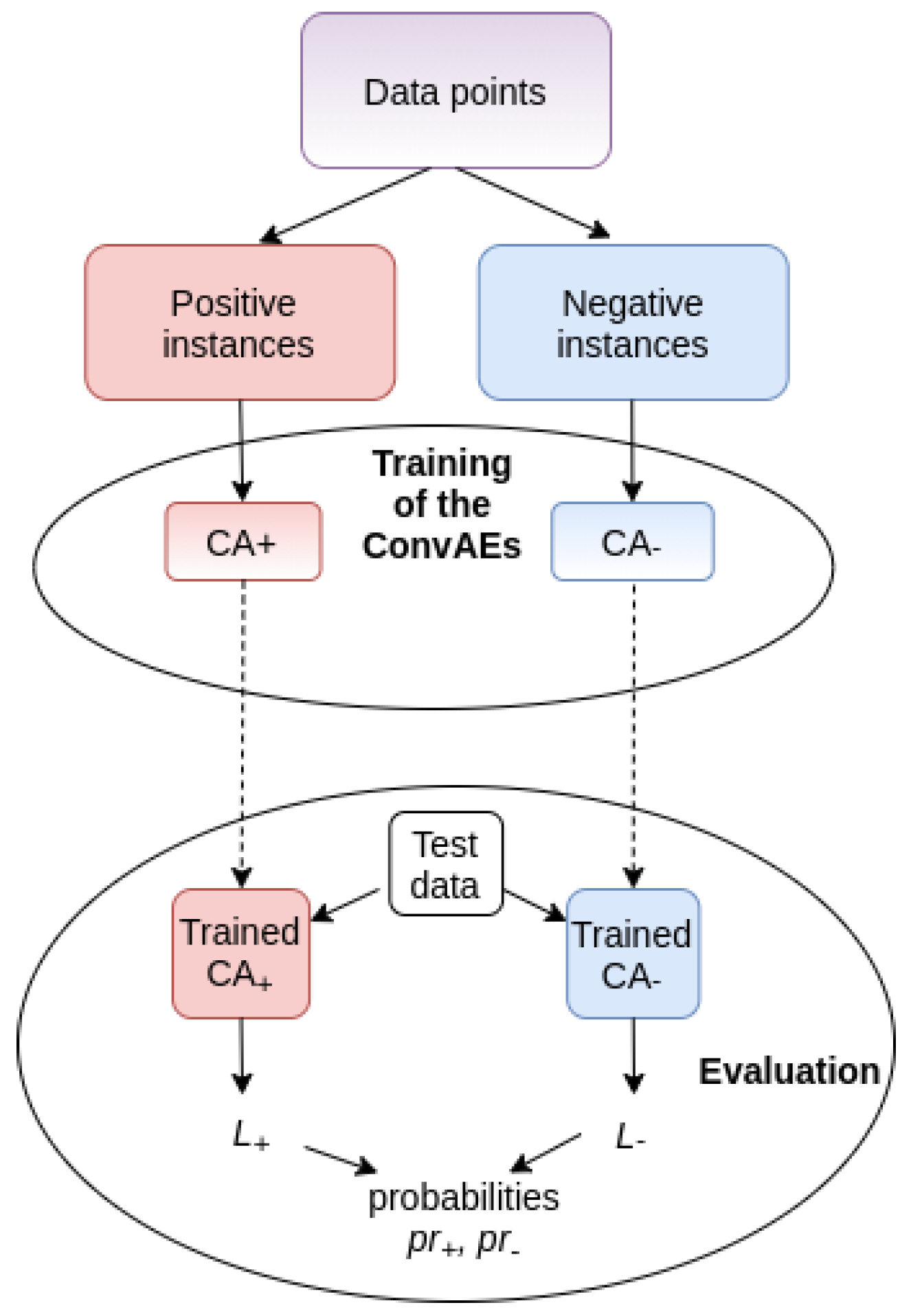
3.2. Classification Model
3.2.1. Training
Autoencoders Architecture
Loss Functions
- d is the diameter of the neighborhood used for characterizing the input instances x (see Section 4.1);
- is the -dimensional instance for which we compute the loss;
- is the autoencoder output for instance x (the reconstruction of x);
- is the chosen threshold that differentiates between positive and negative class;
- is the parameter that we introduced for the loss;
- and denote the ith component from x and respectively.
3.2.2. Classification Using
- if (and consequently ) it follows that ;
- increases as decreases;
- if , then , meaning that q is classified by as being negative.
3.3. Testing
- 1.
- Critical success index () computed as is used for convective storms nowcasting based on radar data [30].
- 2.
- True skill statistic (), .
- 3.
- Probability of detection (), also known as sensitivity or recall, is the true positive rate (TPRate), .
- 4.
- Precision for the positive class, also known as positive predictive value (), .
- 5.
- Precision for the negative class, also known as negative predictive value (), .
- 6.
- Specificity (), also known as true negative rate (TNRate), .
- 7.
- Area Under the ROC Curve (). The measure is recommended in case of imbalanced data and is computed as the average between the true positive rate and the true negative rate, .
- 8.
- Area Under the Precision–Recall Curve (), computed as the average between the precision and recall values, .
4. Data and Experiments
4.1. Data Sets
4.1.1. NMA Radar Data Set
4.1.2. MET Radar Data Set
4.2. Results
5. Discussion
5.1. Analysis of performance
5.2. Comparison to Related Work
6. Conclusions and Future Work
Author Contributions
Funding
Institutional Review Board Statement
Informed Consent Statement
Data Availability Statement
Acknowledgments
Conflicts of Interest
References
- Chen, L.; Cao, Y.; Ma, L.; Zhang, J. A Deep Learning-Based Methodology for Precipitation Nowcasting With Radar. Earth Space Sci. 2020, 7, e2019EA000812. [Google Scholar] [CrossRef] [Green Version]
- Jongman, B. Effective adaptation to rising flood risk. Nat. Commun. 2018, 9, 1–3. [Google Scholar] [CrossRef] [Green Version]
- Arnell, N.; Gosling, S. The impacts of climate change on river flood risk at the global scale. Clim. Chang. 2016, 134, 387–401. [Google Scholar] [CrossRef] [Green Version]
- Silvertown, J. A new dawn for citizen science. Trends Ecol. Evol. 2009, 24, 467–471. [Google Scholar] [CrossRef] [PubMed]
- Dixon, M.; Wiener, G. TITAN: Thunderstorm Identification, Tracking, Analysis, and Nowcasting—A radar-based methodology. J. Atmos. Ocean. Technol. 1993, 10, 785–797. [Google Scholar] [CrossRef]
- Johnson, J.T.; MacKeen, P.L.; Witt, A.; Mitchell, E.D.W.; Stumpf, G.J.; Eilts, M.D.; Thomas, K.W. The Storm Cell Identification and Tracking Algorithm: An Enhanced WSR-88D Algorithm. Weather Forecast. 1998, 13, 263–276. [Google Scholar] [CrossRef] [Green Version]
- Haiden, T.; Kann, A.; Wittmann, C.; Pistotnik, G.; Bica, B.; Gruber, C. The Integrated Nowcasting through Comprehensive Analysis (INCA) System and Its Validation over the Eastern Alpine Region. Weather Forecast. 2011, 26, 166–183. [Google Scholar] [CrossRef]
- Sun, J.; Xue, M.; Wilson, J.W.; Zawadzki, I.; Ballard, S.; Onvlee-HooiMeyer, J.; Joe, P.; Barker, D.; Li, P.W.; Golding, B.; et al. Use of NWP for Nowcasting Convective Precipitation: Recent Progress and Challenges. Bull. Am. Meteorol. Soc. 2014, 95, 409–426. [Google Scholar] [CrossRef] [Green Version]
- Han, L.; Sun, J.; Zhang, W. Convolutional Neural Network for Convective Storm Nowcasting Using 3D Doppler Weather Radar Data. arXiv 2019, arXiv:1911.06185. [Google Scholar]
- Tan, C.; Feng, X.; Long, J.; Geng, L. FORECAST-CLSTM: A New Convolutional LSTM Network for Cloudage Nowcasting. In Proceedings of the 2018 IEEE Visual Communications and Image Processing (VCIP), Taichung, Taiwan, 10–12 December 2018; pp. 1–4. [Google Scholar]
- Czibula, G.; Mihai, A.; Czibula, I.G. RadRAR: A relational association rule mining approach for nowcasting based on predicting radar products’ values. Procedia Comput. Sci. 2020, 176, 300–309. [Google Scholar] [CrossRef]
- Hao, L.; Kim, J.; Kwon, S.; Ha, I.D. Deep Learning-Based Survival Analysis for High-Dimensional Survival Data. Mathematics 2021, 9, 1244. [Google Scholar] [CrossRef]
- Mousavi, S.M.; Ghasemi, M.; Dehghan Manshadi, M.; Mosavi, A. Deep Learning for Wave Energy Converter Modeling Using Long Short-Term Memory. Mathematics 2021, 9, 871. [Google Scholar] [CrossRef]
- Castorena, C.M.; Abundez, I.M.; Alejo, R.; Granda-Gutiérrez, E.E.; Rendón, E.; Villegas, O. Deep Neural Network for Gender-Based Violence Detection on Twitter Messages. Mathematics 2021, 9, 807. [Google Scholar] [CrossRef]
- Sønderby, C.K.; Espeholt, L.; Heek, J.; Dehghani, M.; Oliver, A.; Salimans, T.; Hickey, J.; Agrawal, S.; Kalchbrenner, N. MetNet: A Neural Weather Model for Precipitation Forecasting. arXiv 2020, arXiv:2003.12140. [Google Scholar]
- Alain, G.; Bengio, Y. What regularized auto-encoders learn from the data-generating distribution. J. Mach. Learn. Res. 2014, 15, 3563–3593. [Google Scholar]
- Trebing, K.; Stanczyk, T.; Mehrkanoon, S. SmaAt-UNet: Precipitation nowcasting using a small attention-UNet architecture. Pattern Recognit. Lett. 2021, 145, 178–186. [Google Scholar] [CrossRef]
- Tekin, S.F.; Karaahmetoglu, O.; Ilhan, F.; Balaban, I.; Kozat, S.S. Spatio-temporal Weather Forecasting and Attention Mechanism on Convolutional LSTMs. arXiv 2021, arXiv:2102.00696. [Google Scholar]
- Shi, X.; Chen, Z.; Wang, H.; Yeung, D.Y.; Wong, W.k.; Woo, W.c. Convolutional LSTM Network: A ML Approach for Precipitation Nowcasting. In Proceedings of the 28th International Conference on Neural Information Processing Systems, Montreal, QC, Canada, 7–12 December 2015; MIT Press: Cambridge, UK, 2015; Volume 1, pp. 802–810. [Google Scholar]
- Heye, A.; Venkatesan, K.; Cain, J. Precipitation Nowcasting: Leveraging Deep Convolutional Recurrent Neural Networks. In Proceedings of the 31st Conference on Neural Information Processing Systems, Long Beach, NY, USA, 4–9 December 2017; pp. 1–8. [Google Scholar]
- Tian, L.; Li, X.; Ye, Y.; Xie, P.; Li, Y. A Generative Adversarial Gated Recurrent Unit Model for Precipitation Nowcasting. IEEE Geosci. Remote Sens. Lett. 2020, 17, 601–605. [Google Scholar] [CrossRef]
- Han, L.; Sun, J.; Zhang, W. Convolutional Neural Network for Convective Storm Nowcasting Using 3-D Doppler Weather Radar Data. IEEE Trans. Geosci. Remote Sens. 2020, 58, 1487–1495. [Google Scholar] [CrossRef]
- Franch, G.; Nerini, D.; Pendesini, M.; Coviello, L.; Jurman, G.; Furlanello, C. Precipitation Nowcasting with Orographic Enhanced Stacked Generalization: Improving Deep Learning Predictions on Extreme Events. Atmosphere 2020, 11, 267. [Google Scholar] [CrossRef] [Green Version]
- Jeong, C.H.; Kim, W.; Joo, W.; Jang, D.; Yi, M.Y. Enhancing the Encoding-Forecasting Model for Precipitation Nowcasting by Putting High Emphasis on the Latest Data of the Time Step. Atmosphere 2021, 12, 261. [Google Scholar] [CrossRef]
- Yo, T.S.; Su, S.H.; Chu, J.L.; Chang, C.W.; Kuo, H.C. A Deep Learning Approach to Radar-Based QPE. Earth Space Sci. 2021, 8, e2020EA001340. [Google Scholar] [CrossRef]
- Mihai, A.; Czibula, G.; Mihulet, E. Analyzing Meteorological Data Using Unsupervised Learning Techniques. In Proceedings of the ICCP 2019: IEEE 15th International Conference on Intelligent Computer Communication and Processing, Cluj-Napoca, Romania, 5–7 September 2019; IEEE Computer Society: Washington, DC, USA, 2019; pp. 529–536. [Google Scholar]
- Klambauer, G.; Unterthiner, T.; Mayr, A.; Hochreiter, S. Self-Normalizing Neural Networks. In Proceedings of the 31st Conference on Neural Information Processing Systems, Long Beach, NY, USA, 4–9 December 2017; pp. 972–981. [Google Scholar]
- Kingma, D.P.; Ba, J. Adam: A Method for Stochastic Optimization. arXiv 2017, arXiv:1412.6980. [Google Scholar]
- Gu, Q.; Zhu, L.; Cai, Z. Evaluation Measures of the Classification Performance of Imbalanced Data Sets. In Computational Intelligence and Intelligent Systems; Springer: Berlin/Heidelberg, Germany, 2009; pp. 461–471. [Google Scholar]
- Czibula, G.; Mihai, A.; Mihuleţ, E. NowDeepN: An Ensemble of Deep Learning Models for Weather Nowcasting Based on Radar Products’ Values Prediction. Appl. Sci. 2021, 11, 125. [Google Scholar] [CrossRef]
- Brown, L.; Cat, T.; DasGupta, A. Interval Estimation for a proportion. Stat. Sci. 2001, 16, 101–133. [Google Scholar] [CrossRef]
- MET Norway Thredds Data Server. Available online: https://thredds.met.no/thredds/catalog.html (accessed on 7 May 2021).
- Composite Reflectivity Product—MET Norway Thredds Data Server. Available online: https://thredds.met.no/thredds/catalog/remotesensing/reflectivity-nordic/catalog.html (accessed on 15 May 2021).
- Sekerka, R.F. 15—Entropy and Information Theory. In Thermal Physics; Sekerka, R.F., Ed.; Elsevier: Amsterdam, The Netherlands, 2015; pp. 247–256. [Google Scholar]
- Jolliffe, I.T.; Cadima, J. Principal component analysis: A review and recent developments. Philos. Trans. R. Soc. A Math. Phys. Eng. Sci. 2016, 374, 20150202. [Google Scholar] [CrossRef]
- NMA Data Set. Available online: http://www.cs.ubbcluj.ro/~mihai.andrei/datasets/autonowp/ (accessed on 15 May 2021).
- MET Data Set. Available online: https://thredds.met.no/thredds/catalog/remotesensing/reflectivity-nordic/2019/05/catalog.html?dataset=remotesensing/reflectivity-nordic/2019/05/yrwms-nordic.mos.pcappi-0-dbz.noclass-clfilter-novpr-clcorr-block.laea-yrwms-1000.20190522.nc (accessed on 15 May 2021).
- Keras. The Python Deep Learning Library. 2018. Available online: https://keras.io/ (accessed on 15 May 2021).
- Han, L.; Sun, J.; Zhang, W.; Xiu, Y.; Feng, H.; Lin, Y. A machine learning nowcasting method based on real-time reanalysis data. J. Geophys. Res. Atmos. 2017, 122, 4038–4051. [Google Scholar] [CrossRef]
- Tran, Q.K.; Song, S.K. Computer Vision in Precipitation Nowcasting: Applying Image Quality Assessment Metrics for Training Deep Neural Networks. Atmosphere 2019, 10, 244. [Google Scholar] [CrossRef] [Green Version]
- Scikit-Learn. Machine Learning in Python. 2021. Available online: http://scikit-learn.org/stable/ (accessed on 1 May 2021).
- Mel, R.A.; Viero, D.P.; Carniello, L.; D’Alpaos, L. Optimal floodgate operation for river flood management: The case study of Padova (Italy). J. Hydrol. Reg. Stud. 2020, 30, 100702. [Google Scholar] [CrossRef]


| Data Set | Product of Interest () | # Instances | % of “+” Instances | % of “−” Instances | Entropy |
|---|---|---|---|---|---|
| NMA | R01 | 9003688 | 3.44% | 96.56% | 0.216 |
| MET | Composite reflectivity | 6607836 | 31.97% | 68.03% | 0.904 |
| Data Set | |||||||||
|---|---|---|---|---|---|---|---|---|---|
| 0.615 | 0.861 | 0.876 | 0.674 | 0.996 | 0.985 | 0.931 | 0.775 | ||
| 10 | ± | ± | ± | ± | ± | ± | ± | ± | |
| 0.018 | 0.012 | 0.012 | 0.017 | 0.001 | 0.002 | 0.006 | 0.013 | ||
| 0.425 | 0.471 | 0.474 | 0.810 | 0.989 | 0.997 | 0.736 | 0.642 | ||
| NMA | 20 | ± | ± | ± | ± | ± | ± | ± | ± |
| 0.072 | 0.091 | 0.092 | 0.015 | 0.001 | 0.001 | 0.046 | 0.039 | ||
| 0.151 | 0.157 | 0.157 | 0.812 | 0.993 | 1.000 | 0.579 | 0.485 | ||
| 30 | ± | ± | ± | ± | ± | ± | ± | ± | |
| 0.046 | 0.051 | 0.028 | 0.031 | 0.001 | 0.000 | 0.014 | 0.007 | ||
| 0.681 | 0.740 | 0.872 | 0.757 | 0.936 | 0.867 | 0.870 | 0.814 | ||
| 10 | ± | ± | ± | ± | ± | ± | ± | ± | |
| 0.014 | 0.009 | 0.019 | 0.027 | 0.005 | 0.026 | 0.005 | 0.008 | ||
| 0.566 | 0.626 | 0.675 | 0.793 | 0.920 | 0.951 | 0.813 | 0.734 | ||
| MET | 15 | ± | ± | ± | ± | ± | ± | ± | ± |
| 0.05 | 0.09 | 0.12 | 0.08 | 0.03 | 0.03 | 0.05 | 0.029 | ||
| 0.401 | 0.500 | 0.536 | 0.710 | 0.947 | 0.963 | 0.750 | 0.623 | ||
| 20 | ± | ± | ± | ± | ± | ± | ± | ± | |
| 0.090 | 0.223 | 0.269 | 0.173 | 0.026 | 0.046 | 0.111 | 0.048 |
| Value | 0.364 | 0.439 | 0.463 | 0.641 | 0.953 | 0.976 | 0.719 | 0.552 |
| ± | ± | ± | ± | ± | ± | ± | ± | |
| 95% CI | 0.035 | 0.072 | 0.084 | 0.050 | 0.003 | 0.012 | 0.036 | 0.018 |
| Improvement | 69% | 96% | 89% | 5% | 4% | 1% | 29% | 40% |
| Data Set | Model | ||||||||
|---|---|---|---|---|---|---|---|---|---|
| 0.615 | 0.861 | 0.876 | 0.674 | 0.996 | 0.985 | 0.931 | 0.775 | ||
| AutoNowP | ± | ± | ± | ± | ± | ± | ± | ± | |
| 0.018 | 0.012 | 0.012 | 0.017 | 0.001 | 0.002 | 0.006 | 0.013 | ||
| 0.672 | 0.752 | 0.757 | 0.857 | 0.992 | 0.996 | 0.876 | 0.807 | ||
| LR | ± | ± | ± | ± | ± | ± | ± | ± | |
| 0.012 | 0.013 | 0.013 | 0.005 | 0.001 | 0.000 | 0.007 | 0.008 | ||
| 0.685 | 0.778 | 0.783 | 0.845 | 0.992 | 0.995 | 0.889 | 0.814 | ||
| NMA | Linear SVC | ± | ± | ± | ± | ± | ± | ± | ± |
| 0.012 | 0.007 | 0.007 | 0.015 | 0.000 | 0.000 | 0.003 | 0.009 | ||
| 0.574 | 0.725 | 0.734 | 0.724 | 0.991 | 0.990 | 0.862 | 0.729 | ||
| DT | ± | ± | ± | ± | ± | ± | ± | ± | |
| 0.007 | 0.004 | 0.006 | 0.012 | 0.001 | 0.002 | 0.002 | 0.006 | ||
| 0.571 | 0.793 | 0.807 | 0.662 | 0.993 | 0.986 | 0.896 | 0.735 | ||
| NCC | ± | ± | ± | ± | ± | ± | ± | ± | |
| 0.006 | 0.013 | 0.013 | 0.015 | 0.001 | 0.001 | 0.006 | 0.003 | ||
| 0.681 | 0.740 | 0.872 | 0.757 | 0.936 | 0.867 | 0.870 | 0.814 | ||
| AutoNowP | ± | ± | ± | ± | ± | ± | ± | ± | |
| 0.014 | 0.009 | 0.019 | 0.027 | 0.005 | 0.026 | 0.005 | 0.008 | ||
| 0.760 | 0.796 | 0.853 | 0.875 | 0.932 | 0.943 | 0.898 | 0.864 | ||
| LR | ± | ± | ± | ± | ± | ± | ± | ± | |
| 0.006 | 0.002 | 0.001 | 0.007 | 0.003 | 0.002 | 0.001 | 0.004 | ||
| 0.761 | 0.798 | 0.858 | 0.870 | 0.934 | 0.940 | 0.899 | 0.864 | ||
| MET | Linear SVC | ± | ± | ± | ± | ± | ± | ± | ± |
| 0.006 | 0.002 | 0.001 | 0.007 | 0.003 | 0.003 | 0.001 | 0.004 | ||
| 0.670 | 0.710 | 0.804 | 0.801 | 0.908 | 0.906 | 0.855 | 0.803 | ||
| DT | ± | ± | ± | ± | ± | ± | ± | ± | |
| 0.010 | 0.004 | 0.005 | 0.009 | 0.003 | 0.002 | 0.002 | 0.007 | ||
| 0.681 | 0.728 | 0.831 | 0.791 | 0.919 | 0.897 | 0.864 | 0.811 | ||
| NCC | ± | ± | ± | ± | ± | ± | ± | ± | |
| 0.009 | 0.005 | 0.009 | 0.007 | 0.001 | 0.006 | 0.003 | 0.007 |
| NMA Data | MET Data | Total | |
|---|---|---|---|
| WIN | 21 | 16 | 37 |
| LOSE | 11 | 16 | 27 |
| % WIN | 66% | 50% | 58% |
Publisher’s Note: MDPI stays neutral with regard to jurisdictional claims in published maps and institutional affiliations. |
© 2021 by the authors. Licensee MDPI, Basel, Switzerland. This article is an open access article distributed under the terms and conditions of the Creative Commons Attribution (CC BY) license (https://creativecommons.org/licenses/by/4.0/).
Share and Cite
Czibula, G.; Mihai, A.; Albu, A.-I.; Czibula, I.-G.; Burcea, S.; Mezghani, A. AutoNowP: An Approach Using Deep Autoencoders for Precipitation Nowcasting Based on Weather Radar Reflectivity Prediction. Mathematics 2021, 9, 1653. https://doi.org/10.3390/math9141653
Czibula G, Mihai A, Albu A-I, Czibula I-G, Burcea S, Mezghani A. AutoNowP: An Approach Using Deep Autoencoders for Precipitation Nowcasting Based on Weather Radar Reflectivity Prediction. Mathematics. 2021; 9(14):1653. https://doi.org/10.3390/math9141653
Chicago/Turabian StyleCzibula, Gabriela, Andrei Mihai, Alexandra-Ioana Albu, Istvan-Gergely Czibula, Sorin Burcea, and Abdelkader Mezghani. 2021. "AutoNowP: An Approach Using Deep Autoencoders for Precipitation Nowcasting Based on Weather Radar Reflectivity Prediction" Mathematics 9, no. 14: 1653. https://doi.org/10.3390/math9141653
APA StyleCzibula, G., Mihai, A., Albu, A.-I., Czibula, I.-G., Burcea, S., & Mezghani, A. (2021). AutoNowP: An Approach Using Deep Autoencoders for Precipitation Nowcasting Based on Weather Radar Reflectivity Prediction. Mathematics, 9(14), 1653. https://doi.org/10.3390/math9141653