Abstract
The main target of this research work is to model the output performance of adsorption water desalination system (AWDS) in terms of switching and cycle time using artificial intelligence. The output performance of the ADC system is expressed by the specific daily water production (SDWP), the coefficient of performance (COP), and specific cooling power (SCP). A robust Adaptive Network-based Fuzzy Inference System (ANFIS) model of SDWP, COP, and SCP was built using the measured data. To demonstrate the superiority of the suggested ANFIS model, the model results were compared with those achieved by Analysis of Variance (ANOVA) based on the maximum coefficient of determination and minimum error between measured and estimated data in addition to the mean square error (MSE). Applying ANOVA, the average coefficient-of-determination values were 0.8872 and 0.8223, respectively, for training and testing. These values are increased to 1.0 and 0.9673, respectively, for training and testing thanks to ANFIS based modeling. In addition, ANFIS modelling decreased the RMSE value of all datasets by 83% compared with ANOVA. In sum, the main findings confirmed the superiority of ANFIS modeling of the output performance of adsorption water desalination system compared with ANOVA.
1. Introduction
It has become evident that the energy and water dilemmas are escalating day by day to the point where they threaten the lives of many people and fuel conflicts between societies [1]. And that the two problems have become so intertwined that they cannot be separated, because if you want to save water, you must consume the scarce energy in the first place. It is also noticeable that the areas that suffer from severe water shortages are mostly desert areas and have untapped solar energy available [2]. Therefore, researchers in this field should think about how to link the parties to this puzzle and use that wasted energy to provide the required water, especially in light of the availability of seawater and wells that are not suitable for drinking [3]. The researchers have improved in this way and made a great effort until they presented many ideas that can be built upon and developed. Among these ideas was the idea to use the phenomenon of adsorption to desalinate water with solar energy or waste energy. This idea went through many stages until prototypes were built and work was carried out to improve its performance in several ways, including improving the properties of the used materials. One of these methods is to improve the properties of the used materials, and also to improve the working cycle and try to make it work efficiently at lower temperatures, which was a great challenge. The strength of adsorption desalination systems is that they are suitable for being run with solar energy or waste energy, but they have a weak point, which is their low productivity compared to widespread systems such as reverse osmosis systems (RO) [4]. Hence, researches were conducted theoretically and experimentally on improving and promoting the system performance. Different ways of researches had been followed like presenting new adsorbents and merging this technology with others like RO. Among these research ways were attempts to improve the performance by controlling cycle time and heating and cooling times.
Heat recovery has been presented by Ng et al. [5] between evaporator and condenser to produce a SDWP of about 27 m3/ton per day of silica gel every day. Also, heat recovery between the adsorption beds has been examined by Ma et al. [6] reaching SDWP 4.69 m3/ton of silica gel and COP of 0.766. Four adsorption beds connected to two evaporators have been studied theoretically by Ali et al. [7]. SDWP of 8.84 m3/ton/day has been reached in this study at a COP of 0.52 employing 95 °C driving temperature. At 80 °C driving temperature, the AD cycle showed its ability to be work as shown by Olkis et al. [8] experimentally where the studied AD system produced a SDWP of 10.9 m3/ton/day. The effect of the temperatures of the condenser and the evaporator on the AD productivity has been studied numerically by Youssef et al. [9] to optimize the system performance. SDWP of 10 m3/ton/day has been recorded at a condenser temperature of 10 °C and an evaporator temperature of 30 °C.
Using heat and mass recovery, the performance of a 2-bed AD system has been studied by Amirfakhraei et al. [10]. The theoretical study showed that the cycle could reach a SDWP of 9.58 m3/ton of silica gel daily by using heating and cooling temperatures of 95 °C and 30 °C, respectively. Zhang et al. [11] presented an experimental optimization study for an AD system by operating conditions. Desalinated water of 191.3 kg/h has been reached at a heating temperature of 80 °C. Another optimization study has been presented by Rezk et al. [12] using a model optimization method to declare the optimal operating conditions of solar-driven AD cycle. The optimal cycle could produce a SDWP of about 6.9 m3/ton silica gel/day, a SCP of 191 W/kg, and a COP of 0.961.
Based on the above, it becomes clear to us that many efforts are being made to improve and raise the performance of the adsorption desalination systems; however, these efforts must be continued. It is worth mentioning here that there is something that can be added in this area if the operating cycle is well examined and modeled to extract the highest possible productivity without changing the construction or the content of the system, only by reaching the best-operating conditions. The model has been presented here employing artificial intelligence (AI) based on an experimental dataset to save money, effort, and time. Artificial intelligence tools conquered many fields of applications. Systems modeling is one of these fields [13,14]. The choice of the AI modeling tool depends mainly on the nature of the application and the available dataset. Fuzzy Logic (FL) and Artificial Neural Networks (ANN) are two popular and efficient AI techniques. Therefore, the main target of this research work is to model the output performance of adsorption water desalination system (AWDS) in terms of switching and cycle time using an Adaptive Network-based Fuzzy Inference System (ANFIS). The output performance of the SADC system is expressed by the specific daily water production (SDWP), the coefficient of performance (COP) and specific cooling power (SCP). A robust ANFIS model of SDWP, COP, and SCP was built using the measured data. To demonstrate the superiority of the suggested ANFIS model, the model results were compared with those achieved by Analysis of Variance (ANOVA) based on the maximum coefficient of determination and minimum error between measured and estimated data. AVOVA has been used in several applications such as a bioelectrochemical desalination process [15], biodesalination of Seawater [16] and desalination by reverse osmosis [17]. Therefore, it has been used as a benchmark for the problem under study.
2. Experimental Work
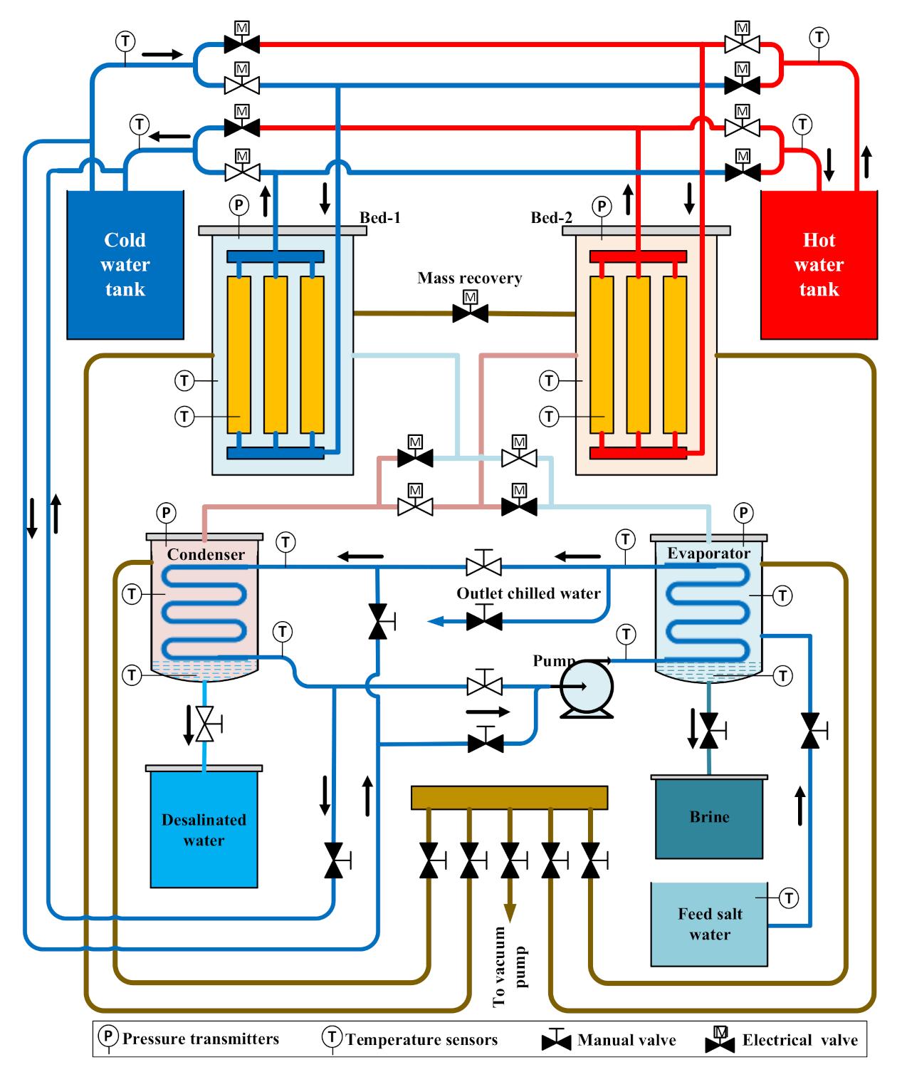
An adsorption water desalination system has been built of two adsorption beds containing metal-organic framework MOF (CPO-27(Ni)). The system has a condenser and evaporator as shown in Figure 1. The system works in a semi-continuous mode where Bed1 and Bed 2 work interchangeably. When Bed1 is in adsorption mode, Bed2 is in the desorption mode. During the adsorption mode, the bed is cooled down by using cold water and during the desorption mode, the bed has been heated up using hot water. This system has been presented elsewhere and it is still under review. The condenser and the evaporator are connected to perform internal heat recovery which improves the performance of the system by raising the produced desalinated water. The operating conditions such as driving temperature, cooling temperature, switching time, and cycle time have been studied.
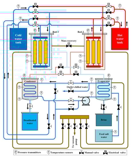
Figure 1.
Schematic diagram of the adsorption water desalination system.
3. Methodology
In this work, both ANOVA and ANFIS are considered. ANOVA is nominated in many experimental applications [15,16,17]. ANOVA mathematically quantifies the relationship between the output and inputs based on linear regression. The significance of every factor is considered based on its significant value, p-value. For input to be significant, its p-value must be lower than 5%.
ANFIS is featured with the advantages of FL and ANN. Modeling by ANFIS involves three phases. The first phase consists of fuzzifying the values of the input signals. This is performed by mapping the crisp values, through their corresponding membership functions (MFs), to fuzzy values. This phase is called fuzzification. These MFs can take either Gaussian or triangular shapes, depending on the application. The fuzzified inputs are logically processed to obtain the fuzzy output according to the pre-set fuzzy rules [14,18]. The second phase is the fuzzy inference system. In this phase, the fuzzy output is then passed to the defuzzification in order to return the output to its crisp values. There are two common methods of fuzzification: center of gravity and weighted average. Unlike mathematical modeling, which formulates the relation between the inputs and the corresponding output as a mathematical equation, fuzzy modeling describes this relationship via a set of IF (premise) THEN (consequence) rules. These rules are generally created based on experimental datasets. An example of a fuzzy rule statement, for a two-input single-output system, simply takes the form:
where MFa and MFb denote the fuzzy membership functions of the two inputs a and b, respectively, and MFc is the fuzzy membership function of the output c.
IF a is MFa and b is MFb, THEN c is MFc,
4. Results and Discussion
4.1. Modelling Based ANOVA
Table 1, Table 2 and Table 3 present the ANOVA results for modeling COP, SCP, and SDWP, respectively. Considering Table 1, for the first output response, the Model F-value of 60.33 implies the model is significant. There is only a 0.01% chance that an F-value this large could occur due to noise. The p-values less than 0.05 indicate model terms are significant. In this case A, A2 are significant model terms. Values greater than 0.1 indicate the model terms are not significant. The following relation in terms of actual factors can be used to make predictions about the first output response.

Table 1.
ANOVA table for first output response (COP).
Table 2.
ANOVA table for second output response (SCP).
Table 3.
ANOVA table for third output response (SDWP).
Regarding the second output response, the AVOVA data shown in Table 2, the Model F-value of 12.94 indicates the model is significant. There is only a 0.07% chance that an F-value this large could occur due to noise. The p-values less than 0.05 show model terms are significant. In this case, A, B, A2 are significant model terms. Values greater than 0.1000 indicate the model terms are not significant. The next relation in terms of actual factors can be used to make predictions about the second output response.
Regarding the third output response, the AVOVA data shown in Table 3, the Model F-value of 25.35 indicates the model is significant. There is only a 0.01% chance that an F-value this large could occur due to noise. The p-values less than 0.05 indicate model terms are significant. In this case A, A2 are significant model terms. Values greater than 0.1 indicate the model terms are not significant. The next relation in terms of actual factors can be used to make predictions about the second output response.
The statical analysis of different ANOVA models are presented in Table 4. For COP model, the predicted R2 of 0.9399 is in reasonable agreement with the adjusted R2 of 0.9549; i.e., the difference is less than 0.2. The value of RMSE is 0.6552. The adequate precision measures the signal to noise ratio. It compares the range of the predicted values at the design points to the average prediction error. Ratios greater than 4 indicate adequate model discrimination [19]. For COP model, the ratio of 20.228 indicates an adequate signal. This model can be used to navigate the design space.
Table 4.
Statical analysis of the ANOVA model.
For SCP, the predicted R2 of 0.6760 is in reasonable agreement with the adjusted R2 of 0.8100. The value of RMSE is 14.6263. Also, the adequate precision (11.675) is greater than 4 is desirable that indicates an adequate signal. This model can be used to navigate the design space. Finally, for SDWP, the predicted R2 of 0.8512 is in reasonable agreement with the adjusted R2 of 0.8969. The value of RMSE is 2.8071. The signal to noise of 13.826 indicates an adequate signal. This model can be used to navigate the design space. In sum, the average value of RMSE for the three models is 8.607.
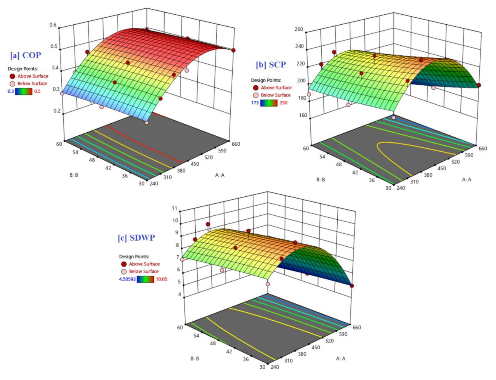
Figure 2 illustrates the 3-D surface plots for the three output response models. The red-filled circles show the response values above the predicted values, and the pink-filled circles show the values below the predicted one. The yellow curvature lines show the high output performances. As demonstrated in Figure 3, the actual values are the measured response, and the predicted response is determined by using the approximate function values to evaluate the model. Most of the results of both models are close to the diagonal, indicating an excellent correlation between the expected and the actual values.

Figure 2.
3-D response surface plots for output responses (a) COP; (b) SCP, and (c) SDWP.
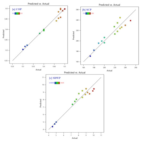
Figure 3.
Comparison of the predicted values of output response (a) COP; (b) SCP, and (c) SDWP.
4.2. Modelling Based ANFIS
Based on the experimental dataset, a model based ANFIS has been created to simulate the output performance of AWDS in terms of switching and cycle time. Three ANFIS models respectively for COP, SCP, and SDWP are created. The experimental dataset (15 experiments) was divided into two parts with a ratio of 70:30 for the training (10 experiments) and testing (5 experiments) stages. In the current model modeling, the Takagi-Sugeno ANFIS is adopted because of its ability to track the nonlinear data precisely. Also, the subtractive clustering method has been applied to build the fuzzy rules. The number of fuzzy rules is 9, 9, and 10, respectively, for COP, SCP, and SDWP. The minimum, maximum, and Wavg were used for the implication, aggregation, and defuzzification methods, respectively. Additionally, the inputs’ MFs were chosen as the Gaussian shape for the fuzzification procedure, and only 10 epochs were found to be enough for the training. The MSE, RMSE, and the coefficient of determination (R2) between the measured data and estimated data are used to evaluate the accuracy of the ANFIS model. The statistical assessment of the ANFIS models of COP, SCP, and SDWP is presented in Table 5. Applying ANOVA, the average coefficient-of-determination values were 0.8872 and 0.8223, respectively, for training and testing. These values are increased to 1.0 and 0.9673, respectively, for training and testing thanks to ANFIS based modeling. In addition, RMSE values using ANFIS were 0.00117, 2.5201 and 1.46 respectively, for training, testing and all datasets. Compared with ANOVA, the average RMSE value based on all datasets is decreased from 8.607 (ANOVA) to 1.46 by using ANFIS. This means ANFIS modelling decreased the RMSE of all datasets by 83% compared with ANOVA.
Table 5.
Statistical assessment of the ANFIS models of COP, SCP, and SDWP.
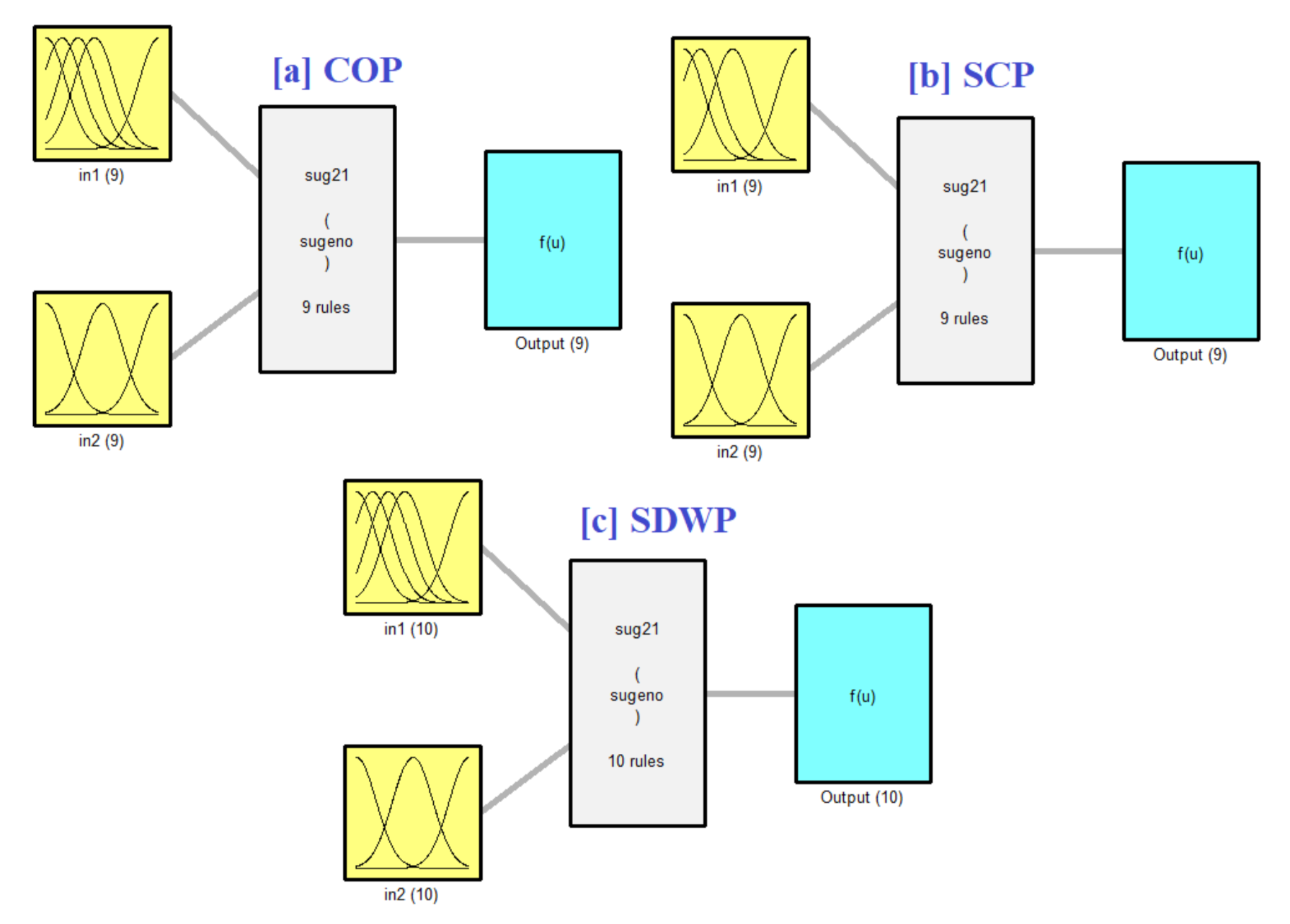
Figure 4 demonstrates the fuzzification phase in establishing an ANFIS model, in which the ANFIS model has two inputs (switching and cycle time) and one output for each model. The 3-D surface plot of the three output responses with varying input is shown in Figure 5. Whereas Figure 6. illustrates the input and the output membership functions of the fuzzy system for COP, SCP, and SDWP.
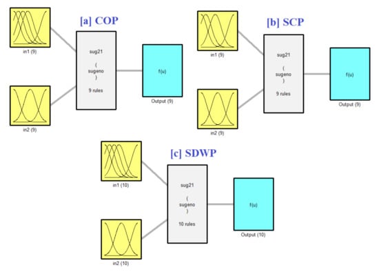
Figure 4.
Inputs and outputs of ANFIS model (a) COP; (b) SCP, and (c) SDWP.
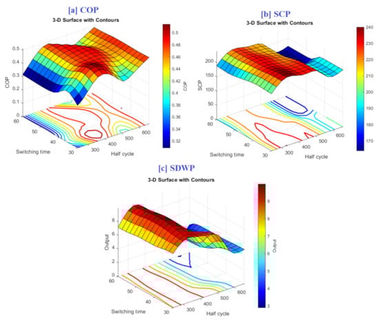
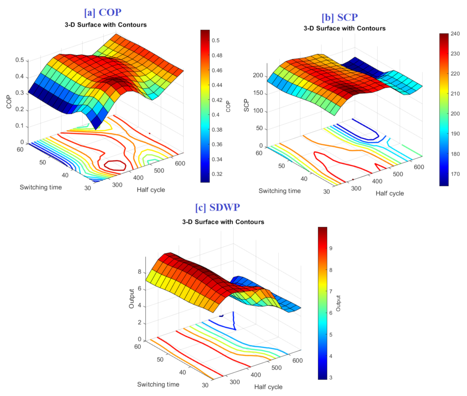
Figure 5.
3-D surface plot of output performance changing values related to input parameters (a) COP; (b) SCP, and (c) SDWP.
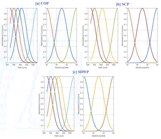
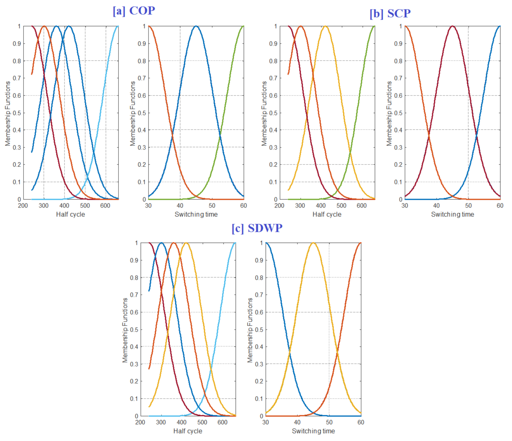
Figure 6.
Inputs membership functions of the fuzzy system (a) COP; (b) SCP, and (c) SDWP.
The main goal of this research and this technique is that we can study many cases and study the effect of changing many factors at the same time, which saves a lot of time and effort. It would be difficult to study these factors together in a laboratory, so this study explores what we can do and summarizes many practical experiments to bring us to the best-operating conditions as shown in Figure 5. The figure shows the effect of cycle time and switching time on the performance parameters of the systems which are COP, SCP, and SDWP. The COP could be reached up to 0.5 by increasing the cycle time were changing the switching time has a marginally effect on the COP. By longing the cycle time more amount of pure water is generated which raises the COP.
The effect of changing cycle time is very clear when dealing with SDWP as shown in Figure 5c. Increasing half-cycle time up to 300 s has a good impact on the SDWP however behind this limit, the SDWP shows a drop. This indicates that however, the desalinated water amount may increase by increasing cycle time, the benefits of this are dissipated because of the decrease in the number of cycles that can be performed per day with the increase in cycle time.
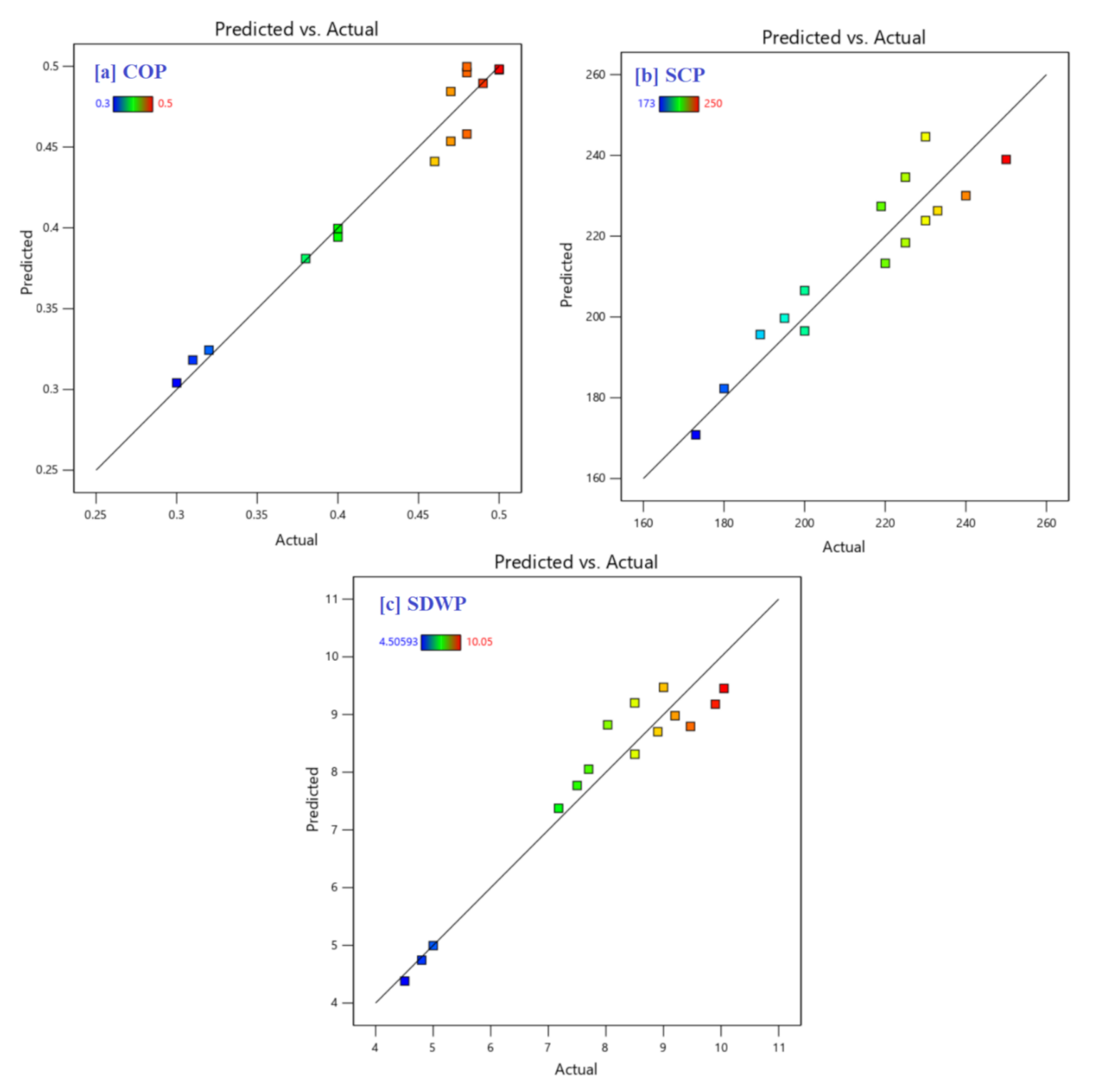
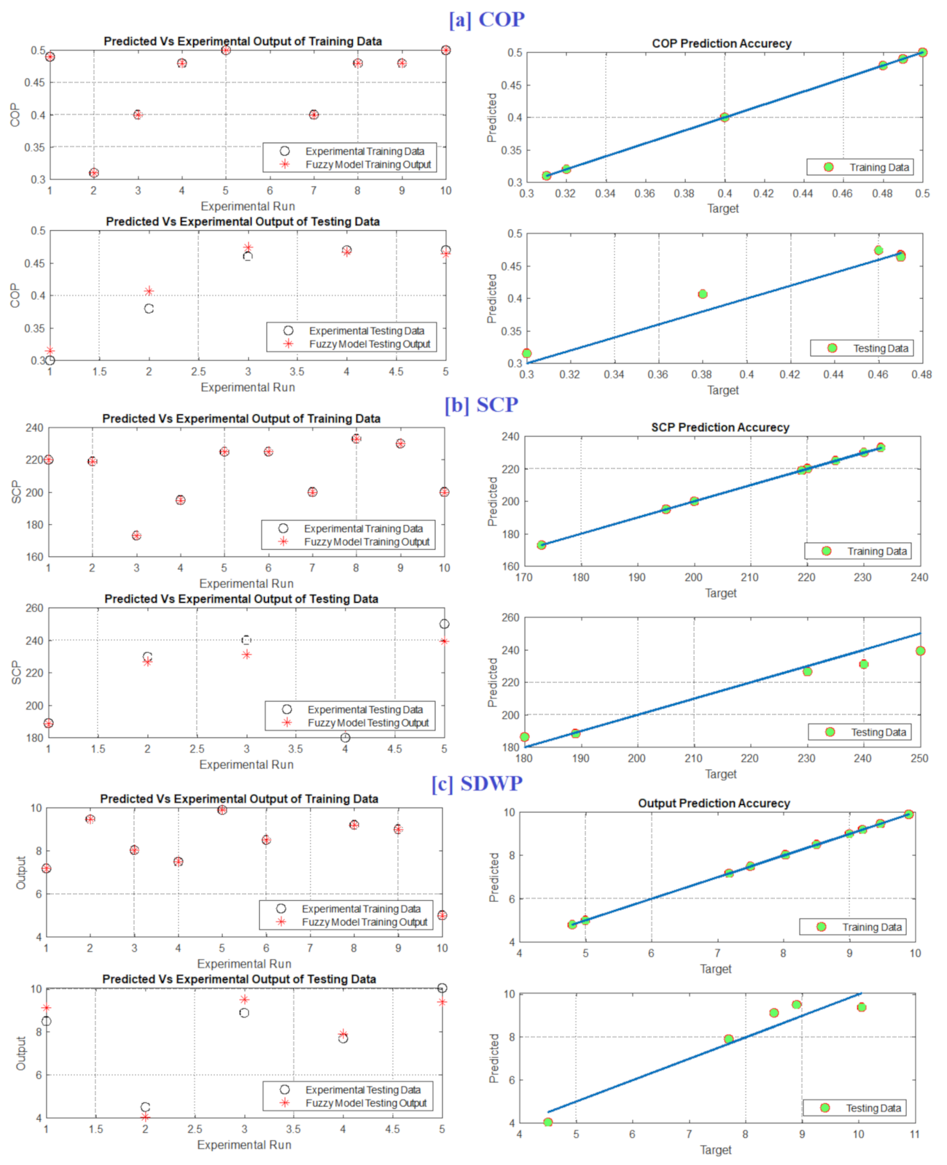
A significant measure to assess the model’s prediction precision is to plot these predictions versus their corresponding targets. Consequently, Figure 7 presents the accuracy plots of COP, SCP, and SDWP models. Considering Figure 7, it is clear that for COP, SCP, and SDWP models, the training and the testing predictions are distributed closer to the one hundred percent accuracy line that matches with the obtained high values of the R2.
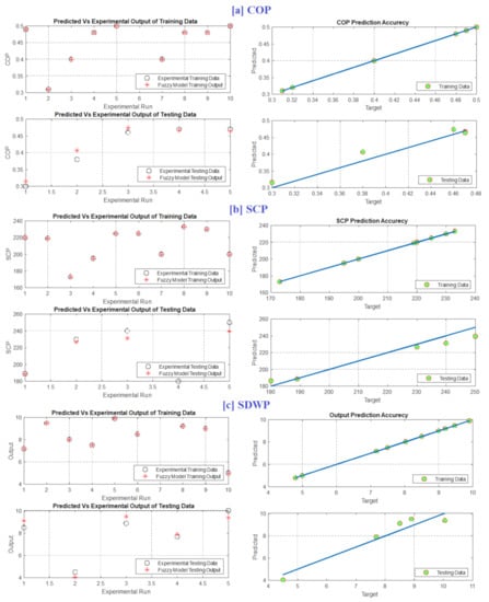
Figure 7.
Comparison of the training and testing data (a) COP; (b) SCP, and (c) SDWP.
5. Conclusions
Based on the measured data of adsorption water desalination system (AWDS), an accurate model has been created to simulate the specific daily water production (SDWP), the coefficient of performance (COP), and specific cooling power (SCP) in terms of switching and cycle time. Adaptive Network-based Fuzzy Inference System (ANFIS) is selected to do this job because it is the beneficial product of the combination between fuzzy logic and artificial neural networks. For comparison purposes, an ANOVA model was also created. Applying ANOVA, the average coefficient-of-determination values were 0.8872 and 0.8223, respectively, for training and testing. These values are increased to 1.0 and 0.9673, respectively, for training and testing thanks to ANFIS based modeling. In addition, RMSE values using ANFIS were 0.00117, 2.5201 and 1.46 respectively, for training, testing and all data. Compared with ANOVA, the average RMSE value based on all datasets is decreased from 8.607 (ANOVA) to 1.46 by using ANFIS. This means ANFIS modelling decreased the RMSE of all datasets by 83% compared with ANOVA. In sum, the main findings confirmed the superiority of ANFIS modeling of the output performance of AWDS compared with ANOVA. In future work, modern optimization algorithms will be integrated with ANFIS modeling to identify the best operating parameters AWDS.
Author Contributions
Data curation, H.A. and A.A.; Formal analysis, A.A.A.-Z. and A.A.; Funding acquisition, H.A.; Investigation, H.A., H.R. and S.F.Z.; Methodology, H.R. and A.A.; Resources, A.A.A.-Z.; Software, S.F.Z.; Supervision, H.A.; Visualization, A.A.; Writing—original draft, H.A., H.R. and A.A. All authors have read and agreed to the published version of the manuscript.
Funding
This research received funding from the Institutional Fund Projects under grant no. (IFPRC-038-135-2020) supported by the Ministry of Education and King Abdulaziz University, Deanship of Scientific Research (DSR), Jeddah, Saudi Arabia.
Institutional Review Board Statement
Not applicable.
Informed Consent Statement
Not applicable.
Data Availability Statement
No new data were created or analyzed in this study.
Acknowledgments
This research work was funded by the Institutional Fund Projects under grant no. (IFPRC-038-135-2020). Therefore, authors gratefully acknowledge technical and financial support from the Ministry of Education and King Abdulaziz University, DSR, Jeddah, Saudi Arabia.
Conflicts of Interest
The authors declare no conflict of interest.
References
- Rashid, K. Design, Economics, and Real-Time Optimization of a Solar/Natural Gas Hybrid Power Plant. Doctoral Dissertation, The University of Utah, Salt Lake City, UT, USA, 2019. [Google Scholar]
- Rashid, K.; Safdarnejad, S.M.; Powell, K.M. Dynamic simulation, control, and performance evaluation of a synergistic solar and natural gas hybrid power plant. Energy Convers. Manag. 2019, 179, 270–285. [Google Scholar] [CrossRef]
- Rezk, H.; Al-Dhaifallah, M.; Hassan, Y.B.; Ziedan, H.A. Optimization and energy management of hybrid photovoltaic-diesel-battery system to pump and desalinate water at isolated regions. IEEE Access 2020, 8, 102512–102529. [Google Scholar] [CrossRef]
- Rezk, H.; Sayed, E.T.; Al-Dhaifallah, M.; Obaid, M.; Abou Hashema, M.; Abdelkareem, M.A.; Olabi, A.G. Fuel cell as an effective energy storage in reverse osmosis desalination plant powered by photovoltaic system. Energy 2019, 175, 423–433. [Google Scholar] [CrossRef] [Green Version]
- Ng, K.C.; Thu, K.; Hideharu, Y.; Saha, B.B.; Chakraborty, A.; Al-Ghasham, T. Apparatus and Method for Improved Desalination. Patent SG 170810, 2009. [Google Scholar]
- Ma, H.; Zhang, J.; Liu, C.; Lin, X.; Sun, Y. Experimental investigation on an adsorption desalination system with heat and mass recovery between adsorber and desorber beds. Desalination 2018, 446, 42–50. [Google Scholar] [CrossRef]
- Ali, S.M.; Haider, P.; Sidhu, D.S.; Chakraborty, A. Thermally driven adsorption cooling and desalination employing multi-bed dual-evaporator system. Appl. Therm. Eng. 2016, 106, 1136–1147. [Google Scholar] [CrossRef]
- Olkis, C.; Brandani, S.; Santori, G. Cycle and performance analysis of a small-scale adsorption heat transformer for desalination and cooling applications. Chem. Eng. J. 2019, 378, 122104. [Google Scholar] [CrossRef]
- Youssef, P.; Mahmoud, S.M.; Al-Dadah, R. Numerical simulation of combined adsorption desalination and cooling cycles with integrated evaporator/condenser. Desalination 2016, 392, 14–24. [Google Scholar] [CrossRef]
- Amirfakhraei, T.Z.; Khorshidi, J. Performance improvement of adsorption desalination system by applying mass and heat recovery processes. Therm. Sci. Eng. Progress 2020, 18, 100516. [Google Scholar] [CrossRef]
- Zhang, H.; Ma, H.; Liu, S.; Wang, H.; Sun, Y.; Qi, D. Investigation on the operating characteristics of a pilot-scale adsorption desalination system. Desalination 2020, 473, 114196. [Google Scholar] [CrossRef]
- Rezk, H.; Alsaman, A.S.; Aldhaifallah, M.; Askalany, A.; Abdelkareem, M.A.; Nassef, A.M. Identifying optimal operating conditions of solar-driven silica gel based adsorption desalination cooling system via modern optimization. Sol. Energy 2019, 181, 475–489. [Google Scholar] [CrossRef]
- Tanveer, W.H.; Rezk, H.; Nassef, A.; Abdelkareem, M.A.; Kolosz, B.; Karuppasamy, K.; Aslam, J.; Gilani, S.O. Improving fuel cell performance via optimal parameters identification through fuzzy logic based-modeling and optimization. Energy 2020, 204, 117976. [Google Scholar] [CrossRef]
- Yousef, B.A.A.; Rezk, H.; Abdelkareem, M.A.; Olabi, A.G.; Nassef, A.M. Fuzzy modeling and particle swarm optimization for determining the optimal operating parameters to enhance the bio-methanol production from sugar cane bagasse. Int. J. Energy Res. 2020, 44, 8964–8973. [Google Scholar] [CrossRef]
- Stuart-Dahl, S.; Martinez-Guerra, E.; Kokabian, B.; Gude, V.G.; Smith, R.; Brooks, J. Resource recovery from low strength wastewater in a bioelectrochemical desalination process. Eng. Life Sci. 2019, 20, 54–66. [Google Scholar] [CrossRef] [PubMed]
- Sani, F.S.; Azmi, A.S.; Ali, F.; Mel, M. Interactive effect of temperature, pH and light intensity on biodesalination of seawater by synechococcus sp. PCC 7002 and on the cyanobacteria growth. J. Adv. Res. Fluid Mech. Therm. Sci. 2018, 52, 85–93. [Google Scholar]
- Khayet, M.; Cojocaru, C.; Essalhi, M. Artificial neural network modeling and response surface methodology of desalination by reverse osmosis. J. Membr. Sci. 2011, 368, 202–214. [Google Scholar] [CrossRef]
- Rahman, S.M.A.; Nassef, A.M.; Rezk, H.; Assad, M.E.H.; Hoque, E. Experimental investigations and modeling of vacuum oven process using several semi-empirical models and a fuzzy model of cocoa beans. Heat Mass Transf. 2021, 57, 175–188. [Google Scholar] [CrossRef]
- Dritsa, V.; Rigas, F.; Doulia, D.; Avramides, E.J.; Hatzianestis, I. Optimization of Culture Conditions for the Biodegradation of Lindane by the Polypore Fungus Ganoderma australe. Water Air Soil Pollut. 2009, 204, 19–27. [Google Scholar] [CrossRef]
Publisher’s Note: MDPI stays neutral with regard to jurisdictional claims in published maps and institutional affiliations. |
© 2021 by the authors. Licensee MDPI, Basel, Switzerland. This article is an open access article distributed under the terms and conditions of the Creative Commons Attribution (CC BY) license (https://creativecommons.org/licenses/by/4.0/).