Abstract
This paper is concerned with the optimal investment strategy for a defined contribution (DC) pension plan. We assumed that the financial market consists of a risk-free asset and a risky asset, where the risky asset is subject to the Ornstein–Uhlenbeck (O-U) process, and stochastic income and inflation risk were also considered in the model. We firstly derived the Hamilton–Jacobi–Bellman (HJB) equation through the stochastic control method. Secondly, under the logarithmic utility function, the closed-form solution of optimal asset allocation was obtained by using the Legendre transform method. Finally, we give several numerical examples and a financial analysis.
1. Introduction
With the increase of the elderly population, the investment problem of the current endowment insurance system is a hot issue. The basic annuity pension plan has two modes: the defined benefit (DB) and the defined contribution (DC). In the DC pension program, the risk of investment and the longevity risk of the participants are transferred from the fund manager to the DC pension plan member, which leads to more researchers’ enthusiasm to explore the DC pension plan.
Many scholars have been devoted to the study of the DC pension plan. Vigna and Haberman [1] put forward the discrete pension for the first time, and the dynamic programming method was applied to the optimal investment strategy of the DC pension plan. Thomson et al. [2] aimed to maximize the expected utility of the participant in the DC pension plan and used the continuous time stochastic dynamic programming method for the first time to obtain the optimal investment strategy before retirement. Since then, a large number of literature works have used the optimal control theory to study the DC pension plan. Devolder et al. [3] investigated the issue of the optimal investment for the DC pension plan before and after retirement. Deelstra et al. [4] studied the optimal investment strategy of the annuity pension under the condition that the terminal wealth must be greater than the minimum guarantee. Gerrard et al. [5] investigated the income drawdown option and optimal investment strategies by a stochastic optimal control problem.
Most of the research on the DC pension plan assumes that the stock price follows a geometric Brownian motion, and the expected return rate and volatility of the stock are constant or deterministic functions, which is inconsistent with reality. Some scholars have extended the model and proposed the stochastic volatility model (e.g., French et al. [6]; Pagan and Schwert [7]; Hobson and Rogers [8]). Some scholars extended the model and considered a constant variance elasticity (CEV) model. Xiao et al. [9] skillfully used the Legendre transform and duality theory to find the dominant solution of the optimal strategy of the DC pension plan. Gao et al. [10] adopted the method of stochastic control and variable separation to study the optimal investment of the DC pension plan. Zhang et al. [11] studied the optimal investment of the DC pension plan under a CEV model with a stochastic salary. Li et al. [12] considered an optimal investment problem for a defined contribution pension plan with default risk in a mean-variance framework under a CEV model. Yong et al. [13] studied the optimal investment of the DC pension plan under a CEV model. The explicit representation of the solution of the HJB equation associated with the portfolio optimization problem for an investor who seeks to maximize the expected power (CRRA) utility of the terminal wealth was derived based on the application of the Lie symmetry method to the partial differential equation.
Some earlier researchers obtained the optimal asset allocation rules without taking the effect of the inflation risk into account (e.g., Cairns et al. [14]). In fact, the inflation rate is an important statistical index in the study of macroeconomic fluctuations, and it is also the main risk that investors must face when they allocate assets. Battocchio and Menoncin [15] first introduced inflation risk to the DC pension plan and derived an optimal investment strategy. Wu and Dong [16] studied a multiperiod mean-variance-defined contribution pension plan. Three decision risks including the price risk of the financial asset, inflation risk, and salary risk were considered. Chen et al. [17] found an optimal asset allocation strategy for a loss-aversion DC pension plan member with a minimum performance constraint and inflation risk. Wang et al. [18] introduced the European call option and applied the martingale method to study the optimal investment of the DC pension under inflation and a minimum guarantee. Song and Chen [19] mainly studied the optimal investment strategy of two DC pension managers with strategy interaction under inflation risk. Different from the traditional method, they considered the more complicated situation in which pension managers focus on both relative wealth and relative risk aversion. Wang et al. [20] investigated a robust optimal portfolio choice problem for a DC pension plan member. The member has a stochastic salary, considers inflation risk, and invests his/her pension account wealth into a financial market consisting of a risk-free asset, an inflation-indexed bond, and a stock whose expected return rate follows a mean-reverting process.
In addition, some researchers have used Ornstein–Uhlenbeck (O-U) models to describe the prices of risky assets. Maenhout [21] analyzed the optimal investment strategy under ambiguity where the dynamics of the risk premium was formulated as an O-U process and provided a method to calculate detection-error probabilities. Gu et al. [22] assumed that the risky asset price meets the O-U model and studied the optimal investment problem of the DC pension plan when the pension manager’s preference is the power utility function. Guan and Liang [23] studied the optimization problem of the DC pension plan under the mean-variance criterion. The interest rate followed an affine model, and the market price of the stock index was the O-U process. The closed forms of the efficient frontier and the efficient strategies were derived.
In the geometric Brownian motion, the expected return rate is a constant; this means that there exists a force that makes the price of the stock run in the same direction all the time. Actually, this is not reasonable in practice, that is to say, it cannot describe the volatility of the expected return. In this paper, we use the O-U process instead of the standard geometric Brownian motion to describe the price of the risky asset. In real life, it is difficult for everyone’s income to be fixed. Therefore, we considered the situation of stochastic income. For long-term financial planning of the DC pension, not only financial risk, but also inflation risk must be considered. The inflation risk affects the optimal financial decision significantly. Therefore, to incorporate inflation risk into the DC pension plan, we assumed that financial market consists of a risk-free asset and a risky asset, where the risky asset is subject to the O-U process and the stochastic income is also considered in the model. The object of the problem is to maximize the expected utility. We established the mathematical foundation for the DC pension plan by using the dynamic programming principle. For the logarithmic utility case, the explicit solution to the optimal strategy was derived by the Legendre transform method. Finally, we give several numerical examples and financial analysis.
This paper is organized as follows. In Section 2, we describe the assumptions about the DC pension plan. In Section 3, we establish the mathematical model for the optimization problem by using the dynamic programming principle. In Section 4, we provide a verification theorem for the HJB equation related to the problem. In Section 5, we derive the explicit solution of the optimal investment strategy with the logarithmic utility function by using the Legendre transform method. In Section 6, we give several numerical examples to illustrate the effects of the model parameters on the optimal investment strategy. In Section 7, we conclude the paper.
2. Model Hypothesis
Suppose that the financial market consists of two financial assets: a risk-free asset and a single risky asset, and the risky asset is governed by the O-U process. Next, we describe the dynamic process of these two asset prices and the dynamic process of wealth.
2.1. Financial Market
Assume that our financial market is smooth, being free of transaction fees. What is more, let all the stochastic processes be defined on the probability space .
We denote the price of the risk-free asset (e.g., the bank account) at time t by , whose dynamics can be expressed as:
where is a constant rate of interest.
In the traditional model, we often think that the price of the risky asset is subject to geometric Brownian motion (GBM). However, the O-U process can better reflect the instantaneous interest rate on stock prices in the capital market. Therefore, we assumed that the price of risky assets in this paper is subject to the exponential O-U process. Let the price of the risky asset (e.g., the stock) at time t be , and suppose that the value of the risky asset at time t is described by the stochastic differential equation:
Here, the constants , , and represent the recovery rate, the response center, and the volatility, respectively.
2.2. Stochastic Income
Due to the labor wage directly impacting the investment, let denote the salary at time t. The dynamics of is driven by:
where is the appreciation rate, is the instantaneous volatility.
2.3. Inflation Risk
The inflation rate is prevalent in the modern economic market. It becomes the main factor affecting the time value of money. The payment of an enterprise annuity occurs overa long time, so we must consider the impact it will have on the investment income. To capture the inflation risk, we define a stochastic price level according to GBM:
where the constant is the expected rate of inflation, the constant is the volatility of the price level.
3. Model Formulation
3.1. Wealth Process
We define the retirement moment for T and assume that the contribution rate of the enterprise annuity is a constant c, and in each period, flows into the account of the enterprise annuity. Let denote the pension wealth at time , be the fraction of the wealth invested in the risky asset, and be the fraction of the wealth invested in the risk-free asset at time t. Then, the wealth process satisfies the following stochastic differential equation (SDE):
Introducing (1) and (2) in (5), we have
In this paper, we consider the impact of inflation risk on the optimal investment of the annuity, so the real wealth value can be expressed as the ratio of the wealth value to the inflation risk, namely . According to It’s formula, the wealth process of the enterprise annuity can be expressed as follows:
Let , and is given by:
3.2. The HJB Equation
From the above section, investors will retire at time T and have a poor risk tolerance. Moreover, suppose that the pension investor’s objective is to maximize the expected utility of the terminal wealth at retirement. To capture the investor’s preferences in the spirit of the von Neumann–Morgenstern expected utility theory, we introduce a strictly increasing and concave utility function . Thus, our problem of study can be formulated as follows:
where is the value function, and takes values in a control set .
The HJB equation is given by:
where .
Using the first-order condition for the maximizing problem, the optimal strategy yields:
Here,
Substituting (11) into (10), we derive:
It was difficult for us to obtain the solution to Equation (12). Then, we found that after using the dual transformation, the solution of the partial differential equation can be expressed.
4. Verification Theorem
In the above section, the HJB equation is derived by using the dynamic programming principle. Next, by the standard method used by Halil Mete Soner in [24], we provide the following verification theorem for the HJB equation related to our problem.
Theorem 1.
Let be a solution to Equation (10), where , then:
- for any initial data and control process π, where
- If for any initial data , there exists satisfying:then , where the operator is defined by:
Proof.
(1) Using It’s formula, we have:
Since H is a solution to Equation (10), we obtain:
Therefore,
According to the terminal condition, we obtain:
(2) Similarly,
Since H is a solution to Equation (10), we obtain:
Thus,
According to the terminal condition, we obtain:
□
5. Model Solution
5.1. Legendre Transform
Definition 1.
(see [25]) Let f: be a convex function; for , define the Legendre transform:
the function is called the Legendre dual of the function .
Suppose is a convex function and it takes the maximum value at , then:
so we may write:
Example 1.
Suppose that . If we strive to maximize , then . We also have:
We further utilize to define the Legendre transform:
where is the dual variable of x. The value of x where this optimum is attained is denoted by , so that:
and this leads to:
where and . The function is related to g by:
At the terminal time T, we define:
then:
In general, G is taken as the inverse of the marginal utility. We note that , so that:
Meanwhile, the boundary condition is:
Drawing on the experience of Jonsson and Sircar et al. [25] and by differentiating (15) with respect to t, s, , and z, the transformation rules for the derivatives of the value function H and the dual function can be given by:
Substituting (17) into (12), we derive the following equation:
Differentiating on both sides with respect to t, s, , and z, we have the following partial derivatives:
Therefore, differentiating (18) for with respect to z, we substitute (19) into (18) and then obtain:
Finally, (11) can be rewritten as:
5.2. The Solution under the Logarithm Utility Function
Next, we select the logarithm utility function (see Irgens and Paulsen [26]),
Under this special utility function, we can find the explicit solution.
According to and the form of the logarithm utility function, we obtain:
Theorem 2.
We now consider the logarithm utility function. The price of the risk-free asset, the price of the risky asset, the stochastic income, the inflation risk, and the wealth process satisfy (1)–(8), respectively, the expected maximum utility of the enterprise annuity for Problem (9) is given by:
and the corresponding optimal investment strategy is obtained as:
Here,
Proof.
The proof was inspired by Xiao et al. [9], and we try to fit a solution of the form:
with boundary conditions given by and . Substituting (23) into (20), we obtain:
We divide (24) into two equations and obtain the first equation:
Furthermore, the second equation is:
Taking into account the boundary condition , we can have one solution:
then we can conjecture a solution of (26) with the following structure:
where , .
Substituting (28) back into (26), we derive:
Eliminating the dependence on t and , we obtain:
According to the above two equations and the boundary condition, we obtain:
As a result,
Again, in terms of , we have:
Thus, (11) can be rewritten as:
In addition, combined (32) with , we obtain:
Integrating both sides of Equation (34), we derive:
Based on and the boundary condition , we obtain:
Furthermore, according to and , we have:
□
6. Numerical Analysis
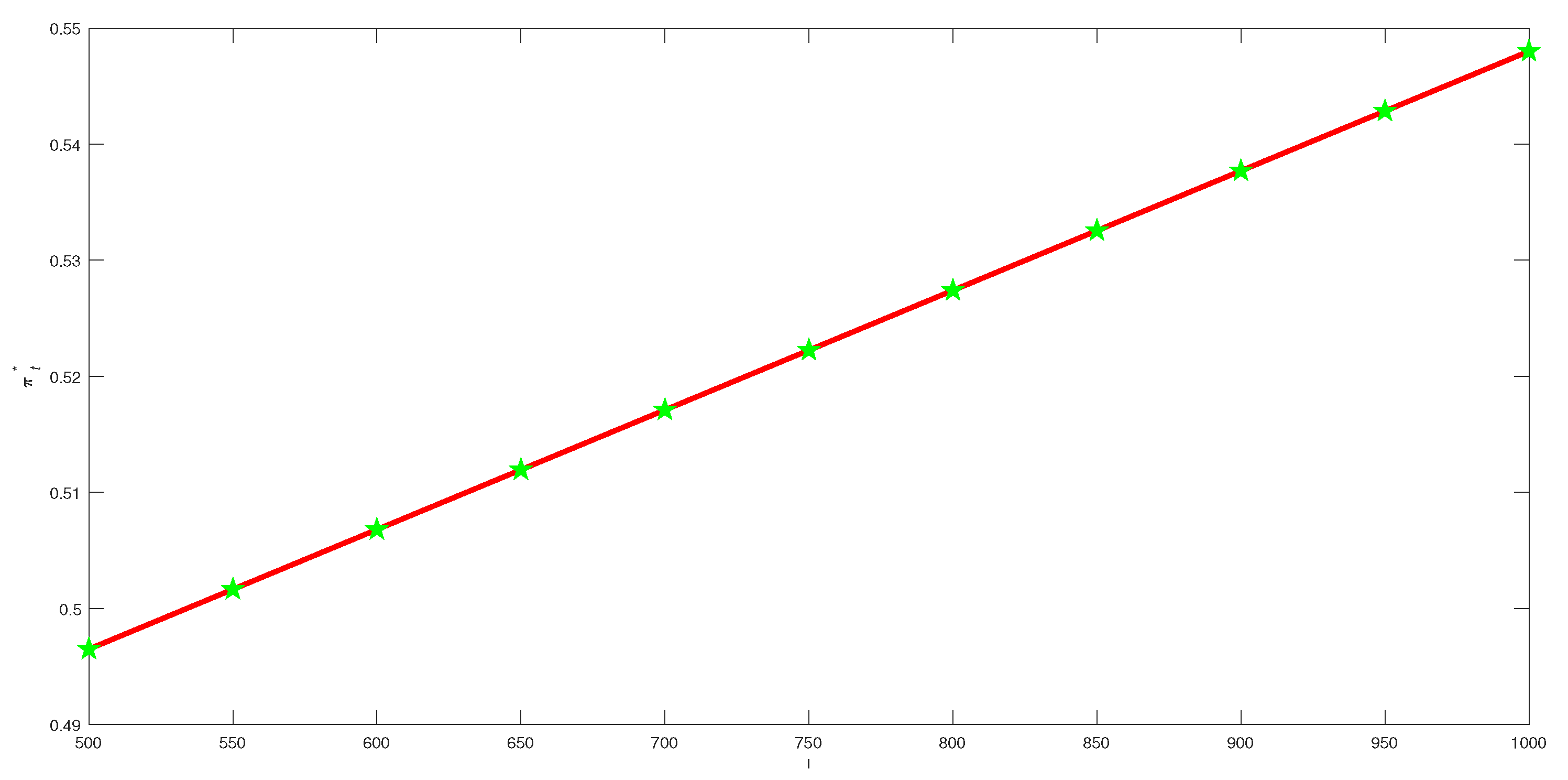
In the above section, by using the Legendre transform method under the inflation risk, we obtain the optimal investment strategy of the enterprise annuity. In order to further verify the effectiveness of its optimal investment strategy in financial market, we used the MATLAB software to analyze the influence of each parameter on the investment strategy. The basic model parameters are given by , , , , , .
In Figure 1, when the employee salary level l increases, the optimal investment on the risky asset decreases. Its financial significance is that the higher the employee’s income is, the better the living reserve fund and the stronger the risk tolerance are, so that the investment behavior is more aggressive. In order to achieve a higher yield, the annuity manager will take more capital to purchase the risky asset product.
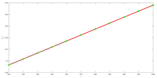
Figure 1.
Effects of parameter l on .
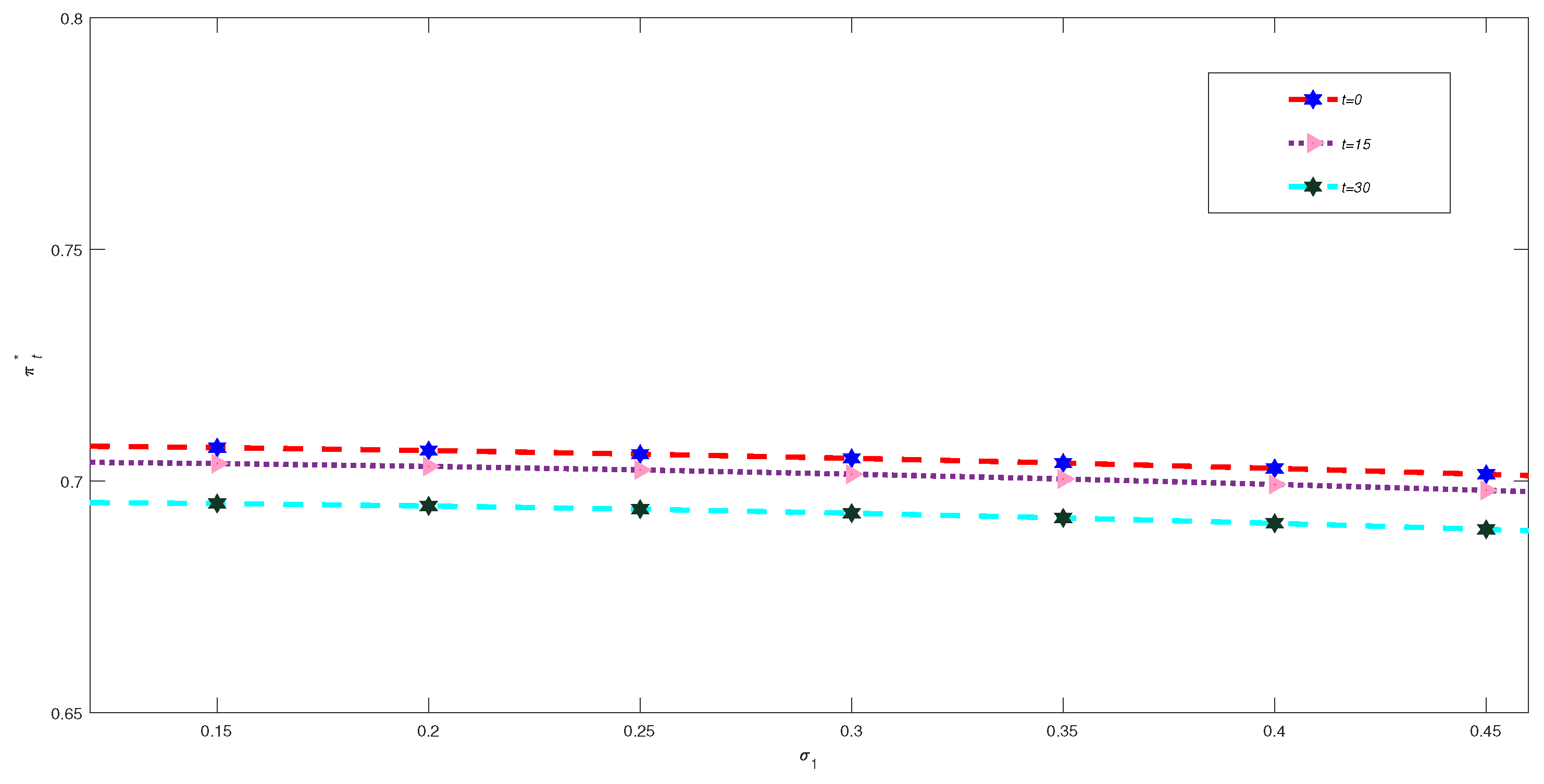
Figure 2 shows that the effect of on the optimal investment strategy is negative. The optimal strategy of the investment in risky assets with the employee’s wage decreases with the increasing of the level of volatility. Since the employee’s salary income is not stable and the risk resistance is weak, the administrator will adopt a conservative investment behavior in order to increase the guarantee, that is the funds will be more likely to flow into a risk-free asset product of a healthy income class. In addition, under certain conditions of wage level volatility, the working time is longer, and the ratio of investment to risky assets will gradually decrease. Because the employee’s income has been reduced significantly compared to before retirement, the risk appetite is also reduced. In the process of investment activities, it is necessary to avoid high risk and diversification, and the managers should first consider investment safety and risk prevention, which is mainly based on prudent returns. They are more willing to increase the proportion of investment in risk-free assets.
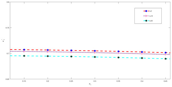
Figure 2.
Effect of parameter on .
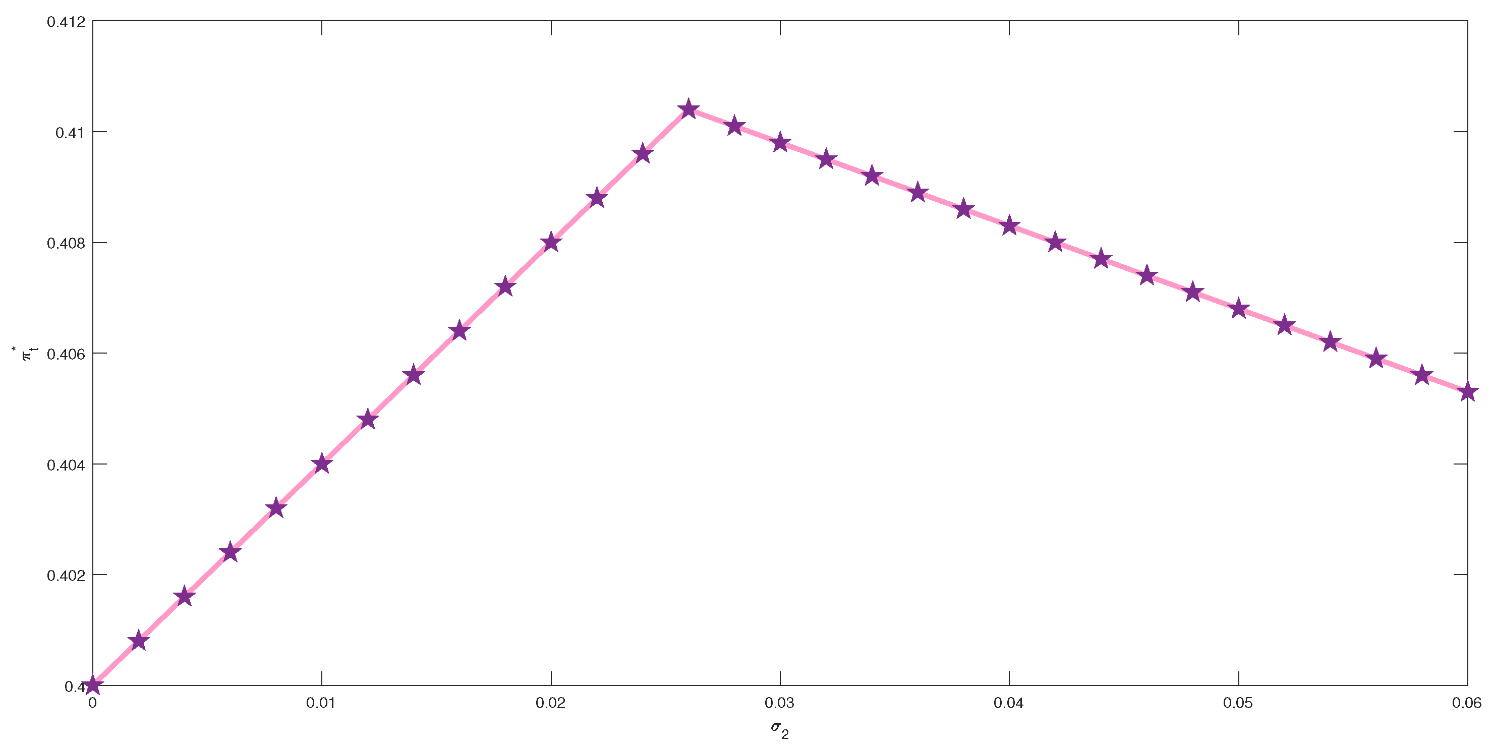
As can be seen from Figure 3, when the volatility coefficient of inflation increases, the proportion of investment in risky asset will grow. Its financial significance is that, initially, risky assets have the role of hedge inflation, and a pension manager tends to place funds on risky assets. When it is over a certain limit, the hedging will fail, such that the manager’s investment behavior is conservative and reduces the investment in risky assets, which is consistent with the actual market conditions.

Figure 3.
Effect of parameter on .
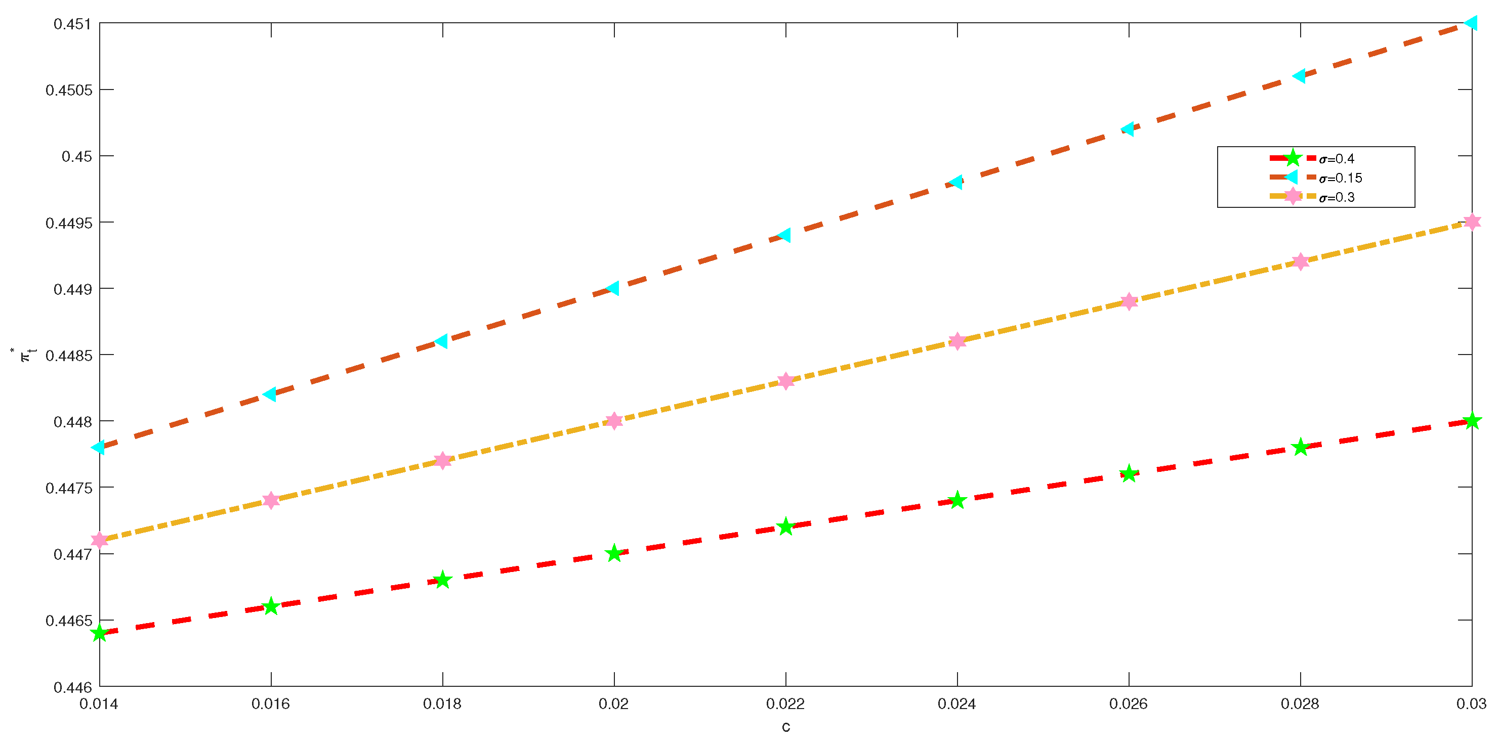
Figure 4 illustrates that the optimal proportion of investment in risky assets is positively correlated with the rate of annuity pension payment c. It shows that c decreases along with the optimal strategy . This is because an annuity pension can be obtained to improve the quality of life after retirement, especially the quality of life of well-paid personnel. The contribution rate of gold is higher, so investor’s retirement can receive a sufficient guarantee. At the same time, under the same conditions, the higher the payment rate, the more secure the investor’s life will be when he/she retires. Because of the high volatility of the stock market, the financial market becomes more unstable. When it comes to risks and benefits, security is generally considered before profitability, and the annuity pension investors will be more inclined to inject funds into the risk-free assets.
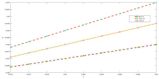
Figure 4.
Effect of parameter c on .
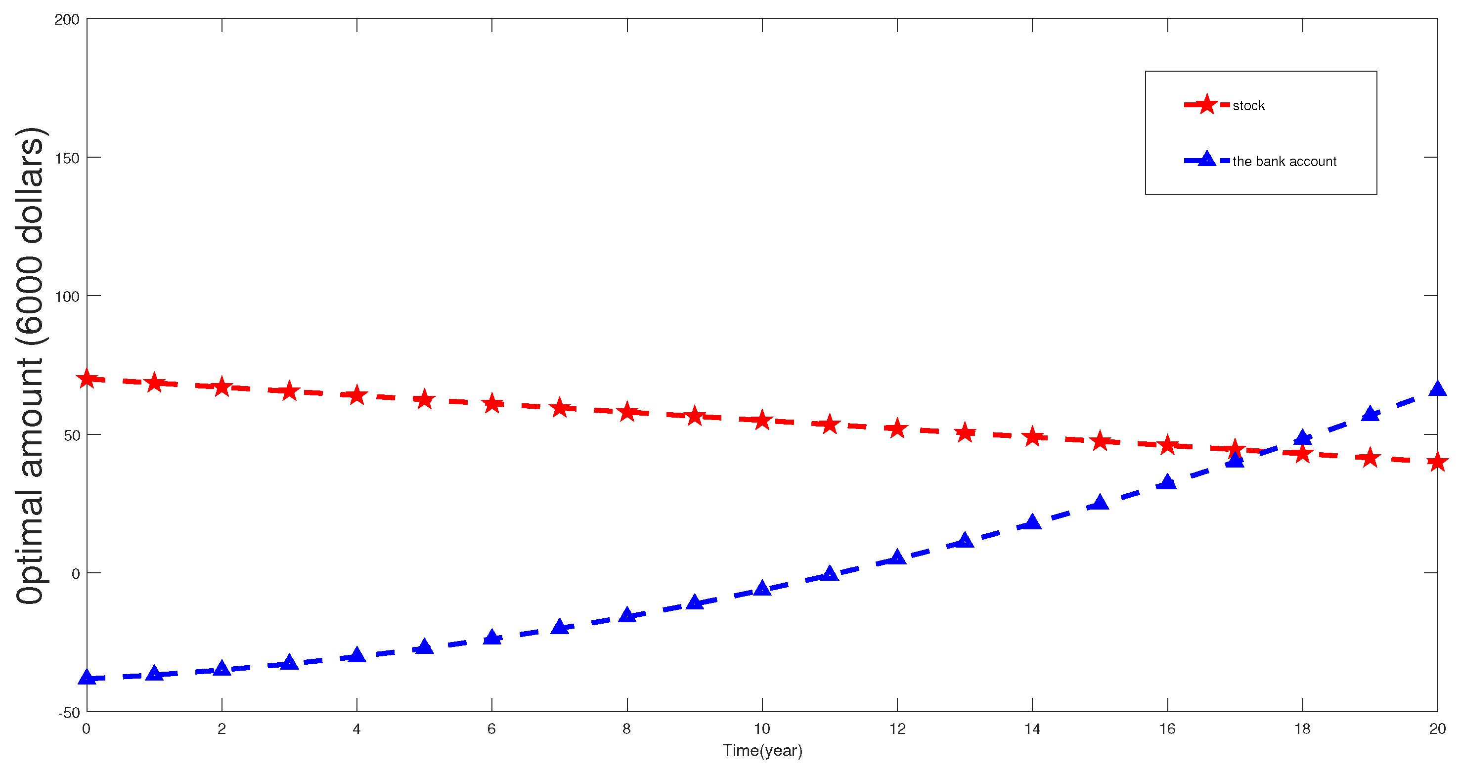
In the modern economic market, inflation is a common phenomenon and has a great influence on investment. Comparing Figure 5 with Figure 6, it can be observed that in the event of inflation in the market, the price level will rise and the purchasing power will decline. Investors are inclined to invest more in stocks and risk-free assets.
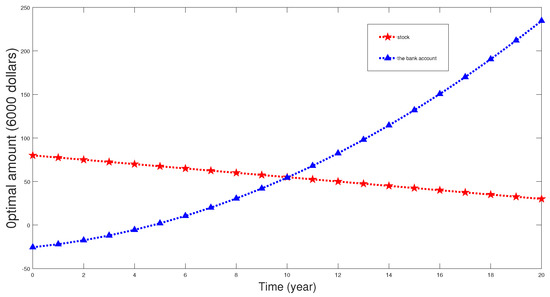
Figure 5.
Optimal amount with inflation.

Figure 6.
Optimal amount without inflation.
7. Conclusions
In this paper, the HJB equation was established for optimal dynamic asset allocation with the random income and inflation under the Ornstein–Uhlenbeck model, so as to maximize the goal of the expected effectiveness. By means of the mathematical method of the Legendre transform and separation variables, the HJB equation was reduced in dimension to obtain the explicit solution of the optimal investment strategy for the DC pension plan. Then, we analyzed the parameters of the optimal investment strategy. Some conclusions are as follows. The wage is positively correlated with the optimal strategy, while the wage volatility is negatively correlated. There will be a turning point for the impact of the inflation volatility coefficient. At the beginning, the proportion of investment in risky assets will increase with its increase, but it will decrease when it crosses the turning point. The contribution rate of the enterprise annuity also promotes the optimal proportion of investment in risky assets. Our research can provide some theoretical and practical help to annuity pension managers.
Author Contributions
Writing—review and editing, funding acquisition, and methodology, Y.W.; writing—original draft, X.X.; supervision, J.Z. All authors read and agreed to the published version of the manuscript.
Funding
This work was supported in part by the National Natural Science Foundation for Young Scientists of China (No. 11701377) and the MOE (Ministry of Education in China) Project of Humanities and Social Sciences (No. 18YJAZH127) and Shanghai Soft Science Key Foundation “Science-Technology Innovation Action” (No. 21692108000).
Institutional Review Board Statement
Not applicable.
Informed Consent Statement
Not applicable.
Data Availability Statement
Not applicable.
Acknowledgments
The authors would like to thank the reviewers for their very helpful comments and suggestions.
Conflicts of Interest
The authors declare no conflict of interest.
References
- Vigna, E.; Haberman, S. Optimal investment strategy for defined contribution pension schemes. Insur. Math. Econ. 2001, 28, 233–262. [Google Scholar] [CrossRef]
- Thomson, R.J. The use of utility functions for investment channel choice in defined contribution retirement fund, I: Defence. Br. Actuar. J. 2003, 9, 653–709. [Google Scholar] [CrossRef]
- Devolder, P.; Princep, M.B.; Fabian, I.D. Stochastic optimal control of annuity contracts. Insur. Math. Econ. 2003, 33, 227–238. [Google Scholar] [CrossRef]
- Deelstra, G.; Grasselli, M.; Koehl, P.F. Optimal investment strategies in the presence of a minimum guarantee. Insur. Math. Econ. 2003, 33, 189–207. [Google Scholar] [CrossRef] [Green Version]
- Gerrard, R.; Haberman, S.; Vigna, E. Optimal investment choices post-retirement in a defined contribution pension scheme. Insur. Math. Econ. 2004, 35, 321–342. [Google Scholar] [CrossRef] [Green Version]
- French, K.R.; Schwert, G.W.; Stambaugh, R.F. Expected stock returns and volatility. J. Financ. Econ. 1987, 19, 3–29. [Google Scholar] [CrossRef] [Green Version]
- Pagan, A.R.; Schwert, G.W. Alternative models for conditional stock volatility. J. Econom. 1990, 45, 267–290. [Google Scholar] [CrossRef] [Green Version]
- Hobson, D.G.; Rogers, L.C.G. Complete models with stochastic volatility. Math. Financ. 1998, 8, 27–48. [Google Scholar] [CrossRef]
- Xiao, J.W.; Zhai, H.; Qin, C.L. The constant elasticity of variance (CEV) model and the legendre transform-dual solution for annuity constracts. Insur. Math. Econ. 2006, 40, 302–310. [Google Scholar] [CrossRef]
- Gao, J.W. Optimal portfolios for DC pension plans under a CEV mode. Insur. Math. Econ. 2009, 44, 479–490. [Google Scholar] [CrossRef]
- Zhang, C.B.; Rong, X.M.; Chang, H. Optimal Investment for DC Pension with stochastic salary under a CEV model. Chin. J. Eng. Math. 2013, 30, 1–9. [Google Scholar]
- Li, D.; Rong, X.; Zhao, H.; Yi, B. Equilibrium investment strategy for DC pension plan with default risk and return of premiums clauses under CEV model. Insur. Math. Econ. 2017, 72, 6–20. [Google Scholar] [CrossRef]
- Yong, X.; Sun, X.; Gao, J. Symmetry-based optimal portfolio for a DC pension plan under a CEV model with power utility. Nonlinear Dyn. 2021, 103, 1775–1783. [Google Scholar] [CrossRef]
- Cairns, A.J.; Blake, D.; Dowd, K. Stochastic lifestyling: Optimal dynamic asset allocation for defined contribution pension plans. J. Econ. Dyn. Control 2005, 30, 843–877. [Google Scholar] [CrossRef] [Green Version]
- Battocchio, P.; Menoncin, F. Optimal pension management in a stochastic framework. Insur. Math. Econ. 2004, 34, 79–95. [Google Scholar] [CrossRef]
- Wu, H.L.; Dong, H.B. Multi-period mean-variance defined contribution pension management with inflation and stochastic income. Syst. Eng. Theory Pract. 2016, 36, 545–558. [Google Scholar]
- Chen, Z.; Li, Z.F.; Zeng, Y. Asset allocation under loss aversion and minimum performance constraint in a DC pension plan with inflation risk. Insur. Math. Econ. 2017, 75, 137–150. [Google Scholar] [CrossRef]
- Wang, C.Y.; Fu, C.Y.; Sheng, G.X. Optimal investment of DC Pension under the inflation and minimum guarantee. Oper. Res. Manag. Sci. 2018, 27, 193–199. [Google Scholar]
- Song, A.; Chen, P. Relative performance concern on DC pension plan under Heston model with inflation risk. Math. Probl. Eng. 2020, 2020, 5180286. [Google Scholar]
- Wang, P.; Li, Z.; Sun, J. Robust portfolio choice for a DC pension plan with inflation risk and mean-reverting risk premium under ambiguity. Optimization 2021, 70, 191–224. [Google Scholar] [CrossRef]
- Maenhout, P.J. Robust portfolio rules and detection-error probabilities for a mean-reverting risk premium. J. Econ. Theory 2006, 128, 136–163. [Google Scholar] [CrossRef]
- Gu, A.; Li, Z.; Zeng, Y. Optimal investment strategy under Ornstein–Uhlenbeck mode for a DC pension plan. Acta Math. Appl. Sin. 2013, 36, 715–726. [Google Scholar]
- Guan, G.; Liang, Z. Mean-variance efficiency of the DC pension plan under stochastic interest rate and mean-reverting returns. Insur. Math. Econ. 2015, 61, 99–109. [Google Scholar] [CrossRef]
- Soner, H.M. Controlled Markov processes, viscosity solutions and applications to mathematical finance. In Viscosity Solutions and Applications; Dolcetta, I.C., Lions, P.L., Eds.; Springer: Berlin, Germany, 1997; Volume 1660, pp. 134–185. [Google Scholar]
- Jonsson, M.; Sircar, R. Optimal investment problems and volatility homogenization approximations. In Modern Methods in Scientific Computing and Applications; Bourlioux, A., Gander, M.l., Eds.; Springer: Dordrecht, The Netherlands, 2002; pp. 255–281. [Google Scholar]
- Irgens, C.; Paulsen, J. Optimal control of risk exposure, reinsurance and investments for insurance portfolios. Insur. Math. Econ. 2004, 35, 21–51. [Google Scholar] [CrossRef]

Publisher’s Note: MDPI stays neutral with regard to jurisdictional claims in published maps and institutional affiliations. |
© 2021 by the authors. Licensee MDPI, Basel, Switzerland. This article is an open access article distributed under the terms and conditions of the Creative Commons Attribution (CC BY) license (https://creativecommons.org/licenses/by/4.0/).