Article

Node Generation for RBF-FD Methods by QR Factorization

1
Department of Mathematics and Statistics, Air Force Institute of Technology, Dayton, OH 45433, USA
2
School of Mathematical and Statistical Sciences, Arizona State University, Tempe, AZ 85281, USA
*
Author to whom correspondence should be addressed.
Mathematics 2021, 9(16), 1845; https://doi.org/10.3390/math9161845
Submission received: 29 June 2021 / Revised: 29 July 2021 / Accepted: 30 July 2021 / Published: 5 August 2021
(This article belongs to the Special Issue Applied Mathematics and Computational Physics)

Abstract

:
Polyharmonic spline (PHS) radial basis functions (RBFs) have been used in conjunction with polynomials to create RBF finite-difference (RBF-FD) methods. In 2D, these methods are usually implemented with Cartesian nodes, hexagonal nodes, or most commonly, quasi-uniformly distributed nodes generated through fast algorithms. We explore novel strategies for computing the placement of sampling points for RBF-FD methods in both 1D and 2D while investigating the benefits of using these points. The optimality of sampling points is determined by a novel piecewise-defined Lebesgue constant. Points are then sampled by modifying a simple, robust, column-pivoting QR algorithm previously implemented to find sets of near-optimal sampling points for polynomial approximation. Using the newly computed sampling points for these methods preserves accuracy while reducing computational costs by mitigating stencil size restrictions for RBF-FD methods. The novel algorithm can also be used to select boundary points to be used in conjunction with fast algorithms that provide quasi-uniformly distributed nodes.

1. Introduction

In [1,2,3,4,5,6], Polyharmonic Splines (PHSs) and polynomials were combined to generate radial basis function finite-difference (RBF-FD) methods. One of the key benefits of combining PHSs with polynomials was the fact that high-order accuracy could be obtained from resulting RBF-FD differentiation matrices. Another improvement was the elimination of the requirement to select optimal shape parameters. When implementing RBF-FD methods, the choice of shape parameter plays a crucial role in the conditioning of interpolation matrices as well as accuracy [7,8]. As a result, the need to balance accuracy and conditioning through the tuning of the shape parameter becomes a problem itself. The use of PHSs with polynomials eliminates this requirement. Instead of having to select shape parameters to handle different resolutions, the only parameter selection required is the degree of the PHS and polynomials used, which is pre-selected and remains constant.
The need to tune the shape parameter can be observed in the stagnation error of RBF-FD methods strictly using RBFs. These methods encountered convergence, which plateaued or worsened as the number of sampling points increased. This was directly due to the fact that as the resolution increases, the shape parameter needed to be tuned. As a result, accuracy was traded off in order to maintain the conditioning of interpolation matrices. The implementation of RBF-FD matrices using PHSs and polynomials eliminated such stagnation error. These methods maintain accurate approximations while also eliminating the complexities of shape parameter selection.
Along with these advantages for using PHSs with polynomials came one key constraint: the number of nodes used in each stencil was required to be approximately twice the size of the number of polynomial basis functions appended. For example, in [1,2], stencils comprising of 37 nodes were used. In this case, only polynomials up to degree 4 could be appended to the RBFs. The accuracy of the resulting approximation depends on the degree of the polynomials appended. Thus, for higher-order methods, larger stencils are required. This results in increased computational costs as the differentiation matrices used became less sparse since derivative calculations at each node require function values from an increased number of nearest neighbors. The stencil size then becomes a limiting factor when attempting to achieve a given order of accuracy efficiently.
RBF-FD methods using PHSs and polynomials are usually implemented using Cartesian points, hexagonal points, or quasi-uniformly distributed points. A few references that looked into the placement of sampling points for finite-difference methods include [9,10,11,12,13]; however, for RBF-FD methods in 2D, the general strategy has been to generate a set of quasi-uniformly distributed nodes based on repel algorithms in order to achieve a set spacing. The algorithms for computing these scattered nodes can be found in [14,15,16]. The points in [14,15] are generated using a spatial density function to inform the spacing of the nodes throughout the domain. Similarly, the points in [16] are generated in order to achieve a predetermined average separation between points. In this paper, we consider finding the placement of sampling points for RBF-FD methods using PHSs and polynomials by minimizing a piecewise-defined Lebesgue constant. This will be accomplished by modifying a column-pivoting QR algorithm previously used to find near-optimal sampling points for polynomial interpolation, also known as the approximate-Fekete points.
The modified column-pivoting QR algorithm presented in this work provides a novel sampling method for RBF-FD methods with three major benefits. First, the sampled points mitigate a key computational constraint of RBF-FD methods implemented with PHSs and polynomials. That is, it dramatically reduces the number of nodes per stencil for high-order approximation as compared to other node distributions such as Cartesian or hexagonal points. This reduces the computational requirements of the RBF-FD method while retaining high-order accuracy as it has been shown that the accuracy of these methods depends on the polynomial degree and not the number of nodes in each stencil [6]. The newly sampled points provide sparser differentiation matrices. The second benefit of the modified column-pivoting QR algorithm is the ability to compute sampling points with a simple, robust method. The implementation of the algorithm only requires a set of candidate points and a choice of basis. The basis used in the novel method is chosen to match the basis used for the RBF-FD computations. Thus, once a set of candidate points is chosen and input into the algorithm, a set of sampling points is provided. This provides a simple algorithm for point selection with few variable parameters. Lastly, the algorithm can be used to inform the placement of boundary points for complex 2D regions. These boundary points can then be used in conjunction with scattered repel point algorithms, which provide quasi-uniformly distributed interior points.
We introduce the basics for RBF-FD methods in Section 2. In Section 3, we introduce the novel piecewise-defined Lebesgue constant used to compare sampling point locations for local RBF-FD methods. In this section, we also introduce the modified column-pivoting QR algorithm used to generate sampling point locations for RBF-FD methods. In Section 4, we investigate the behavior of varying sampling point locations in 1D. Section 5 extends the results from 1D into 2D. Lastly, Section 6 implements test cases using the newly generated points.

2. Background

2.1. RBF Setup

A thorough introduction to RBFs methods can be found in [17,18,19,20]. The RBF interpolant is a linear combination of translates of a radially-symmetric function denoted by ϕ x x j . In 1D, interpolating through the points x j , y j gives us the interpolant of the form
s x = j = 0 n c j ϕ x x j ,
where the coefficients c k are found by solving the linear interpolation system:
ϕ x 0 x 0 ϕ x 0 x 1 ϕ x 0 x n ϕ x 1 x 0 ϕ x 1 x 1 ϕ x 1 x n ϕ x 2 x 0 ϕ x 2 x 1 ϕ x 2 x n ϕ x n x 0 ϕ x n x 1 ϕ x n x n c 0 c 1 c 2 c n = y 0 y 1 y 2 y n .
Common examples of RBFs are listed in Table 1. Most of these examples, the multiquadric, the inverse multiquadric, and the Gaussian RBFs in particular, contain the presence of the shape parameter, ε . These shape parameters must be tuned in order to balance conditioning and accuracy, and in the case where the number of sampling nodes used becomes large enough, the accuracy stagnates or decreases due to the need to condition the interpolation matrices (alternative options to shape parameter tuning are presented in [20] but are not considered in this study).
Using PHSs and polynomials, we can write the approximation as
s x = j = 0 n c j | x x j | 2 m 1 + j = 0 l c j + n + 1 x j .
See [20] for more details on RBF approximations with appended polynomials. To implement a 2D finite-difference method with RBFs, the nearest neighbors are to be used in the finite-difference weight calculations. This is accomplished using MATLAB’s KDTree and knnsearch functions. To calculate the RBF-FD weights at a given point, a stencil size is chosen and the nearest neighbors are found. These nearest neighbors are the points used in the RBF-FD calculation for the given point. Figure 1 below illustrates two examples of what these stencils should look like in a complex 2D region, such as the bumped-disk shape. The sampling points are marked by the dots, while the center point is marked by an asterisk with the relevant stencil points being outlined by circles.

2.2. Calculating RBF-FD Weights

To find the RBF-FD weights for a given operator L , we first consider the system with strictly RBFs, as shown in Equation (4).
x 0 x 0 2 2 m 1 x 0 x k 2 2 m 1 x n x 0 2 2 m 1 x n x k 2 2 m 1 w 0 w k = L x x 0 2 2 m 1 | x = x c L x x k 2 2 m 1 | x = x c .
Appending the polynomial terms, as in Equation (3), expands the linear system, as shown in Equations (5) and (6). This calculates the differentiation weights, w 0 , , w k , for the point x = x c using an k + 1 point stencil with RBFs being appended with the polynomials 1 , x , y . Thus, the top-left sub-matrix is the usual RBF interpolation matrix. We see that a Vandermonde matrix consisting of the same stencil points, but using a monomial basis, is appended to the RBF interpolation matrix. For illustration, the PHSs in this case are combined with polynomials up to the first degree; in most cases, polynomials of higher degree are appended. Here, solving for the weights gives us an RBF-FD approximation for the differentiation operator, L, using PHSs with polynomials.
V w = L ,
x 0 x 0 2 2 m 1 x 0 x k 2 2 m 1 1 x 0 y 0 x n x 0 2 2 m 1 x n x k 2 2 m 1 1 x k y k 1 1 0 0 0 x 0 x k 0 0 0 y 0 y k 0 0 0 w 0 w k w k + 1 w k + 2 w k + 3 = L x x 0 2 2 m 1 | x = x c L x x k 2 2 m 1 | x = x c L 1 | x = x c L x | x = x c L y | x = x c .
As previously mentioned, the system in Equation (5) does not contain any shape parameters, thus eliminating the need to find the optimal value for such a parameter. Instead, the conditioning of the matrix in the left-hand side is achieved by appending the polynomials while using an appropriate stencil size.

2.3. Accuracy Considerations

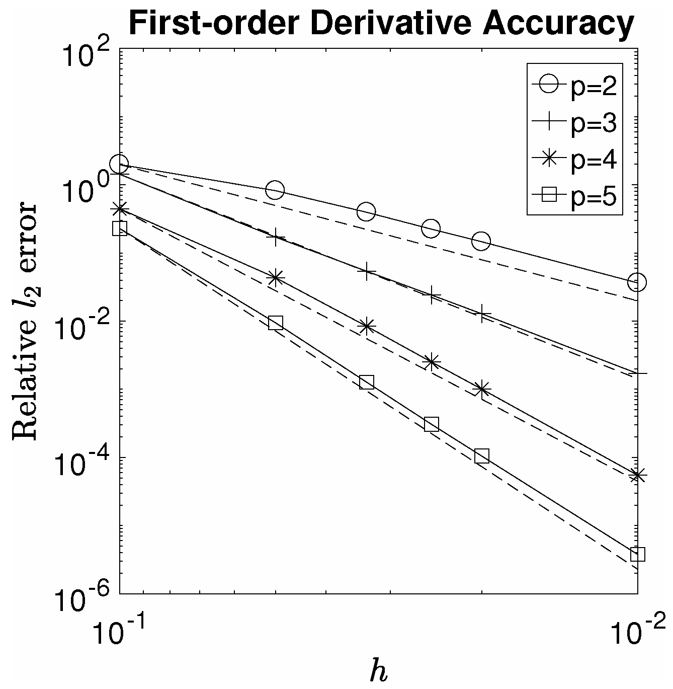
The convergence rate of RBF-FD methods combining PHSs and polynomials depends on the degree of polynomials used and is independent of both the parameter, m, which defines the PHS, and the stencil size. Thus, approximations converge at the rate of O h p , where h is the spacing and p is the degree of polynomials appended. Figure 2 below depicts an example of the convergence rate these RBF-FD methods provide. In this case, a hexagonal nodal set is used on the unit square. A 51 point stencil is used such that there are enough nodes in the stencil to handle the inclusion of polynomials up to degree p = 5 . The PHS used is ϕ r = r 3 . The relative error of the approximation of d d x 1 + sin 4 x + cos 3 x + sin 2 y is plotted against the spacing, h, along with the expected convergence rate for each degree of polynomials used in dashed lines.

3. Node Sampling for RBF-FD Methods

To find sampling points for RBF-FD methods, we calculate the set of points with a minimal Lebesgue constant. Lebesgue constants are commonly used to determine the optimality of sets of sampling points for polynomial interpolation. The goal will be to formulate a piecewise-defined Lebegue constant for RBF-FD methods. Previous works [9,10,11,12] have looked to find point locations for finite-difference methods but do not formulate piecewise-defined Lebesgue constants and have not focused on RBF-FD methods using PHSs and polynomials. A few works, however, have considered Lebesgue constants for RBF-FD methods for other purposes [21,22].

3.1. The Piecewise-Defined Lebesgue Constant for RBF-FD Methods

To formulate a notion of the Lebesgue constant for RBF-FD methods, we first recall that for polynomial interpolation, given a set of n + 1 sampling points, x 0 , y 0 , , x n , y n , the Lebesgue constant is defined as:
Λ = sup f p f f = sup x , y j = 0 n | l j x , y | .
Here, p is the approximation of functions f C 1 , 1 and the l j ’s are the cardinal functions which satisfy:
l j x k , y k = 1 k = j 0 k j .
To define the Lebesgue constant for RBF-FD methods, the cardinal functions must be formulated similarly. Furthermore, the cardinal functions must be considered in a piecewise manner to account for the local nature of RBF-FD methods. This is accomplished by considering the piecewise cardinal functions.
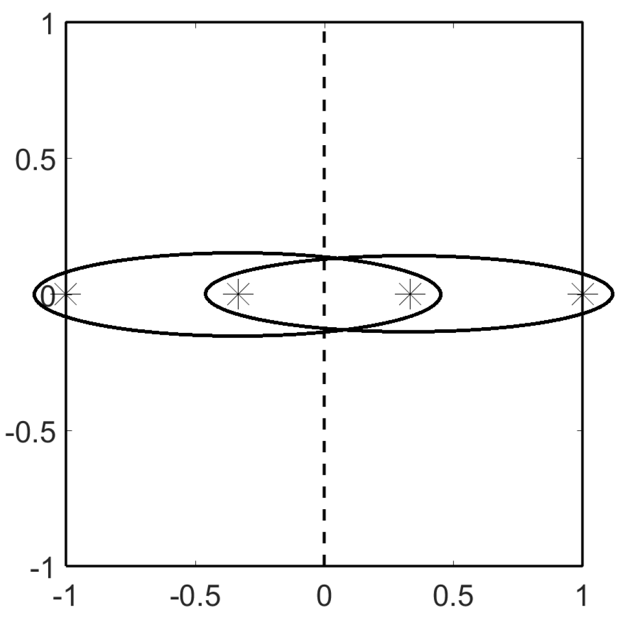
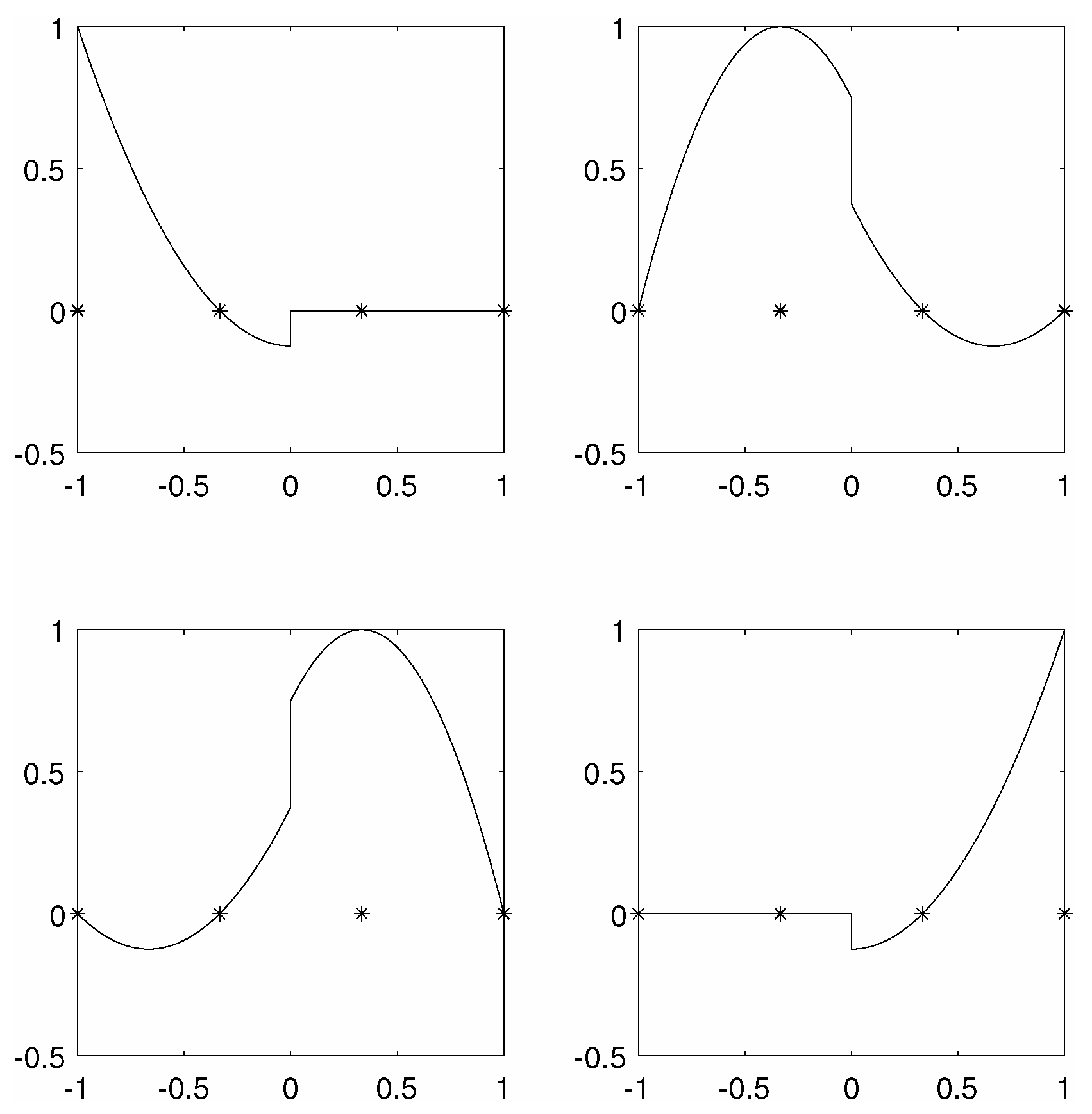
Consider 1D piecewise polynomial interpolation with 4 sampling points, 1 , 1 3 , 1 3 , 1 , using a 3 point stencil. In this case, there are two stencil groupings as outlined in Figure 3 below. For this example, the piecewise cardinal functions are shown in Figure 4. Each piecewise cardinal function contains a discontinuity at x = 0 . For a given x, each piecewise cardinal function, l j x , is defined using the 3 closest sampling points. Thus, for x 1 , 0 , the piecewise cardinal functions are defined using points 1 , 1 3 , 1 3 , while for x 0 , 1 , the piecewise cardinal functions are defined using points 1 3 , 1 3 , 1 .
For RBF-FD methods, the piecewise cardinal functions are defined similarly. Consider using a k-point stencil with degree p = 1 polynomials being appended. The given 2D region is discretized into a fine mesh, Ω , to calculate the piecewise cardinal functions on. Then, the k nearest neighbors from a given set of sampling points, x 0 , y 0 , , x n , y n , are found for each point in Ω . The cardinal function coefficients for a given stencil grouping, x 0 , y 0 , , x k , y k , can be calculated by solving the following system in Equation (9).
x 0 x 0 2 2 m 1 x 0 x k 2 2 m 1 1 x 0 y 0 x k x 0 2 2 m 1 x k x k 2 2 m 1 1 x k y k 1 1 0 0 0 x 0 x k 0 0 0 y 0 y k 0 0 0 c 0 , 0 c 0 , k c k , 0 c k , k c k + 1 , 0 c k + 1 , k c k + 2 , 0 c k + 2 , k c k + 3 , 0 c k + 3 , k = I 0 .
Once the piecewise cardinal function coefficients, C = c i , j for i = 0 , , k , j = 0 , , k , are obtained, the matrix of piecewise cardinal functions is built according to Equation (10). Here, xx 0 xx m Ω denote the points in the fine mesh that have x 0 , y 0 , , x k , y k as the k-nearest neighbors, and the indices i 0 i k are such that x 0 = x i 0 x k = x i k . Once this process is repeated for all possible stencil groupings, the full matrix of piecewise cardinal functions will have been tabulated, and the Lebesgue constant for RBF-FD methods is defined as Λ R B F F D = sup x , y j = 0 n | l j x , y | .
l = l i 0 xx 0 l i k xx 0 l i 0 xx m l i k xx m , l = xx 0 x 0 2 2 m 1 xx 0 x k 2 2 m 1 1 x x 0 y y 0 xx m x 0 2 2 m 1 xx m x k 2 2 m 1 1 x x m y y m C .

3.2. Modified Column-Pivoting QR Algorithm (MCpQR Algorithm)

In the previous section, we discussed the metric used to determine the optimality of a set of sampling points for RBF-FD methods using PHSs and polynomials. In this section, we discuss how to sample point locations using this optimality measure. The algorithm proposed is a modification of an algorithm commonly used to find near-optimal sampling points for polynomial interpolation.
Finding optimal and near-optimal sampling points for polynomial interpolation has been studied extensively [23,24,25,26,27,28,29,30,31,32,33]. A robust algorithm for near-optimal polynomial interpolation sampling is modified to be used for RBF-FD methods. This method, which performs column-pivoting QR factorizations, was originally implemented to approximate the Fekete points. These points maximize the denominator of the cardinal function determinant definition shown in Equation (11):
l j x , y = d e t V n x 0 , y 0 , , x j 1 , y j 1 , x , y , x j + 1 , y j + 1 , , x n , y n d e t V n x ,
where V n is the Vandermonde matrix defined as:
V n x = V n x 0 , y 0 , , x n , y n = ϕ 0 x 0 , y 0 ϕ 1 x 0 , y 0 ϕ 2 x 0 , y 0 ϕ n x 0 , y 0 ϕ 0 x 1 , y 1 ϕ 1 x 1 , y 1 ϕ 2 x 1 , y 1 ϕ n x 1 , y 1 ϕ 0 x 2 , y 2 ϕ 1 x 2 , y 2 ϕ 2 x 2 , y 2 ϕ n x 2 , y 2 ϕ 0 x n , y n ϕ 1 x n , y n ϕ 2 x n , y n ϕ n x n , y n .
Here, n denotes the number of basis columns in the Vandermonde matrix.
By maximizing this denominator term, the Fekete points provide bounds for the cardinal functions, as well as the Lebesgue constant. These bounds are l j 1 and Λ n + 1 . To approximate the Fekete points, a greedy algorithm was used in [24,26]. The domain is first discretized into candidate points, x = x i , y i i = 1 M Ω . Then, to select N approximate-Fekete points, the corresponding N-column Vandermonde matrix, V N 1 x R M x N , is generated. Finally, the greedy algorithm in Algorithm 1 is applied to A = V N 1 x .
Algorithm 1 Greedy Volume Submatrix Algorithm
  • Select i n d 1 as the index of the column of A with maximum length.
  • Given indexes i n d 1 , , i n d k , select i n d k + 1 such that the volume generated by columns i n d 1 , , i n d k , i n d k + 1 is maximal.
This greedy algorithm can be easily implemented using a column-pivoting QR factorization. A 1D example is given in Algorithm 2 below. A deeper explanation of approximate-Fekete points can be found in [24,26].
Algorithm 2 Example Column-Pivoting QR Algorithm
  •   n = 21 ; % number of interpolation points
  •   m = 1000 ; % number of candidate points
  •   x x = l i n s p a c e ( 1 , 1 , m ) ;
  •  A = gallery(’chebvand’,n,xx) % generate Vandermonde matrix with Chebyshev basis
  •  [Q, R, E]=qr(A,’vector’)
  •  pts=xx(E(1:n))
A modified Column-pivoting QR Algorithm (MCpQR algorithm) is used to find sampling nodes for RBF-FD methods combining PHSs and polynomials on complex regions in 2D. The proposed method provides a robust algorithm for finding sampling nodes on general complex regions. Furthermore, these nodes display the expected behavior in terms of accuracy and convergence and build upon those results by providing differentiation matrices with increased sparsity through the mitigation of crucial stencil size constraints.
In order to find sampling points using the MCpQR algorithm, a set of candidate points and a basis to populate the matrix upon which we perform the column-pivoted QR factorization is required. Suppose the region is discretized into candidate points x = x i , y i i = 0 M Ω . To find sampling points in the RBF-FD setting, a basis needs to be selected. In the case of RBF-FD methods, the locations of the centers are required in order to determine the RBF basis. Furthermore, changing the location of the sampling nodes also changes the RBF basis. Thus, in order to select a basis to use for the MCpQR algorithm, we first make a starting guess for the sampling node locations. The matrix used in the MCpQR algorithm must also account for this dynamic basis. The obvious choice of basis then becomes the piecewise cardinal function basis. That is, to find n + 1 sampling points, the matrix calculated using Equation (10), L in Equation (12), is chosen as the matrix to perform the MCpQR algorithm on. Specifically, we perform the algorithm on L since column selection on L represents selecting candidate points.
L = l 0 x 0 , y 0 l 1 x 0 , y 0 l n x 0 , y 0 l 0 x 1 , y 1 l 1 x 1 , y 1 l n x 1 , y 1 l 0 x 2 , y 2 l 1 x 2 , y 2 l n x 2 , y 2 l 0 x M , y M l 1 x M , y M l n x M , y M .
Since the piecewise cardinal function basis is dependent on the sampling node locations, a starting guess is used to populate L. From here, the MCpQR algorithm is iterated. We found that in most cases, 1 iteration is enough to obtain significantly better Lebesgue constants for RBF-FD methods. In some rare cases, up to 5 iterations are required.
It is important to note the computational costs of the MCpQR algorithm. The computational costs of the algorithm may be broken down into two main parts: the calculation of the matrix L and the implementation of the column-pivoting QR factorization. Due to the piecewise nature, the matrix L is sparse. This is depicted in the 1D example shown in Figure 3 and Figure 4. Thus, we can save computational costs by only calculating the non-zero parts of L. Each row in L has the same number of non-zero elements as there are points in the stencil used. Further, candidate points with the same set of nearest neighbors can be grouped together to form a linear system in which the cardinal function coefficients are solved for (Equation (9)). We notice that to solve this system, we must compute the inverse of the RBF-FD matrix of dimensions k + 1 + d × k + 1 + d , where d is the number of polynomials basis functions appended. Thus, for the unique stencil grouping, the cost is O k + 1 + d 3 . This approach populates L in a piecewise manner. We note this cost is similar to the computational cost of generating the differentiation matrix for a given set of sampling points, which requires solving the system in Equations (5) and (6).
Once the matrix L is populated, a QR factorization is performed. This factorization costs O M + 1 n + 1 2 . This factorization comprises the majority of the computational cost. We see that the algorithm can benefit by limiting the number of candidate points, M + 1 . We discuss in Section 4 and Section 5 strategies for reducing this cost.

4. Results in 1D

To study the behavior of node configurations for RBF-FD methods using PHSs and polynomials, we begin with an investigation in 1D. Along with the MCpQR algorithm, we can consider other point locations generated by mappings made possible due to the simpler nature of 1D domains. We compare the points from the MCpQR algorithm with the mapped points in terms of eigenvalue stability and Lebesgue constant optimality.

4.1. Mapped Point Sets

A few references that have looked into the placement of sampling points for finite-difference methods in 1D include [9,10,11,12,34]. The strategies used in these works include adding nodes near the boundary to stabilize differentiation operators, moving nodes near the boundary to optimize piecewise polynomial error formulae, and transforming node locations using a mapping to stabilize differentiation operators. It is important to see that these strategies focus on the placement of nodes near the boundaries. We will investigate the effects of similar behavior near the boundary for 1D RBF-FD methods using PHSs and polynomials in this section.
In 1D, we leverage the mapping proposed in [35] to control the placement of nodes near the boundary. This mapping was implemented in [12,34] to generate point sets for 1D finite-difference methods and in [36] for RBF approximations in 1D. The mapping, which we shall refer to as the KTE mapping, is defined as:
x k t e = arcsin α x c h e b arcsin α .
x c h e b represents a set of Chebyshev points. The outputted x k t e approach Chebyshev points as α 0 , while for α = 1 , x k t e are equispaced points. Alternatively, we also consider the inverse of this mapping, which we shall call the IKTE mapping defined by:
x i k t e = sin arcsin α x e q u i α .
x e q u i represent a set of equispaced points. The outputted x i k t e approach equispaced points as α 0 , while for α = 1 , x k t e are Chebyshev points.
With these two mappings, we have one tunable parameter, α , that controls the spacing of points near the boundary with a set of Chebyshev or equispaced points being the input for the mappings. This allows us to investigate the behavior of point locations near the boundary in terms of Lebesgue constant optimality and eigenvalue stability. In view of the importance that certain eigenvalues have in the analysis of real models formulated by Partial Differential Equations (PDEs), we refer for completeness also to [37,38].
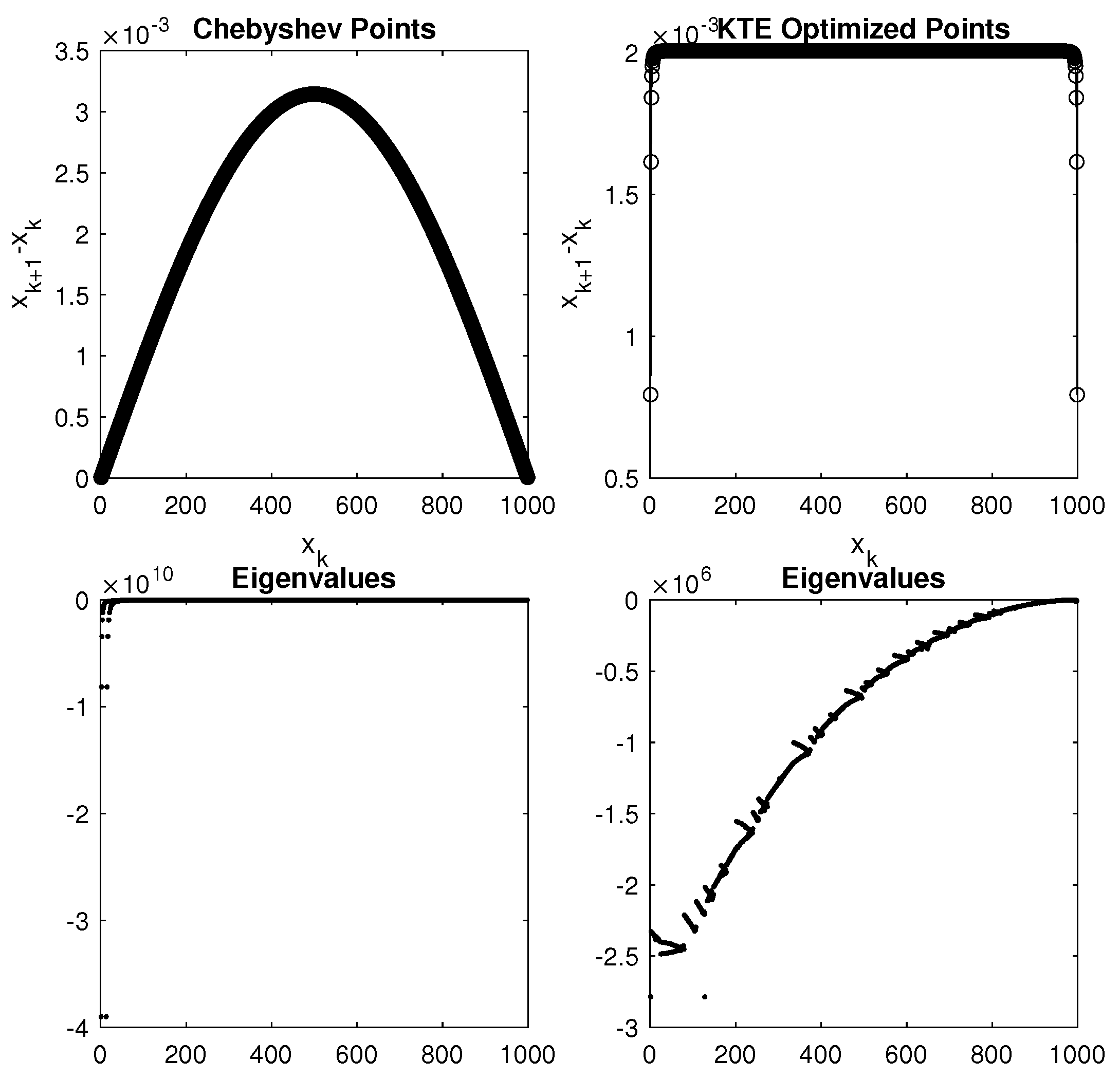
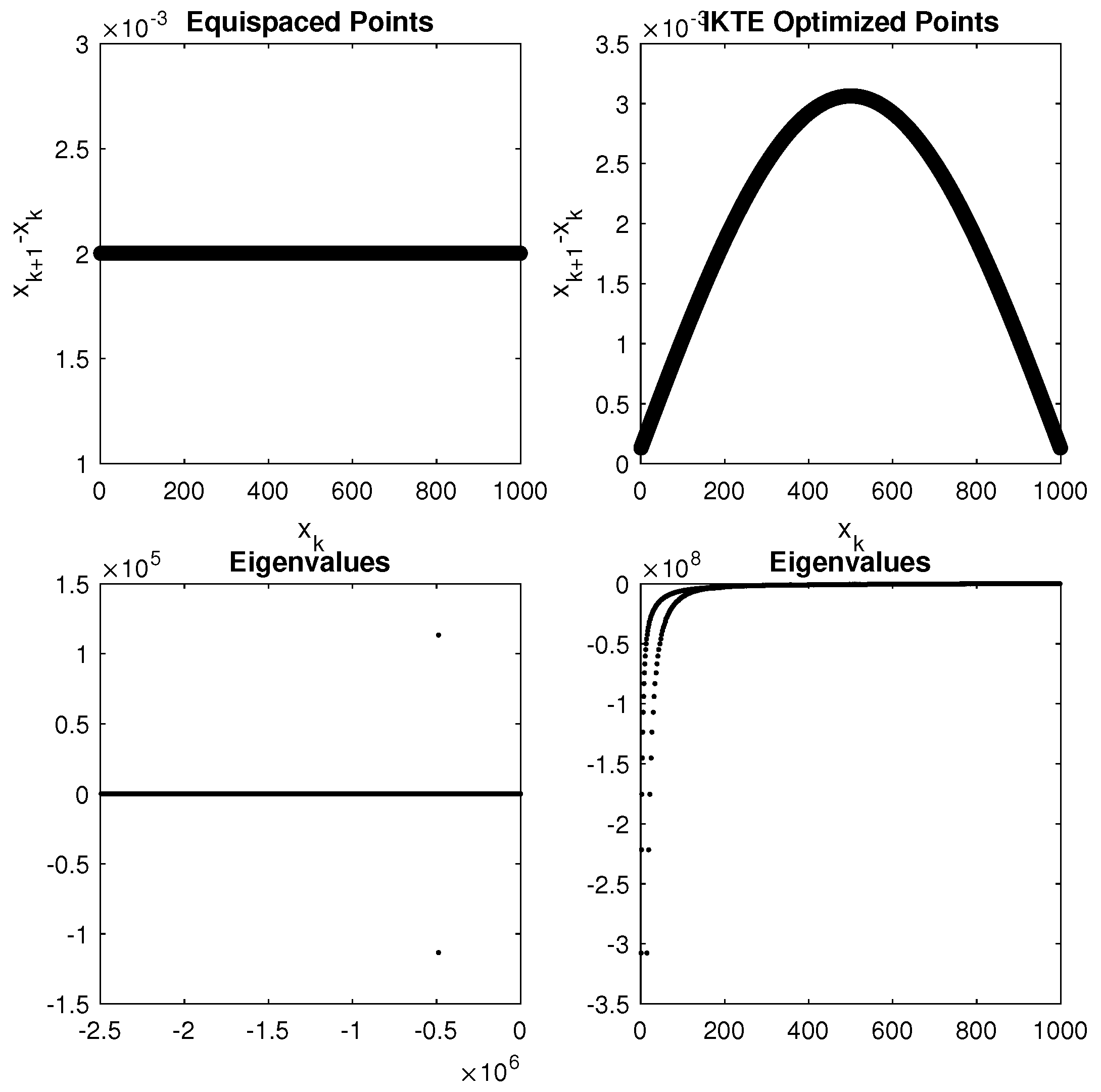
For example, we consider a 37 point stencil, ϕ r = r 5 , polynomials up to degree p = 14 , and 1000 nodes on the interval [ 1 , 1 ] for RBF-FD calculations. For the KTE and IKTE mapping, we use MATLAB’s fmincon to find the α that minimizes the Lebesgue constant. For the KTE mapping, we plot the inputted Chebyshev points and the resulting Dirichlet Laplacian eigenvalues on the left column of Figure 5. The spacing for the points resulting from finding the α that minimizes the Lebesgue constant and the corresponding Dirichlet Laplacian eigenvalues are depicted in the right column of Figure 5. In this case, the Lebesgue constant for the Chebyshev points and the mapped points are Λ R B F F D = 2.69 and Λ R B F F D = 1.82 , respectively. We notice that in this case, the mapped points are equispaced away from the boundary and become clustered close to the boundary. Both sets of points have negative, real eigenvalues; however, the mapped points have eigenvalues of smaller magnitude due to having a larger minimum spacing than the Chebyshev points.
Alternatively, we plot the results for the IKTE mapping in Figure 6. We notice that for equispaced points, the eigenvalues are imaginary. After using the IKTE mapped points, the eigenvalues return to being purely real. In this case, the Lebesgue constant for the equispaced points and the mapped points are Λ R B F F D = 4.59 and Λ R B F F D = 1.82 , respectively.
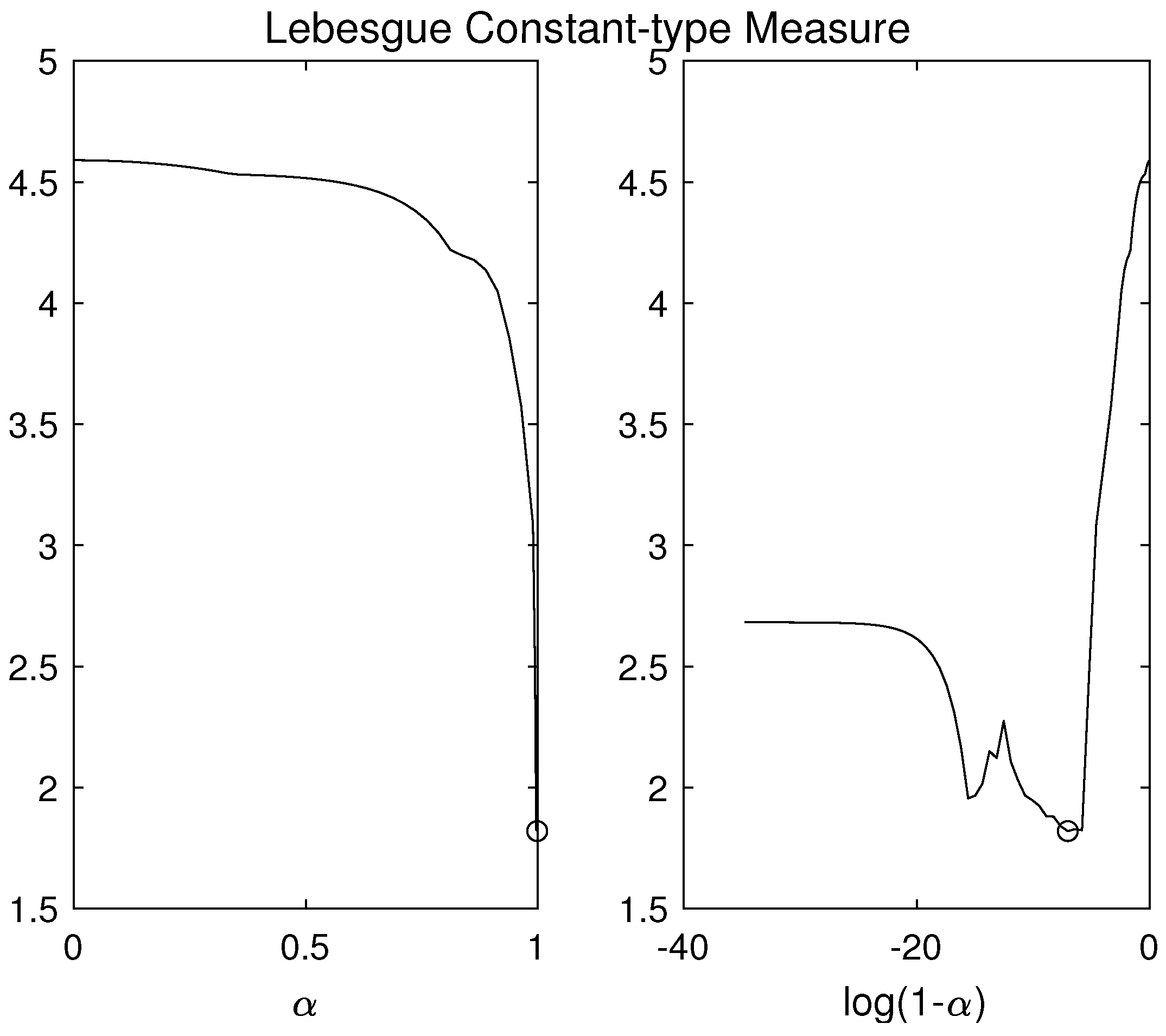
One thing we notice is that α that minimizes Λ R B F F D is very close to 1 from both mappings. That is, the KTE mapping maps the Chebyshev points to points close to equispaced points, and the IKTE mapping maps the equispaced points to points close to the Chebyshev points. This behavior illustrates the fact that the two mappings impact the behavior of clustering near the boundary in different ways, depending on what set of points is being inputted. Figure 7 illustrates the behavior of Λ R B F F D for different values of α using the IKTE mapping. The subfigure on the right uses a log scale for α to illustrate the behavior of Λ R B F F D for α close to 1. The optimal α is circled.
The results from the KTE and IKTE mapping in this case lead us to conclude that some clustering near the boundary gives the best results due to the fact that the equispaced points lead to eigenvalues with a non-zero imaginary part, while both mapped sets lead to purely real eigenvalues. Although the KTE and IKTE mappings inform the behavior of the placement of nodes for RBF-FD methods by tuning just one parameter, these mappings cannot be translated to 2D complex regions. As a result, we need a robust algorithm for placing points near the boundary in 2D: the MCpQR algorithm.

4.2. MCpQR Algorithm Point Sets

Based on the results in Section 4.1, we see that a set of points that are equispaced in most of the domain and clustered close to the boundary provide better eigenvalues. As a result, we would like to be able to generate a similar point set using the MCpQR algorithm. This algorithm would then be used to generate point sets for complex 2D regions.
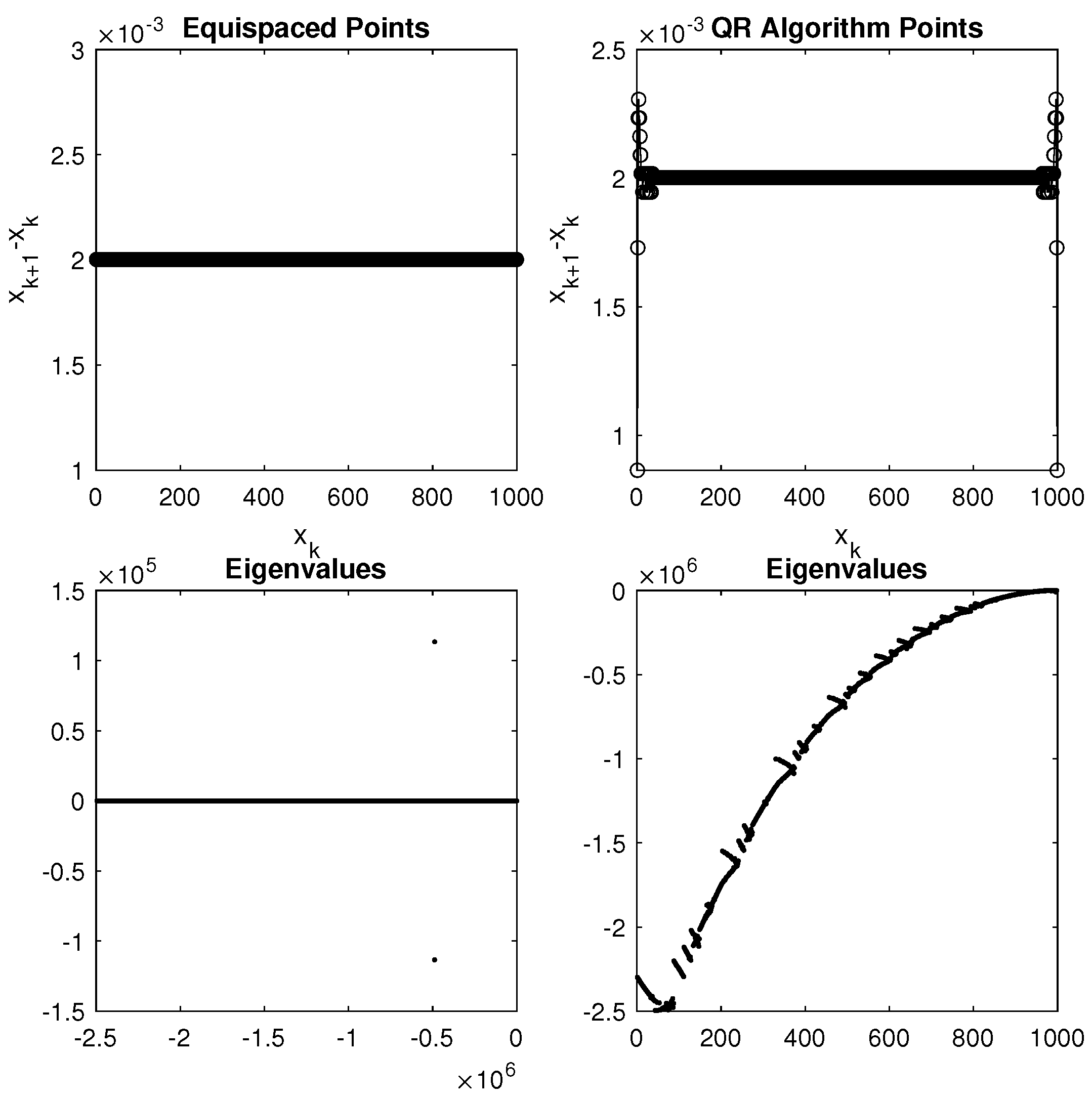
Using the same selections for PHS, polynomial degree, stencil size, and number of points as used in Section 4.1, we implement the MCpQR algorithm to compute point locations for RBF-FD methods. As mentioned previously, we require a starting guess of points to populate the piecewise cardinal function basis. Naturally, from the results Section 4.1, we use the equispaced points as the starting guess. The spacing for the points computed by the MCpQR algorithm along with the Dirichlet Laplacian eigenvalues are plotted in Figure 8. We notice that the algorithm is again able to compute points with purely real eigenvalues. The eigenvalues closely resemble those from the KTE mapping in Figure 5. In this case, we achieve Λ R B F F D = 1.85
We notice that the points computed by the MCpQR algorithm are again near-equispaced for most of the domain and clustered close to the boundary. One way to decrease unnecessary computational costs is to optimize only the points close to the end points of the domain. Thus, we choose a set of equispaced points away from the boundary and keep them fixed. Then, we can choose the spacing of the points near the boundary using our novel algorithm. The candidate points are populated only near the boundary, eliminating the need to incorporate candidate points on the majority of the [ 1 , 1 ] interval. This greatly reduces the computational costs outlined for the QR factorization in Section 3.2. Figure 9 illustrates the resulting point set when implementing this boundary-restricted approach. Starting with 1000 equispaced points, we restrict the 1000 2 k interior points and allow the k points closest to 1 and 1 to be moved. The resulting points achieve Λ R B F F D = 1.85 , the same value that resulted from an unrestricted algorithm. Additionally, we notice that the spacing near the boundary and eigenvalues are similar to the unrestricted algorithm. Thus, we are able to obtain these points for RBF-FD methods by just moving selecting points near the boundary using the MCpQR algorithm.

5. Results in 2D

Following the results in 1D, we naturally progress to point sets for RBF-FD methods in 2D. The MCpQR algorithm can be used in 2D as long as we have the required basis and candidate points. We begin with rectangular domains and follow with more complex 2D regions. We will demonstrate that the MCpQR algorithm provides a simple, robust algorithm for finding point sets for RBF-FD methods with reduced computational cost.

5.1. Unit Square Results

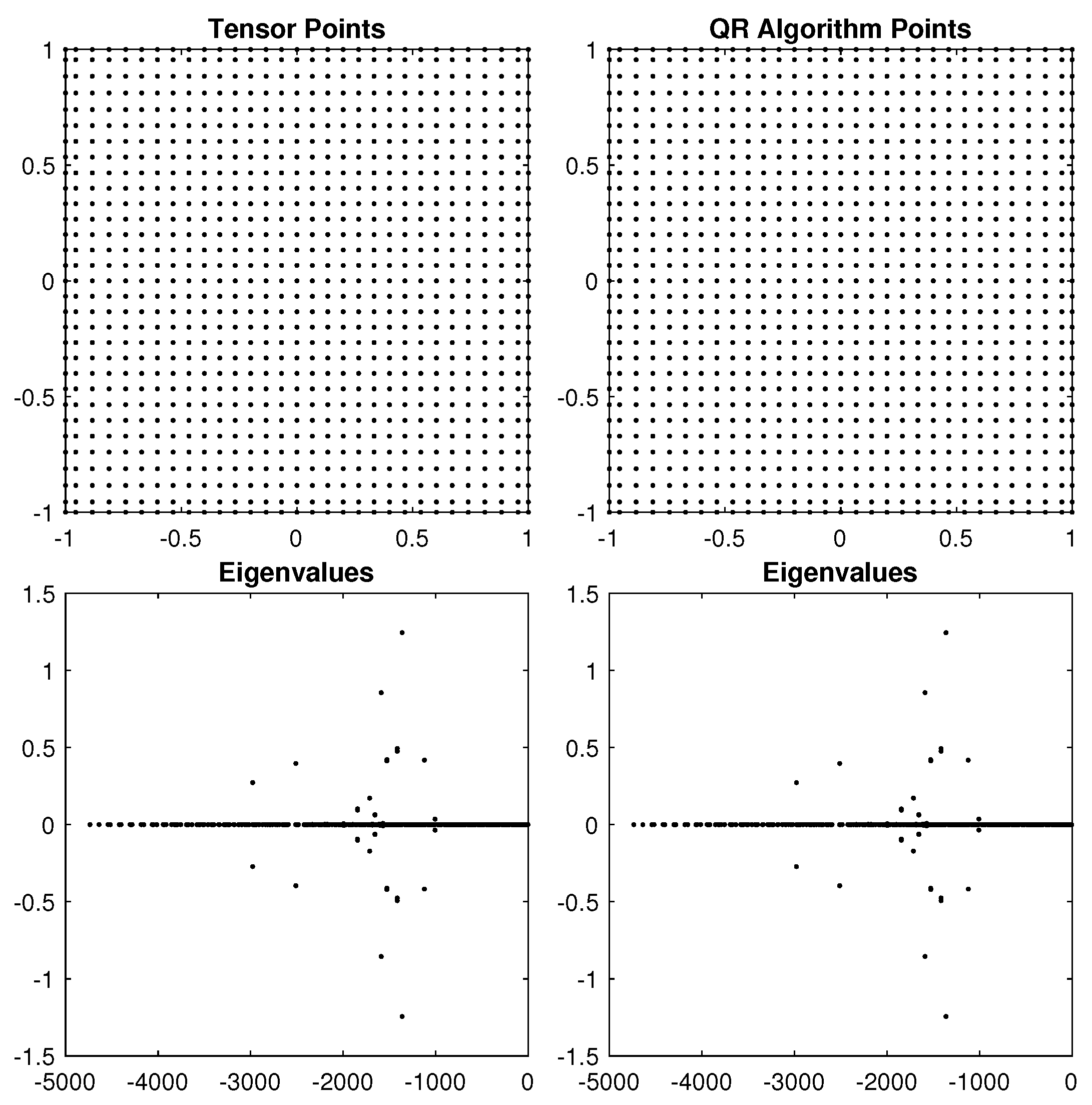
The first 2D region we consider is the unit square. The unit square allows us to consider the tensor product of resulting 1D point sets. We consider again a 37-point stencil, ϕ r = r 5 , polynomials up to degree p = 4 , and 961 nodes on the interval for RBF-FD calculations. In this case, the 961 nodes are a tensor product of 31 nodes on the [ 1 , 1 ] interval. Polynomials up to degree p = 4 append 15 polynomial basis functions, the same number appended for polynomials up to degree 14 in 1D. Figure 10, Figure 11 and Figure 12 plot the resulting QR algorithm points when using tensor product 1D points, hexagonal points, and scattered points as starting guesses. The tensor product 1D points are obtained by taking the tensor product of the points found using the QR algorithm in 1D, as shown in Figure 9.
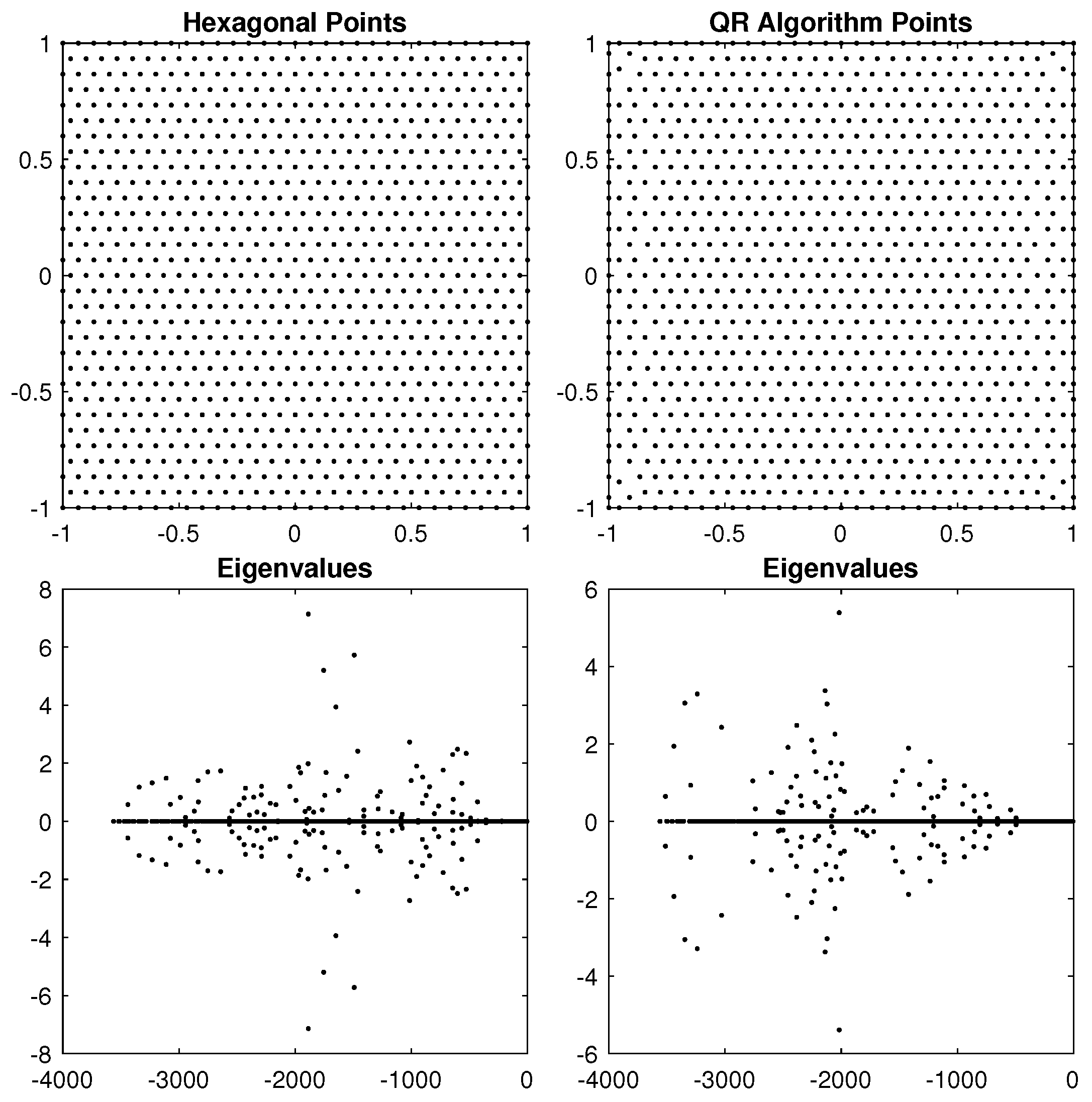
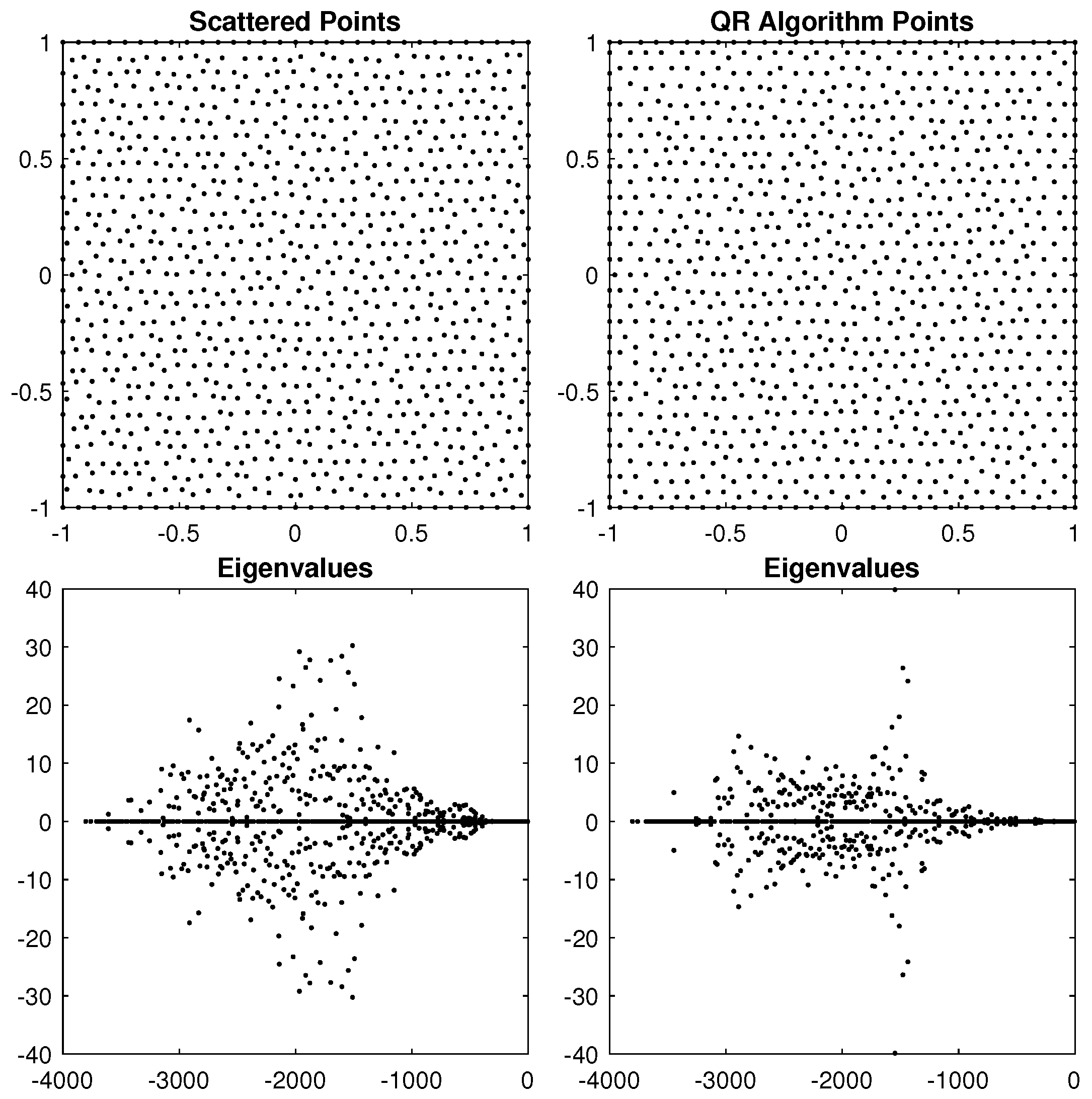
We notice that for explicit time-stepping, the hexagonal points and the scattered points provide the best eigenvalues. Using these sets for starting guesses, the MCpQR algorithm moves the points near the boundary to decrease the Lebesgue constant while preserving the general behavior of the eigenvalues. This is important, as for complex regions, we can place the hexagonal points within the complex region, draw the boundary of the complex region and move the points near the boundary with the algorithm. This will provide a method similar to the algorithm used to obtain scattered points for complex regions. We note that the tensor product points result in less optimal eigenvalues. The MCpQR algorithm does not move the points near the boundaries for these sets. Thus, these point sets should not be considered.
In Figure 13, we implement the MCpQR algorithm without fixing any nodes. The closely matched results from Figure 11 and Figure 13 show that limiting the algorithm to just moving the points near the boundary produces adequate point sets while eliminating the computational costs required by moving points both close to and away from the boundary. We notice that the points obtained from the MCpQR algorithm strongly depend on the starting guess. Thus, we can conclude from this that the points from the QR algorithm can only be considered as local minima, not global minima.
Next, we investigate the behavior of point sets for complex 2D regions. For complex regions, we consider the scattered points along with the points resulting from inputting hexagonal points into the QR algorithm since these two sets performed the best on the unit square. We notice three key benefits of using the MCpQR algorithm to generate points for RBF-FD methods in the examples above.
First, the robustness and simplicity of the algorithm allow us to easily generate point sets for any given region. As mentioned previously, the only requirements are a given basis and a set of candidate points. The only tunable parameters in this case are how many candidate points to use since the RBF-FD method already determines the basis used.
Second, in this case, the MCpQR algorithm-generated points produced eigenvalues with smaller imaginary parts. Thus, these points produced eigenvalues closer to the true Dirichlet Laplacian eigenvalues. This implies that for convective PDEs, less hyperviscosity may be needed to be applied in order to handle spurious eigenvalues that arise from the imaginary parts of the Dirichlet Laplacian.
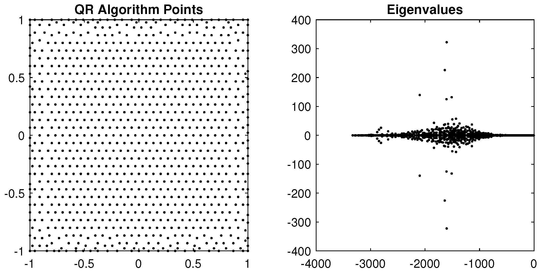
Lastly, the points generated by the MCpQR algorithm allow for a decrease in the stencil size requirements for RBF-FD methods. It has been previously recommended that stencil sizes be at least twice the number of polynomial basis functions appended. Thus, for the example used for the unit square, the stencil size should contain at least 30 points to maintain the conditioning of the system in Equation (5). The use of the points generated by the MCpQR algorithm alleviates the stencil size requirement. For this example, we are able to find points for the RBF-FD method that allow for the use of a 19 point stencil. This is done by first starting with a hexagonal point set using an adequate stencil size (30 in this example), performing the MCpQR algorithm, and using the resulting set as the starting guess to again run the MCpQR algorithm but now with a smaller stencil size. This is then iterated until the conditioning of the system degrades. The resulting point set for a 19 point stencil is shown in Figure 14.

5.2. Complex 2D Regions

We adapt the MCpQR algorithm to generate point sets for RBF-FD methods on complex 2D regions. We employ the same strategy: determine a starting point set, fix the interior nodes, and implement the MCpQR algorithm to choose the location of points near the boundary. We use the hexagonal points as the starting guess for the MCpQR algorithm since these points were shown to perform the best in Section 5.1.
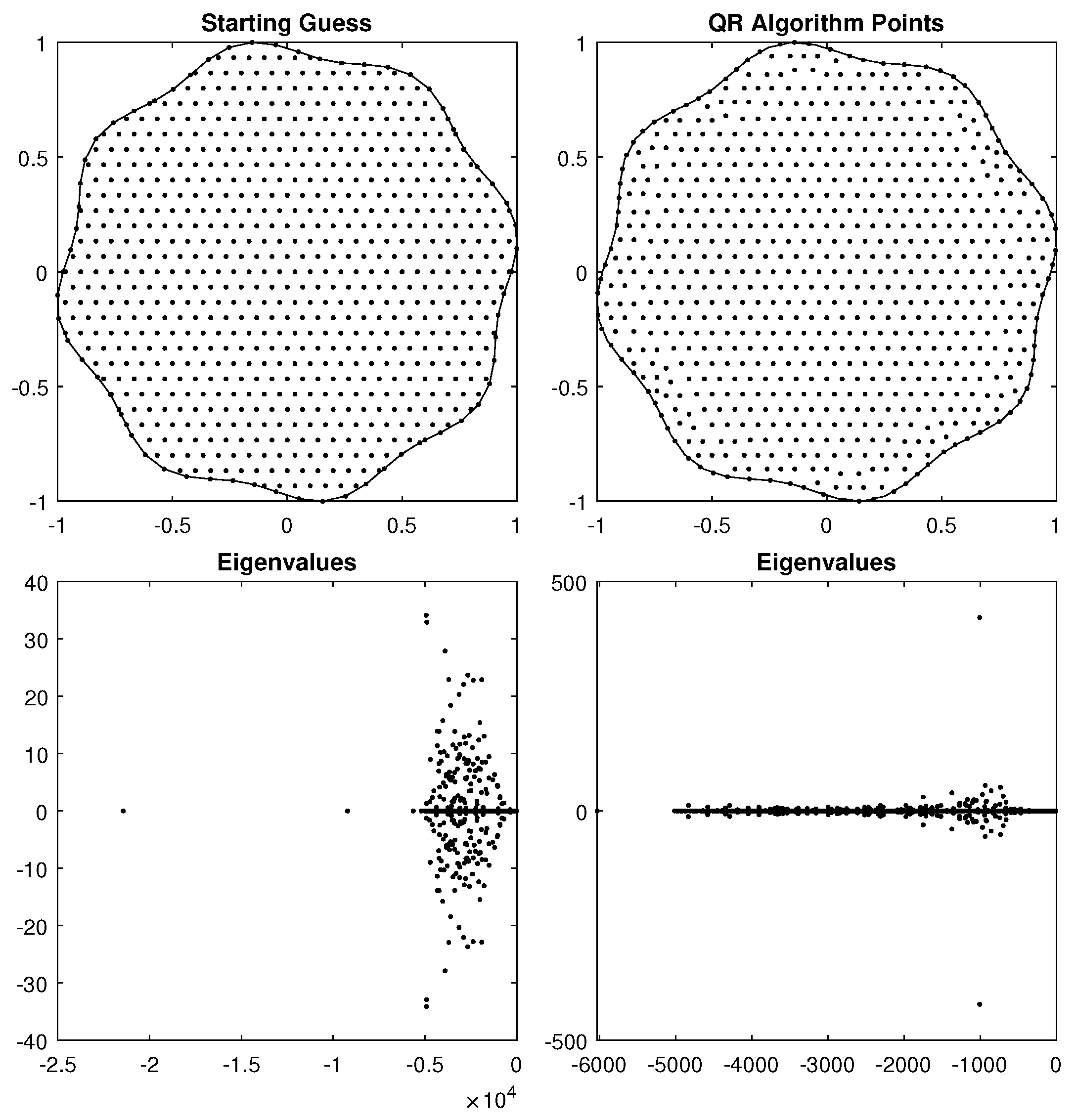
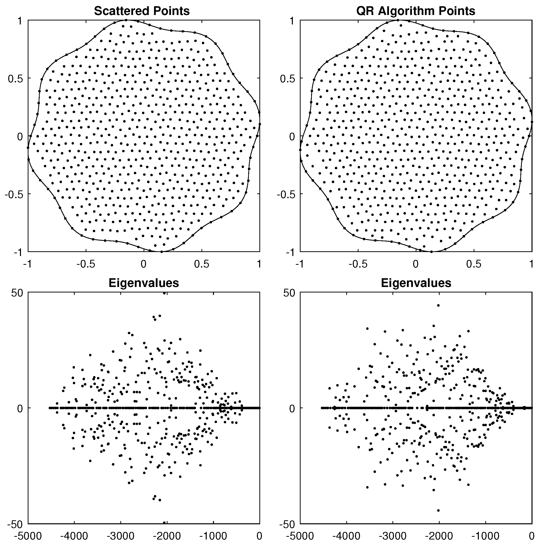
For complex regions, we populate the hexagonal points on the unit square, draw the complex region, and keep only the points lying on the interior of the shape. The boundary points of the complex region are then appended to the point set used as the starting guess. In Figure 15, both the starting guess and the resulting MCpQR algorithm sampling nodes for the bumped-disk region are plotted, along with their respective Dirichlet Laplacian eigenvalues. This case considers the bumped-disk region using a 37 point stencil, ϕ r = r 3 , and polynomials up to degree p = 4 . In this example, 734 nodes are used for RBF-FD calculations.
We note that the described method for populating the initial guess produces points that lie too close to each other. This occurs when the boundary points for the shape are located close to the hexagonal grid. As a result, the Dirichlet Laplacian eigenvalues are affected due to the close proximity of certain points. We notice that the MCpQR algorithm is able to remedy the clustering of points near the boundary and improve the behavior of the eigenvalues.
Figure 16 displays the results for another complex region: the peanut region. This example also considers a 37-point stencil, ϕ r = r 3 , and polynomials up to degree p = 4 . Here, 830 nodes are used for the RBF-FD calculations. Similar improvements in the spacing of points from the starting guess are observed.
We see that the strategy described in this section provides another method for populating point locations for RBF-FD methods on complex regions. The MCpQR algorithm is able to handle complex regions. Furthermore, as mentioned in Section 5.1, the MCpQR algorithm is able to be implemented with a few simple parameter selections (number of candidate points and basis) and allows for decreased computational costs as a result of lower stencil size requirements. Table 2 and Table 3 list the stencil size requirement improvement obtained by using the iteratively chosen points for different selections of polynomial degree and PHS degree for both the bumped-disk and peanut regions.
It should be noted that the MCcQR algorithm points and the scattered repel algorithm points perform similarly on complex regions with regards to stencil requirements and eigenvalue stability. Figure 17 plots the repel algorithm points on the bumped-disk region with ϕ r = r 3 and polynomials up to degree p = 3 . In this case, the repel algorithm points are able to handle a stencil size of 15 as well. Applying the MCpQR algorithm reduces the repel points starting guess measure from Λ R B F F D = 8.91 to Λ R B F F D = 3.56 ; however, there is no such improvement with regards to eigenvalue stability.
The 1D results from Section 4 suggest there should be some point clustering near the boundary of the region. It seems the MCpQR algorithm is not able to recreate the same behavior from 1D in 2D complex regions. After inputting the repel algorithm points (a quasi-uniformly distributed set with no clustering near the boundary) as a starting guess, the MCpQR does not improve the eigenvalues. This may be due to the fact that the algorithm is generating ’local minima’ type point sets. As a result, it is concluded that these repel algorithm points perform well on 2D complex regions.
One major benefit the MCpQR algorithm can provide on complex 2D regions is boundary point selection. Currently, the repel algorithm discretizes an equispaced boundary and keeps the boundary points fixed throughout the algorithm [4]. In this case, the algorithm does not inform any selection of boundary points. The MCpQR algorithm can be used in conjunction with the repel algorithm to identify which boundary points to use along with the interior points resulting from the repel algorithm. Consider the bumped-disk region using a 37-point stencil, ϕ r = r 3 , and polynomials up to degree p = 4 . In Figure 18, we see that if we implement the scattered repel algorithm points with too few points on the boundary, the MCqQR algorithm selects additional points to place on the boundary. In this case, the number of boundary points increases from 31 to 63. We notice the improvement in the imaginary part of the eigenvalues. Thus, the MCpQR algorithm can be applied to determine a minimum number of boundary points to use with the scattered repel algorithm points. This again improves eigenvalue stability while decreasing computational cost by keeping the number of boundary points to a minimum. Figure 19 illustrates the same results for the peanut region using a 37 point stencil, ϕ r = r 3 , and polynomials up to degree p = 4 . In this case, the number of boundary points increases from 31 to 68, and the same improvement in the imaginary part of the eigenvalues is observed. We see that the MCpQR algorithm can be used in conjunction with the scattered repel point algorithm to generate a set of boundary points along with a set of quasi-uniformly distributed interior points with reduced computational requirements and improved eigenvalue stability.

6. Test Cases Using MCpQR Algorithm Points

The accuracy of the RBF-FD method implemented with the optimized points is verified by finding the solution to test case PDEs. After implementing the MCpQR algorithm to find sampling points and differentiation matrices for the complex region (peanut and bumped-disk), Ω , we find the solution to each test case listed below. A fourth-order Runge–Kutta method is used for time-stepping.

6.1. Diffusion Equation with Forcing Term

The first test case involves finding the solution, u t , x , y , at time t = 10 for the following PDE:
u t = Δ u + sin t ,
u 0 = 0 ,
u Ω = 0 .
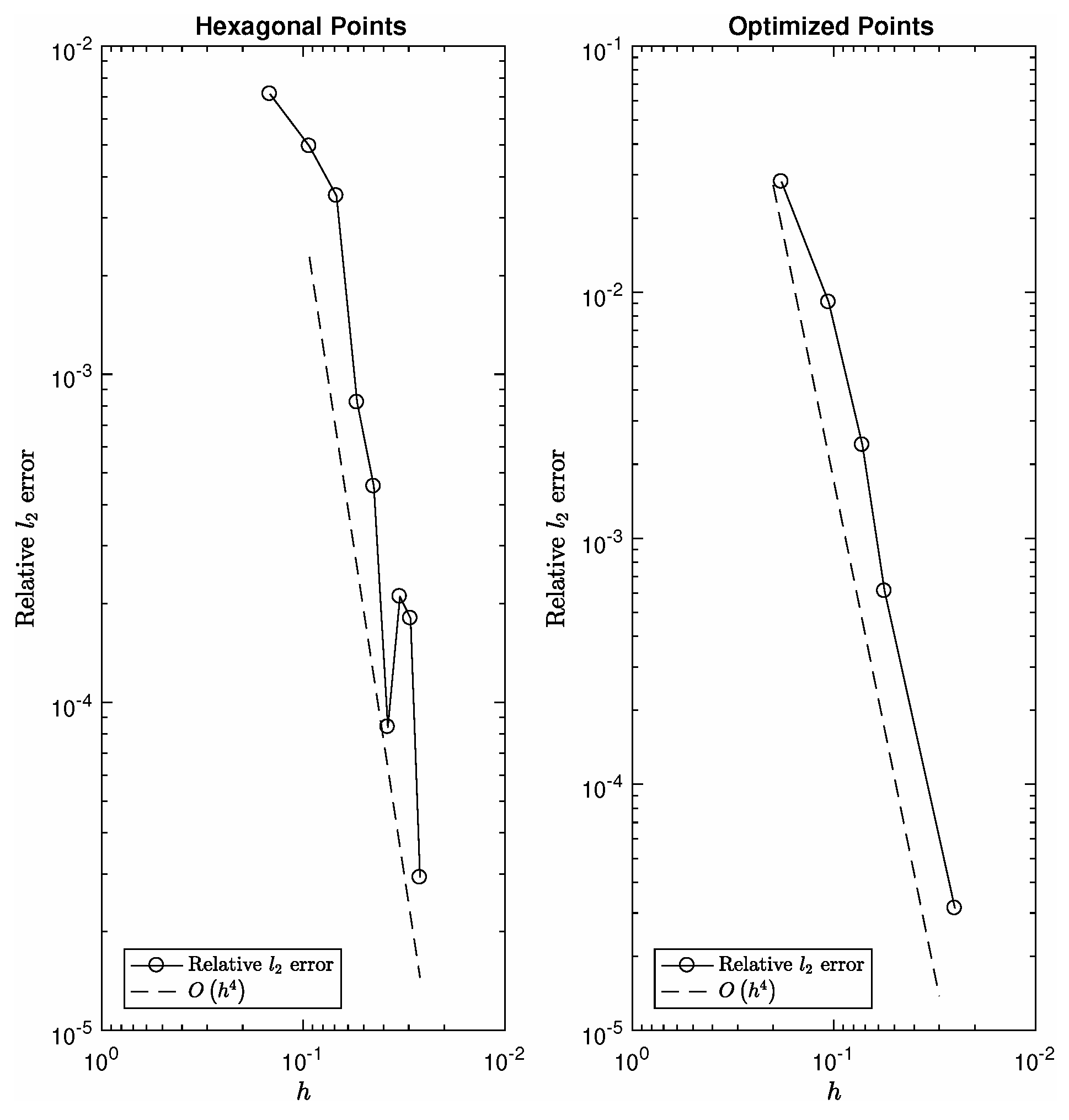
This test case is implemented using a 37-point stencil, ϕ r = r 3 , and polynomials of degree p = 4 . The expected rate of convergence is O h 4 since the rate is dependent on the degree of polynomials used. Running this test case, the same rate of convergence is observed with the optimized points. This is illustrated in Figure 20, which plots the relative error against the average spacing between each sampling point. In this case, a node refinement process is used, and the true solution is taken to be the solution resulting from the case using the finest spacing.

6.2. Wave Equation with Hyperviscosity

The second test case requires the implementation of the hyperviscosity methods. This case involves finding the solution, u t , x , y , at time t = 20 for the following PDE:
u t t = Δ u ,
u 0 = f x , y ,
u t 0 = 0 ,
u Ω = 0 .
Hyperviscosity methods were first introduced in [39] and further studied in [40,41]. These methods allow stable numerical time-stepping for RBF-FD methods. Without hyperviscosity, the differentiation matrices for convective PDEs using RBF-FD methods presented spurious eigenvalues. By damping the spurious eigenvalues while simultaneously preserving the relevant physical properties, the hyperviscosity methods effectively achieve stable numerical time-stepping while still preserving accuracy in the PDE solutions.
The point sets from the MCpQR algorithm are used for hyperviscosity methods. Implementing hyperviscosity methods requires the approximation of high order powers of the Laplacian operator to use as a filter for stable time-stepping. The technique is to then add the high order Laplacian operator to the governing equation of the PDE. As a result, spurious eigenvalues existing in the right (positive, real) half-plane are then shifted into the left (negative, real) half-plane.
Consider the following setup:
u v t = L u v ,
where L is some operator whose differentiation matrix, obtained by implementing RBF-FD methods with PHSs and polynomials, contains spurious eigenvalues. The hyperviscosity method is implemented by redefining the system as:
u v t = L u v + 1 K + 1 γ h 2 K 1 Δ k u Δ k v ,
where k denotes the order of the Laplacian used in the hyperviscosity implementation, h represents the average node-spacing, and γ is a parameter that tunes the hyperviscosity filter.
It is important to select a suitable value for the parameter γ . If γ is chosen to be too large, the eigenvalues are forced further out in the left half-plane. Thus, the solution to the PDE will be limited to smaller time-stepping. Furthermore, large values of γ may end up filtering the physically relevant lower modes, thereby, creating accuracy errors. If the hyperviscosity parameter is chosen to be too small, then the possibility of still having eigenvalues existing in the right half-plane, and thus generating an unstable method, remains.
To approximate the higher order Laplacian operators, Gaussian RBFs, ϕ r = e ε r 2 , are used due to the simplicity of higher order Laplacian formulas, which are generalized in [20]. In the case of 2D complex regions, the operators can be approximated by:
Δ 0 ϕ r = ϕ r ,
Δ 1 ϕ r = ε 2 4 ε r 2 4 ϕ r ,
Δ 2 ϕ r = ε 4 16 ε r 4 64 ε r 2 + 32 ϕ r ,
Δ 3 ϕ r = ε 6 64 ε r 6 576 ε r 4 + 1152 ε r 2 384 ϕ r .
The hyperviscosity system for the PDE described in Equations (18)–(21) is then defined as:
u v t = 1 K + 1 γ h 2 K 1 Δ k I Δ 1 K + 1 γ h 2 K 1 Δ k u v , = L ^ u v ,
where v = u t .
This test case is implemented using a 28-point stencil, ϕ r = r 9 , polynomials of degree p = 4 , and Δ 3 -type hyperviscosity. Again, the expected rate of convergence is O h 4 since the rate is dependent on the degree of polynomials used. Running this test case, the O h 4 rate of convergence is again observed with the optimized points. This is illustrated in Figure 21, where we plot the relative error against the average spacing between each sampling point. For this example, a Bessel function of the first kind on the unit disk is used to provide the initial and boundary conditions. The relative error is then calculated using an exact solution to the PDE.

7. Conclusions

A piecewise-defined Lebesgue constant for RBF-FD methods is introduced. Based on the commonly used Lebesgue constant for polynomial interpolation, this measure allows us to sample points for RBF-FD methods combining PHSs and polynomials. We studied the behavior of point sets in 1D, simple 2D regions, and complex 2D regions. Points were generated by modifying a column-pivoting QR algorithm previously used to find optimal points for polynomial interpolation. The resulting points mitigate stencil size restrictions resulting from the use of RBF-FD methods, thus reducing computational cost while preserving accuracy and convergence properties. This method also provides a simple, robust algorithm for point generation with few parameters needing to be tuned. Lastly, we implement the MCpQR algorithm to inform the location of boundary points to be used in conjunction with the scattered repel algorithm points. In the future, 3D regions may be considered as well. One framework for a 3D application is given in [42]. The column-pivoting QR algorithm may be modified to handle RBF-FD methods for 3D by appending corresponding polynomial bases.

Author Contributions

Conceptualization, R.B.P.; Investigation, T.L.; Software, T.L.; Supervision, R.B.P.; Validation, T.L.; Visualization, T.L.; Writing—original draft, T.L.; Writing—review and editing, T.L. All authors have read and agreed to the published version of the manuscript.

Funding

This research received no external funding.

Institutional Review Board Statement

Not applicable.

Informed Consent Statement

Not applicable.

Data Availability Statement

Not applicable.

Acknowledgments

Tony Liu was sponsored by the National Science Foundation (DMS-1502640) for the duration of this work. The authors would like to acknowledge Victor Bayona for providing his code on scattered node generation based on repel algorithms.

Conflicts of Interest

The authors declare no conflict of interest.

References

  1. Barnett, G. A Robust RBF-FD Formulation Based on Polyharmonic Splines and Polynomials. Ph.D. Thesis, University of Colorado Boulder, Boulder, CO, USA, 2015. [Google Scholar]
  2. Barnett, G.A.; Flyer, N.; Wicker, L.J. An RBF-FD polynomial method based on polyharmonic splines for the Navier-Stokes equations: Comparisons on different node layouts. arXiv 2015, arXiv:1509.02615. [Google Scholar]
  3. Bayona, V.; Flyer, N.; Fornberg, B. On the role of polynomials in RBF-FD approximations: III. Behavior near domain boundaries. J. Comput. Phys. 2019, 380, 378–399. [Google Scholar] [CrossRef] [Green Version]
  4. Bayona, V.; Flyer, N.; Fornberg, B.; Barnett, G.A. On the role of polynomials in RBF-FD approximations: II. Numerical solution of elliptic PDEs. J. Comput. Phys. 2017, 332, 257–273. [Google Scholar] [CrossRef] [Green Version]
  5. Flyer, N.; Barnett, G.A.; Wicker, L.J. Enhancing finite differences with radial basis functions: Experiments on the Navier-Stokes equations. J. Comput. Phys. 2016, 316, 39–62. [Google Scholar] [CrossRef] [Green Version]
  6. Flyer, N.; Fornberg, B.; Bayona, V.; Barnett, G.A. On the role of polynomials in RBF-FD approximations: I. Interpolation and accuracy. J. Comput. Phys. 2016, 321, 21–38. [Google Scholar] [CrossRef] [Green Version]
  7. Fasshauer, G.E.; Zhang, J.G. On choosing “optimal” shape parameters for RBF approximation. Numer. Algorithms 2007, 45, 345–368. [Google Scholar] [CrossRef]
  8. Mongillo, M. Choosing basis functions and shape parameters for radial basis function methods. SIAM Undergrad. Res. Online 2011, 4, 2–6. [Google Scholar] [CrossRef]
  9. Hagstrom, T.; Hagstrom, G. Grid stabilization of high-order one-sided differencing I: First-order hyperbolic systems. J. Comput. Phys. 2007, 223, 316–340. [Google Scholar] [CrossRef]
  10. Hagstrom, T.; Hagstrom, G. Grid stabilization of high-order one-sided differencing II: Second-order wave equations. J. Comput. Phys. 2012, 231, 7907–7931. [Google Scholar] [CrossRef]
  11. Hermanns, M.; Hernández, J.A. Stable high-order finite-difference methods based on non-uniform grid point distributions. Int. J. Numer. Methods Fluids 2008, 56, 233–255. [Google Scholar] [CrossRef] [Green Version]
  12. Zhong, X.; Tatineni, M. High-order non-uniform grid schemes for numerical simulation of hypersonic boundary-layer stability and transition. J. Comput. Phys. 2003, 190, 419–458. [Google Scholar] [CrossRef]
  13. Slak, J.; Kosec, G. On generation of node distributions for meshless PDE discretizations. SIAM J. Sci. Comput. 2019, 41, A3202–A3229. [Google Scholar] [CrossRef] [Green Version]
  14. Fornberg, B.; Flyer, N. Fast generation of 2D node distributions for mesh-free PDE discretizations. Comput. Math. Appl. 2015, 69, 531–544. [Google Scholar] [CrossRef]
  15. van der Sande, K.; Fornberg, B. Fast variable density 3-D node generation. arXiv 2019, arXiv:1906.00636. [Google Scholar]
  16. Shankar, V.; Kirby, R.M.; Fogelson, A.L. Robust node generation for mesh-free discretizations on irregular domains and surfaces. SIAM J. Sci. Comput. 2018, 40, A2584–A2608. [Google Scholar] [CrossRef] [Green Version]
  17. Wendland, H. Scattered Data Approximation; Cambridge University Press: Cambridge, UK, 2004; Volume 17. [Google Scholar]
  18. Fasshauer, G.E. Meshfree Approximation Methods with Matlab:(With CD-ROM); World Scientific Publishing Co Inc.: Hackensack, NJ, USA, 2007; Volume 6. [Google Scholar]
  19. Flyer, N.; Wright, G.B.; Fornberg, B. Radial basis function-generated finite differences: A mesh-free method for computational geosciences. Handb. GeoMath. Springer Ref. 2014, 130, 1–30. [Google Scholar]
  20. Fornberg, B.; Flyer, N. A Primer on Radial Basis Functions with Applications to the Geosciences; SIAM: Philadelphia, PA, USA, 2015. [Google Scholar]
  21. Shankar, V. The overlapped radial basis function-finite difference (RBF-FD) method: A generalization of RBF-FD. J. Comput. Phys. 2017, 342, 211–228. [Google Scholar] [CrossRef] [Green Version]
  22. Bayona, V. Comparison of moving least squares and RBF+ poly for interpolation and derivative approximation. J. Sci. Comput. 2019, 81, 486–512. [Google Scholar] [CrossRef]
  23. Bos, L.; Calvi, J.P.; Levenberg, N.; Sommariva, A.; Vianello, M. Geometric weakly admissible meshes, discrete least-squares approximations and approximate Fekete points. Math. Comput. 2011, 80, 1623–1638. [Google Scholar] [CrossRef]
  24. Bos, L.; De Marchi, S.; Sommariva, A.; Vianello, M. Computing multivariate Fekete and Leja points by numerical linear algebra. SIAM J. Numer. Anal. 2010, 48, 1984–1999. [Google Scholar] [CrossRef] [Green Version]
  25. Bos, L.; Levenberg, N. On the calculation of approximate Fekete points: The univariate case. Electron. Trans. Numer. Anal. 2008, 30, 377–397. [Google Scholar]
  26. Briani, M.; Sommariva, A.; Vianello, M. Computing Fekete and Lebesgue points: Simplex, square, disk. J. Comput. Appl. Math. 2012, 236, 2477–2486. [Google Scholar] [CrossRef]
  27. Caliari, M.; De Marchi, S.; Vianello, M. Bivariate polynomial interpolation on the square at new nodal sets. Appl. Math. Comput. 2005, 165, 261–274. [Google Scholar] [CrossRef]
  28. Gunzburger, M.; Teckentrup, A.L. Optimal point sets for total degree polynomial interpolation in moderate dimensions. arXiv 2014, arXiv:1407.3291. [Google Scholar]
  29. Guo, L.; Narayan, A.; Yan, L.; Zhou, T. Weighted approximate Fekete points: Sampling for least-squares polynomial approximation. arXiv 2017, arXiv:1708.01296. [Google Scholar] [CrossRef] [Green Version]
  30. Narayan, A.; Xiu, D. Stochastic collocation methods on unstructured grids in high dimensions via interpolation. SIAM J. Sci. Comput. 2012, 34, A1729–A1752. [Google Scholar] [CrossRef]
  31. Narayan, A.; Xiu, D. Constructing Nested Nodal Sets for Multivariate Polynomial Interpolation. SIAM J. Sci. Comput. 2013, 35, A2293–A2315. [Google Scholar] [CrossRef]
  32. Sommariva, A.; Vianello, M. Computing approximate Fekete points by QR factorizations of Vandermonde matrices. Comput. Math. Appl. 2009, 57, 1324–1336. [Google Scholar] [CrossRef] [Green Version]
  33. Van Barel, M.; Humet, M.; Sorber, L. Approximating optimal point configurations for multivariate polynomial interpolation. Electron. Trans. Numer. Anal. 2014, 42, 41–63. [Google Scholar]
  34. Shukla, R.K.; Zhong, X. Derivation of high-order compact finite difference schemes for non-uniform grid using polynomial interpolation. J. Comput. Phys. 2005, 204, 404–429. [Google Scholar] [CrossRef]
  35. Kosloff, D.; Tal-Ezer, H. A modified Chebyshev pseudospectral method with an O(N-1) time step restriction. J. Comput. Phys. 1993, 104, 457–469. [Google Scholar] [CrossRef]
  36. Platte, R.B. How fast do radial basis function interpolants of analytic functions converge? IMA J. Numer. Anal. 2011, 31, 1578–1597. [Google Scholar] [CrossRef] [Green Version]
  37. Li, T.; Pintus, N.; Viglialoro, G. Properties of solutions to porous medium problems with different sources and boundary conditions. Z. FÜR Angew. Math. Und Phys. 2019, 70, 1–18. [Google Scholar] [CrossRef] [Green Version]
  38. Marras, M.; Piro, S.V.; Viglialoro, G. Lower bounds for blow-up time in a parabolic problem with a gradient term under various boundary conditions. Kodai Math. J. 2014, 37, 532–543. [Google Scholar] [CrossRef]
  39. Fornberg, B.; Lehto, E. Stabilization of RBF-generated finite difference methods for convective PDEs. J. Comput. Phys. 2011, 230, 2270–2285. [Google Scholar] [CrossRef]
  40. Larsson, E.; Lehto, E.; Heryudono, A.; Fornberg, B. Stable computation of differentiation matrices and scattered node stencils based on Gaussian radial basis functions. SIAM J. Sci. Comput. 2013, 35, A2096–A2119. [Google Scholar] [CrossRef] [Green Version]
  41. Shankar, V.; Fogelson, A.L. Hyperviscosity-based stabilization for radial basis function-finite difference (RBF-FD) discretizations of advection–diffusion equations. J. Comput. Phys. 2018, 372, 616–639. [Google Scholar] [CrossRef]
  42. Gunderman, D.; Flyer, N.; Fornberg, B. Transport schemes in spherical geometries using spline-based RBF-FD with polynomials. J. Comput. Phys. 2020, 408, 109256. [Google Scholar] [CrossRef]
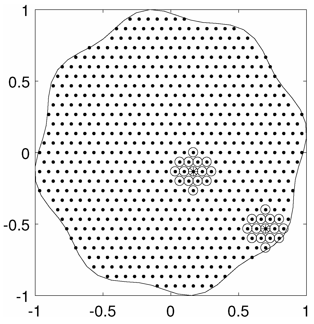
Figure 1. Fifteen-node stencil example for the bumped-disk region.
Mathematics 09 01845 g001
Figure 2. Convergence rates of a first-order derivative approximation using PHS and polynomials.
Mathematics 09 01845 g002
Figure 3. Stencil grouping example.
Mathematics 09 01845 g003
Figure 4. Piecewise cardinal function example. Clockwise starting from the top left:  l 1 x , l 2 x , l 4 x , l 3 x .
Mathematics 09 01845 g004
Figure 5. Chebyshev points, KTE optimized points, and their eigenvalues for a 37 point stencil with polynomials up to degree p = 15 . In this case, both point sets produce purely real eigenvalues.
Mathematics 09 01845 g005
Figure 6. Equispaced points, IKTE optimized points, and their eigenvalues for a 37-point stencil with polynomials up to degree p = 15 . The equispaced points produce complex eigenvalues, while the IKTE optimized points produce purely real eigenvalues.
Mathematics 09 01845 g006
Figure 7. Lebesgue constant for the IKTE mapped points using a 37-point stencil with polynomials up to degree p = 15 . The optimal α is circled.
Mathematics 09 01845 g007
Figure 8. MCpQR algorithm point spacing and Dirichlet Laplacian eigenvalues compared to equispaced points.
Mathematics 09 01845 g008
Figure 9. MCpQR algorithm point spacing and Dirichlet Laplacian eigenvalues compared to equispaced points. In this case, the majority of the points are fixed.
Mathematics 09 01845 g009
Figure 10. Tensor product points and resulting MCpQR algorithm points with Dirichlet Laplacian eigenvalues.
Mathematics 09 01845 g010
Figure 11. Hexagonal points and resulting MCpQR algorithm points with Dirichlet Laplacian eigenvalues.
Mathematics 09 01845 g011
Figure 12. Scattered points and resulting MCpQR algorithm points with Dirichlet Laplacian eigenvalues.
Mathematics 09 01845 g012
Figure 13. Hexagonal points and resulting MCpQR algorithm points with Dirichlet Laplacian eigenvalues. No interior points are fixed.
Mathematics 09 01845 g013
Figure 14. Resulting points for a 19-point stencil with Dirichlet Laplacian eigenvalues. These points were obtained by iteratively applying the MCpQR algorithm for smaller stencils.
Mathematics 09 01845 g014
Figure 15. Hexagonal points and resulting MCpQR algorithm points with Dirichlet Laplacian eigenvalues for the bumped-disk region.
Mathematics 09 01845 g015
Figure 16. Hexagonal points and resulting MCpQR algorithm points with Dirichlet Laplacian eigenvalues for the peanut region.
Mathematics 09 01845 g016
Figure 17. Scattered repel algorithm points and resulting MCpQR points with Dirichlet Laplacian eigenvalues.
Mathematics 09 01845 g017
Figure 18. MCpQR boundary selection for scattered repel algorithm points on the bumped-disk region.
Mathematics 09 01845 g018
Figure 19. MCpQR boundary selection for scattered repel algorithm points on the peanut region.
Mathematics 09 01845 g019
Figure 20. Solution convergence for the diffusion equation with forcing term using optimized points.
Mathematics 09 01845 g020
Figure 21. Solution convergence for the wave equation with hyperviscosity for hexagonal and optimized points.
Mathematics 09 01845 g021
Table 1. Example RBFs.
RBFBasis FunctionParameter
Polyharmonic Spline ϕ r = r m m 2 N 1
Multiquadric ϕ r = 1 + ε r 2 ε R
Inverse Multiquadric ϕ r = 1 1 + ε r 2 ε R
Gaussian ϕ r = e ε r 2 ε R
Table 2. Stencil size reduction for different selections of polynomial degree and PHS degree for the bumped-disk region.
Bumped-Disk Region, 734 Nodes
Polynomial DegreePHS DegreeTwo Times the Number of Polynomial Basis VectorsRequired Stencil Size (Optimized Pts)
deg = 3 r 3 k = 2015
deg = 3 r 5 k = 2015
deg = 3 r 7 k = 2015
deg = 4 r 3 k = 3019
deg = 4 r 5 k = 3021
deg = 4 r 7 k = 3021
deg = 5 r 3 k = 4231
deg = 5 r 5 k = 4231
deg = 5 r 7 k = 4227
Table 3. Stencil size reduction for different selections of polynomial degree and PHS degree for the peanut region.
Peanut Region, 830 Nodes
Polynomial DegreePHS DegreeTwo Times the Number of Polynomial Basis VectorsRequired Stencil Size (Optimized Pts)
deg = 3 r 3 k = 2015
deg = 3 r 5 k = 2015
deg = 3 r 7 k = 2015
deg = 4 r 3 k = 3021
deg = 4 r 5 k = 3025
deg = 4 r 7 k = 3025
deg = 5 r 3 k = 4231
deg = 5 r 5 k = 4231
deg = 5 r 7 k = 4233
Publisher’s Note: MDPI stays neutral with regard to jurisdictional claims in published maps and institutional affiliations.