Theory and Applications of the Unit Gamma/Gompertz Distribution

Abstract

Unit distributions are commonly used in probability and statistics to describe useful quantities with values between 0 and 1, such as proportions, probabilities, and percentages. Some unit distributions are defined in a natural analytical manner, and the others are derived through the transformation of an existing distribution defined in a greater domain. In this article, we introduce the unit gamma/Gompertz distribution, founded on the inverse-exponential scheme and the gamma/Gompertz distribution. The gamma/Gompertz distribution is known to be a very flexible three-parameter lifetime distribution, and we aim to transpose this flexibility to the unit interval. First, we check this aspect with the analytical behavior of the primary functions. It is shown that the probability density function can be increasing, decreasing, “increasing-decreasing” and “decreasing-increasing”, with pliant asymmetric properties. On the other hand, the hazard rate function has monotonically increasing, decreasing, or constant shapes. We complete the theoretical part with some propositions on stochastic ordering, moments, quantiles, and the reliability coefficient. Practically, to estimate the model parameters from unit data, the maximum likelihood method is used. We present some simulation results to evaluate this method. Two applications using real data sets, one on trade shares and the other on flood levels, demonstrate the importance of the new model when compared to other unit models.

1. Introduction

The development of unit distributions has accelerated significantly in recent years. They concentrate on modeling a wide range of events utilizing data with values between 0 and 1, including proportions, probabilities, and percentages, among other things. One reason is the growth of compositional data. On this subject, we can refer the reader to [1]. The construction of parametric, semi-parametric, and regression models is also a strong demand in applied fields for the analysis of such data in particular. The list of unit distributions is lengthy, and it continues to grow year after year. Most modern unit distributions are created by transforming existing distributions through suitably modified schemes. For example, if a random variable X has a lifetime distribution, the inverse-exponential scheme considers the random variable $Y=e^{-X}$ or $Y=e^{-\alpha x}$ with $\alpha >0$, which mechanically has a unit distribution. This particular scheme is also known to transpose some characteristics of the distribution of X to the unit interval. With this inverse-exponential scheme, we may refer the reader to the construction of the log-gamma distribution developed by [2] and based on the standard gamma distribution, log-Lindley distribution established by [3] and based on the Lindley distribution, unit Weibull distribution examined by [4,5] and using the Weibull distribution, unit Gompertz distribution developed by [6] and based on the Gompertz distribution, unit Burr-XII (UBXII) created by [7] distribution and based on the Burr-XII distribution, log-weighted exponential distribution motivated by [8] and based on the weighted exponential distribution, log-Xgamma distribution proposed by [9] and based on the Xgamma distribution, and unit Rayleigh (UR) distribution studied in [10] and using the Rayleigh distribution, among others.

Our study follows this spirit by considering a lifetime distribution never used in this context: the gamma/Gompertz (G/G) distribution. To begin with, the G/G distribution is a three-parameter continuous probability distribution introduced in probability and statistics by [11]. It was first used as a customer lifetime model and an aggregate model of mortality risks. From the mathematical side, the cumulative distribution function (cdf) defining the G/G distribution is

$$\begin{array}{c}\hfill F_{G/G}(x;b,s,\beta )=1-\frac{{\beta }^s}{{(\beta -1+e^{bx})}^s},x>0,\end{array}$$

(1)

with $b,s,\beta >0$, and $F_{G/G}(x;b,s,\beta )=0$ for $x\le 0$. The probability density function (pdf) derived to this cdf is

$$\begin{array}{c}\hfill f_{G/G}(x;b,s,\beta )=\frac{bs{\beta }^s{e}^{bx}}{{(\beta -1+e^{bx})}^{s+1}},x>0,\end{array}$$

and $f_{G/G}(x;b,s,\beta )=0$ for $x\le 0$. For the sake of clarity, let us mention that the “constant term” in $f_{G/G}(x;b,s,\beta )$ must be read as b multiplied by s, multiplied by ${\beta }^s$. The corresponding hazard rate function (hrf) is easily obtained; it is given as $h_{G/G}(x;b,s,\beta )=f_{G/G}(x;b,s,\beta )/[1-F_{G/G}(x;b,s,\beta )]$. That is

$$\begin{array}{c}\hfill h_{G/G}(x;b,s,\beta )=\frac{bs{e}^{bx}}{\beta -1+e^{bx}},x>0,\end{array}$$

and $h_{G/G}(x;b,s,\beta )=0$ for $x\le 0$. Some important facts about the G/G distribution are: (a) It is reduced to an exponential distribution with the parameter $bs$ for $\beta =1$; (b) It corresponds to a gamma mixing of Gompertz distributions, and, more precisely, to a Gompertz distribution with the shape parameter considered as random and varying according to a gamma distribution; (c) Its pdf has a zero mode or an interior mode, and it is shape-adaptable, and by adjusting the parameters, it can be skewed to the left or right; (d) Its hrf has monotonically increasing, decreasing, or constant shapes; (e) The overall shape forms of the pdf and hrf imply that the G/G distribution can be thought of as a generalization of the Pareto distribution; (f) Finally, it has a manageable number of parameters, which, combined with the previously mentioned flexibility of the primary functions, makes the G/G distribution quite appealing for statistical modeling; (g) Standard estimation methods can be applied with the use of real-life data; the G/G paradigm can support a wide range of conceivable scenarios. Natural conjugacy and bounded intensity are also expressed in [11]. Modern studies related to the G/G distribution include those of [12] about the estimation of the three parameters based on the maximum likelihood estimation method, Ref. [13] where some differential equations involving the functions of the G/G distribution are demonstrated, and [14] about the theory and practice of the transmuted version of the G/G distribution.

With the aforementioned facts in mind, we propose to construct a unique flexible distribution over the unit interval by merging the capabilities of the G/G distribution with the inverse-exponential scheme. This new three-parameter unit distribution can be mathematically described as follows. Let X be a random variable with the G/G distribution parameterized as in Equation (1). The inverse-exponential random variable $Y=e^{-X}$ then has a unit distribution, which we can refer to as the unit G/G (UG/G) distribution. We are motivated by the following facts, which we admit at this point: (a) It has strong connections with existing and useful unit distributions, such as the P and MOEP distributions; (b) The flexibility of the G/G distribution is perfectly transposed to the unit interval, with the expected wide panels of shapes for the primary functions; the pdf can be increasing, decreasing, “increasing-decreasing”, and “decreasing-increasing”, with asymmetry to the left or right, and the hrf has monotonically increasing, decreasing, or constant shapes; (c) In-depth moments and quantile analysis are entirely feasible; (d) The parameters may be estimated by all the classical methods and by the powerful maximum likelihood method in particular; (e) The UG/G distribution rivalizes the most useful unit statistical models in the literature. All these claims are the objects of the study with evidence and details.

The following is an overview of the article. Section 2 presents the UG/G distribution with an emphasis on its primary functions and their shape behavior. Section 3 is devoted to its relevant probabilistic and statistical properties, including stochastic ordering, quantile, moments, and reliability coefficient. A parametric estimation strategy is proposed in Section 4. Applications of the UG/G model are developed in Section 5. The article comes to an end in Section 6.

2. Primary Functions

This section focuses on the definition and properties of the primary functions of the UG/G distribution.

2.1. Cumulative Distribution Function

The UG/G distribution is defined by the following cdf: $F_{UG/G}(x;b,s,\beta )=\mathbb{P}(Y\le x)$, $x\in \mathbb{R}$, where $\mathbb{P}$ denotes the probability measure, and Y is a random variable with the UG/G distribution. Since, in the distribution sense, we can write $Y=e^{-X}$, where X has the G/G distribution, we obtain

$$\begin{array}{cc}\hfill F_{UG/G}(x;b,s,\beta )& =\mathbb{P}(e^{-X}\le x)=\mathbb{P}(-X\le log\left(x\right))=1-\mathbb{P}(X\le -log\left(x\right))\hfill \\ \hfill & =1-F_{G/G}(-log\left(x\right);b,s,\beta ).\hfill \end{array}$$

It follows from Equation (1) and $e^{b[-log(x\left)\right]}=x^{-b}$ that

$$\begin{array}{c}\hfill F_{UG/G}(x;b,s,\beta )=\frac{{\beta }^s}{{(\beta -1+x^{-b})}^s},x\in (0,1).\end{array}$$

(2)

Moreover, as any unit distribution, we have $F_{UG/G}(x;b,s,\beta )=0$ for $x\le 0$, and $F_{UG/G}(x;b,s,\beta )=1$ for $x\ge 1$. Alternatively, we can write this function as the following ratio for $x\in (0,1)$:

$$\begin{array}{c}\hfill F_{UG/G}(x;b,s,\beta )=\frac{{\beta }^s{x}^{bs}}{{(1+(\beta -1)x^b)}^s}.\end{array}$$

(3)

Let us provide some new elements in the connection of the UG/G distribution with some existing unit distributions in the literature. Based on Equation (2) or Equation (3), we can conclude that the UG/G distribution unifies a number of important unit distributions. First, when $\beta =1$, we get

$$\begin{array}{c}\hfill F_{UG/G}(x;b,s,\beta )=x^{bs},\end{array}$$

(4)

which is equivalent to the main term of the cdf of the power distribution with parameter $bs$. Second, when $s=1$, we get

$$\begin{array}{c}\hfill F_{UG/G}(x;b,s,\beta )=\frac{x^b}{{\beta }^{-1}+(1-{\beta }^{-1})x^b}.\end{array}$$

(5)

This expression defines the cdf of the Marshall–Olkin extended power distribution by [15] reduced to the unit interval, i.e., with $\psi =1$ in the distribution defined in the previous reference. The above distributions have been demonstrated to be useful in a number of statistical issues. Thus, the UG/G distribution, which may be considered a generalization of them, is likely to meet the same fate.

2.2. Probability Density Function

The pdf of the UG/G distribution is obtained by differentiating the cdf in Equation (2). That is

$$\begin{array}{c}\hfill f_{UG/G}(x;b,s,\beta )=\frac{bs{\beta }^s{x}^{bs-1}}{{(1+(\beta -1)x^b)}^{s+1}},x\in (0,1),\end{array}$$

and $f_{UG/G}(x;b,s,\beta )=0$ for $x\notin (0,1)$. We can remark that, for $x\in (0,1)$, $f_{UG/G}(x;b,s,\beta )$ and $F_{UG/G}(x;b,s,\beta )$ are connected via the following functional equation:

$$\begin{array}{c}\hfill f_{UG/G}(x;b,s,\beta )=\frac{bs}{x(1+(\beta -1)x^b)}{F}_{UG/G}(x;b,s,\beta ),\end{array}$$

or, equivalently,

$$\begin{array}{c}\hfill F_{UG/G}(x;b,s,\beta )=\frac{1}{bs}x(1+(\beta -1)x^b)f_{UG/G}(x;b,s,\beta ).\end{array}$$

This relationship can be useful for theoretical purposes, especially in the context of ordering statistics, which are not treated in this study.

Some analytical properties of $f_{UG/G}(x;b,s,\beta )$ are now being studied. To begin, the following asymptotic properties hold:

$$\begin{array}{c}\hfill f_{UG/G}(x;b,s,\beta )\underset{x\to 0}{\sim }bs{\beta }^s{x}^{bs-1}=\left\{\begin{array}{cc}0\hfill & \mathrm{if}bs>1,\hfill \\ {\displaystyle {\beta }^s}\hfill & \mathrm{if}bs=1,\hfill \\ +\infty \hfill & \mathrm{if}bs\in (0,1),\hfill \end{array}\right.f_{UG/G}(x;b,s,\beta )\underset{x\to 1}{=}\frac{bs}{\beta }.\end{array}$$

The shape behavior of $f_{UG/G}(x;b,s,\beta )$ is shown in the following result.

Proposition 1.

The shape behavior of $f_{UG/G}(x;b,s,\beta )$ can be summarized as follows:

• If $(bs-1)/(\beta -1)<0$ or $(bs-1)/(\beta -1)>b+1$, then $f_{UG/G}(x;b,s,\beta )$ is monotonic. In particular:

  –

  If $bs\ge 1$, $f_{UG/G}(x;b,s,\beta )$ is increasing.

  –

  If $bs<1$, $f_{UG/G}(x;b,s,\beta )$ is decreasing.

• If $0\le (bs-1)/(\beta -1)\le b+1$, then $f_{UG/G}(x;b,s,\beta )$ is non-monotonic. In particular:

  –

  If $bs\ge 1$, $f_{UG/G}(x;b,s,\beta )$ is “increasing-decreasing”.

  –

  If $bs<1$, $f_{UG/G}(x;b,s,\beta )$ is “decreasing-increasing”.

Proof. 

Let us examine the logarithmic function of $f_{UG/G}(x;b,s,\beta )$ instead of $f_{UG/G}(x;b,s,\beta )$ directly, which is a more manageable function from the analytical standpoint. After standard derivative developments, we have

$$\begin{array}{c}\hfill {\left\{log\left[f_{UG/G}(x;b,s,\beta )\right]\right\}}^{\prime }=\frac{bs-1-(b+1)(\beta -1)x^b}{x(1+(\beta -1)x^b)}.\end{array}$$

Hence, we have ${\left\{log\left[f_{UG/G}(y_{*};b,s,\beta )\right]\right\}}^{\prime }=0$ if

$$y_{*}={\left(\frac{bs-1}{(b+1)(\beta -1)}\right)}^{1/b}.$$

Therefore, if the parameters b, s and $\beta$ satisfy $y_{*}\in (0,1)$, i.e., $(bs-1)/(\beta -1)<0$ or $(bs-1)/(\beta -1)>b+1$, $f_{UG/G}(y_{*};b,s,\beta )$ is non-monotonic. It is monotonic in the other cases.

By proceeding step by step, the following facts are observed. If $(bs-1)/(\beta -1)<0$ or $(bs-1)/(\beta -1)>b+1$, and $bs\ge 1$, we have ${\left\{log\left[f_{UG/G}(x;b,s,\beta )\right]\right\}}^{\prime }\ge 0$; $f_{UG/G}(x;b,s,\beta )$ is increasing. Similarly, if $(bs-1)/(\beta -1)<0$ or $(bs-1)/(\beta -1)>b+1$, and $bs<1$, ${\left\{log\left[f_{UG/G}(x;b,s,\beta )\right]\right\}}^{\prime }\le 0$; $f_{UG/G}(x;b,s,\beta )$ is decreasing. If $0\le (bs-1)/(\beta -1)\le b+1$, and $bs\ge 1$, we have $log{\left[f_{UG/G}(x;b,s,\beta )\right]}^{\prime }>0$ for $x<y_{*}$ and ${\left\{log\left[f_{UG/G}(x;b,s,\beta )\right]\right\}}^{\prime }<0$ for $x>y_{*}$, $y_{*}$ is a maximum point and $f_{UG/G}(x;b,s,\beta )$ is “increasing-decreasing”. If $0\le (bs-1)/(\beta -1)\le b+1$, and $bs<1$, we have ${\left\{log\left[f_{UG/G}(x;b,s,\beta )\right]\right\}}^{\prime }<0$ for $x<y_{*}$ and ${\left\{log\left[f_{UG/G}(x;b,s,\beta )\right]\right\}}^{\prime }>0$ for $x>y_{*}$, $f_{UG/G}(x;b,s,\beta )$ is “decreasing-increasing”. This concludes the proof of Proposition 1. □

Proposition 1 reveals that $f_{UG/G}(x;b,s,\beta )$ has a wide variety of shapes, depending on some precise conditions on the involved parameters. This is illustrated in Figure 1 by selecting parameters in such a way to present a maximum of different shapes.

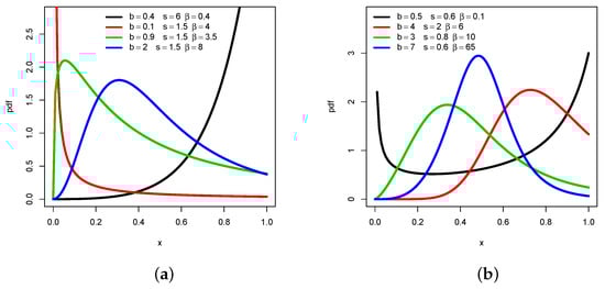
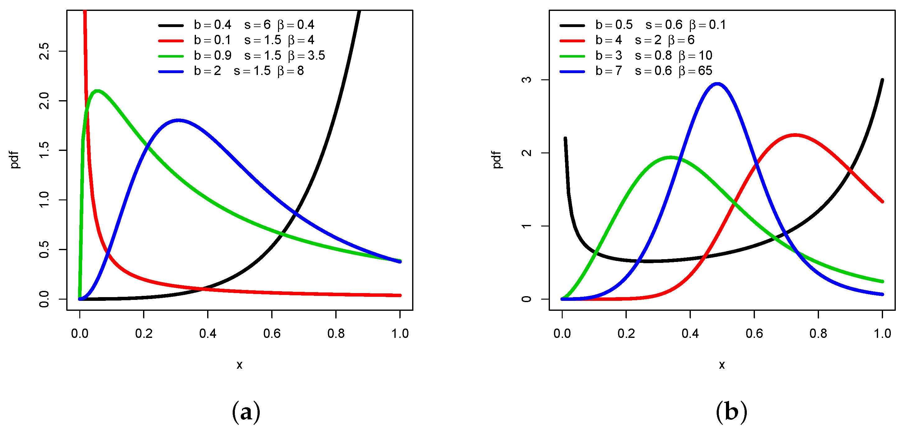
Figure 1. Plots of $f_{UG/G}(x;b,s,\beta )$ for several values of b, s and $\beta$ showing (a) decreasing, increasing, and “increasing-decreasing” highly right-skewed shapes, and (b) “increasing-decreasing” moderately right-skewed or almost symmetric and “decreasing-increasing” shapes.

From Figure 1a, the decreasing, increasing, and “increasing-decreasing” shapes of $f_{UG/G}(x;b,s,\beta )$ are observed, with the additional information that it can be skewed to the right in an abrupt manner. The green curve illustrates this last point. On the other hand, Figure 1b completes Figure 1a by showing “increasing-decreasing” with moderate right-skewed or almost symmetric shapes (see the blue line), and “decreasing-increasing” shapes. In particular, the black line is typical of what can be called a U shape. The wide variety of curvature possibilities possessed by this pdf is clearly a huge advantage of the UG/G distribution. It is useful in diverse statistical applications demanding a flexible distribution to capture all the information behind the data.

2.3. Survival and Hazard Rate Functions

It follows immediately from Equation (3) that the survival function (sf) of the UG/G distribution is given by $S_{UG/G}(x;b,s,\beta )=1-F_{UG/G}(x;b,s,\beta )$. That is

$$\begin{array}{c}\hfill S_{UG/G}(x;b,s,\beta )=\frac{{(1+(\beta -1)x^b)}^s-{\beta }^s{x}^{bs}}{{(1+(\beta -1)x^b)}^s},x\in (0,1),\end{array}$$

which can be completed with $S_{UG/G}(x;b,s,\beta )=1$ for $x\le 0$ and $S_{UG/G}(x;b,s,\beta )=0$ for $x\le 1$. The corresponding hrf is obtained quite standardly; it is given as $h_{UG/G}(x;b,s,\beta )=f_{UG/G}(x;b,s,\beta )/[1-F_{UG/G}(x;b,s,\beta )]$. That is

$$\begin{array}{c}\hfill h_{UG/G}(x;b,s,\beta )=\frac{bs{\beta }^s{x}^{bs-1}}{(1+(\beta -1)x^b)[{(1+(\beta -1)x^b)}^s-{\beta }^s{x}^{bs}]},x\in (0,1),\end{array}$$

and $h_{UG/G}(x;b,s,\beta )=0$ for $x\notin (0,1)$. Since they are informative in the modelling sense, some analytical properties of $h_{UG/G}(x;b,s,\beta )$ are now being examined. To begin, the following asymptotic properties hold:

$$\begin{array}{c}\hfill h_{UG/G}(x;b,s,\beta )\underset{x\to 0}{\sim }bs{\beta }^s{x}^{bs-1}=\left\{\begin{array}{cc}0\hfill & \mathrm{if}bs>1,\hfill \\ {\displaystyle {\beta }^s}\hfill & \mathrm{if}bs=1,\hfill \\ +\infty \hfill & \mathrm{if}bs\in (0,1),\hfill \end{array}\right.h_{UG/G}(x;b,s,\beta )\underset{x\to 1}{\sim }\frac{1}{1-x}=+\infty .\end{array}$$

For a fine analysis of the shape behavior of $h_{UG/G}(x;b,s,\beta )$, let us present the following function:

$$\begin{array}{cc}\hfill & {\left\{log\left[h_{UG/G}(x;b,s,\beta )\right]\right\}}^{\prime }=\hfill \\ \hfill & \frac{{\beta }^s[(b+1)(\beta -1)x^{b(s+1)}+x^{bs}]+(bs-1-(b+1)(\beta -1)x^b){(1+(\beta -1)x^b)}^s}{x(1+(\beta -1)x^b)[{(1+(\beta -1)x^b)}^s-{\beta }^s{x}^{bs}]}.\hfill \end{array}$$

This function is of high complexity, and its sign depends on some configurations of the parameters. As an immediate remark, we can notice that, for $\beta >1$ and $bs-1>(b+1)(\beta -1)$, then ${\left\{log\left[h_{UG/G}(x;b,s,\beta )\right]\right\}}^{\prime }\ge 0$, implying that $h_{UG/G}(x;b,s,\beta )$ is increasing. This result is completed with a graphical approach in Figure 2, demonstrating the capability of $h_{UG/G}(x;b,s,\beta )$ in terms of shapes.

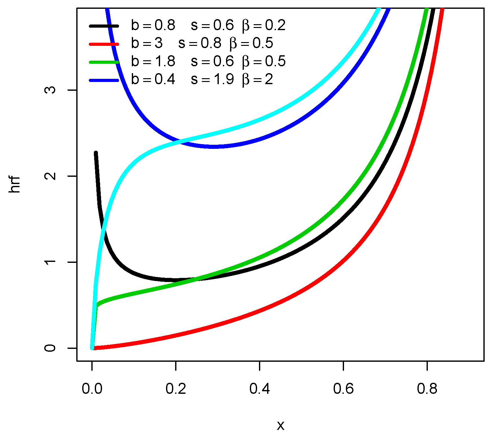
Figure 2. Plots of $h_{UG/G}(x;b,s,\beta )$ for several values of b, s, and $\beta$.

Hence, as shown in Figure 2, $h_{UG/G}(x;b,s,\beta )$ has a number of convex properties when it is increasing, and it can be “decreasing-increasing”. As a result, the U shape property is obtained for both the pdf and hrf of the UG/G distribution.

3. Relevant Properties

This section summarizes our most important results on the technical properties of the UG/G distribution.

3.1. Distributional Inequalities

The next result investigates some inequalities satisfied by the cdf of the UG/G distribution. These inequalities are the foundation of first order stochastic dominance (see [16]).

Proposition 2.

The function $F_{UG/G}(x;b,s,\beta )$ is

• decreasing with respect to the parameter b,
• decreasing with respect to the parameter s,
• increasing with respect to the parameter β.

Proof. 

Several ways of proof are possible. Here, we focus on the derivative approach.

• After several developments, we establish that

  $$\frac{\partial F_{UG/G}(x;b,s,\beta )}{\partial b}=\frac{s{\beta }^{s}log\left(x\right)x^{bs}}{{(1+(\beta -1)x^b)}^{s+1}}\le 0.$$
  Thus, the function $F_{UG/G}(x;b,s,\beta )$ is decreasing with respect to the parameter b.
• With the same approach, we have

  $$\frac{\partial F_{UG/G}(x;b,s,\beta )}{\partial s}=\frac{{\beta }^s{x}^{bs}\left[log\left(\beta \right)+blog\left(x\right)-log(1+(\beta -1)x^b)\right]}{{(1+(\beta -1)x^b)}^s}.$$
  Since

  $$log(1+(\beta -1)x^b)=log(1-x^b+\beta x^b)\ge log\left(\beta x^b\right)=log\left(\beta \right)+blog\left(x\right),$$

  we have $\partial F_{UG/G}(x;b,s,\beta )/\partial s\le 0$, and the function $F_{UG/G}(x;b,s,\beta )$ is decreasing with respect to the parameter s.
• Algebraic operations provide

  $$\frac{\partial F_{UG/G}(x;b,s,\beta )}{\partial \beta }=\frac{s{\beta }^{s-1}(1-x^b)x^{bs}}{{(1+(\beta -1)x^b)}^{s+1}}\ge 0.$$
  As a result, the function $F_{UG/G}(x;b,s,\beta )$ is increasing with respect to the parameter $\beta$. Proposition 2 is proven. □

Based on Proposition 2 and the remarks made in Equations (4) and (5), the following corollary involving the power and Marshall–Olkin extended power distributions is fulfilled.

Corollary 1.

The following first order stochastic order dominance results are valid.

• Let $\breve{F}(x;b,s)$ be the cdf of the power distribution, as defined in Equation (4). Then, for any $\beta \ge 1$, we have

  $$\breve{F}(x;b,s)\le F_{UG/G}(x;b,s,\beta ).$$
  The reversed inequality is satisfied for $\beta \in (0,1)$.
• Let $\dot{F}(x;b,\beta )$ be the cdf of the Marshall–Olkin extended power distribution as given in Equation (5). Then, for any $s\ge 1$, we have

  $$F_{UG/G}(x;b,s,\beta )\le \dot{F}(x;b,\beta ).$$
  The reversed inequality is satisfied for $s\in (0,1)$.

In comparison to the power and Marshall–Olkin extended power distributions, Corollary 1 shows how the UG/G distribution is placed in the stochastic sense. Based on the values of $\beta$ and s, we can see that the UG/G distribution achieves different modeling objectives. Further developments related to the first stochastic order can be found in [16].

3.2. Moment Properties

The raw moments of the UG/G distribution are the subject of the next proposition.

Proposition 3.

For any integer m, the mth moment of a random variable Y with the UG/G distribution is given as

$${\mu }_m^{\prime }=\mathbb{E}\left(Y^m\right)=\left\{\begin{array}{cc}{\displaystyle {\beta }^s\frac{sb}{m+sb}{}_2{F}_1\left(s+1,\frac{m}{b}+s;\frac{m}{b}+s+1;1-\beta \right)}\hfill & \mathrm{if}\beta \ne 1,\hfill \\ \\ {\displaystyle \frac{sb}{m+sb}}\hfill & x\in \mathrm{if}\beta =1,\hfill \end{array}\right.$$

where ${}_2{F}_1(a,b;c;z)$ denotes the Hypergeometric function defined by

$${}_2{F}_1(a,b;c;z)=\sum _{k=0}^{+\infty }\frac{{\left(a\right)}_k{\left(b\right)}_k}{{\left(c\right)}_k}\frac{z^k}{k!},{\left(q\right)}_k=\left\{\begin{array}{cc}1\hfill & k=0,\hfill \\ q(q+1)\cdots (q+k-1)\hfill & k>0.\hfill \end{array}\right.$$

Proof. 

Let X be a random variable with the G/G distribution. Then, the moment generating function of X is given by $M\left(t\right)=\mathbb{E}\left(e^{-tX}\right)$, and it is expressed in [11]. Since the distribution of Y is the one of $e^{-X}$, by remarking that ${\mu }_m^{\prime }=\mathbb{E}\left(Y^m\right)=\mathbb{E}\left(e^{-mX}\right)=M\left(m\right)$, the desired expressions comes by taking $t=m$ into $M\left(t\right)$. The proof of Proposition 3 ends. □

Based on Proposition 3, we can calculate the mean of Y given by ${\mu }_1^{\prime }=\mathbb{E}\left(Y\right)$ and variance of Y given by ${\sigma }^2=E\left({(Y-{\mu }_1^{\prime })}^2\right)={\mu }_2^{\prime }-{\left({\mu }_1^{\prime }\right)}^2$. The standard deviation $\sigma$ follows immediately by taking the square root. The moments skewness of Y is obtained by

$$S=\frac{1}{{\sigma }^3}\mathbb{E}\left[{(Y-{\mu }_1^{\prime })}^3\right]$$

and the moment kurtosis of Y can be expressed as

$$K=\frac{1}{{\sigma }^4}\mathbb{E}\left[{(Y-{\mu }_1^{\prime })}^4\right].$$

We can expand the expressions of these measures by applying the standard binomial formula. Table 1 displays some numerical values of the aforementioned moment measures. The considered values of the parameters are picked haphazardly in order to demonstrate the adaptability of the above-moment measures.

Table 1. The values of some moment measures for the UG/G distribution for several values of b, s, and $\beta$.

$(\mathit{b},\mathit{s},\mathit{\beta })$	${\mathit{\mu }}_1^{\prime }$	${\mathit{\mu }}_2^{\prime }$	${\mathit{\mu }}_3^{\prime }$	${\mathit{\mu }}_4^{\prime }$	${\mathit{\sigma }}^2$	S	K
$(0.1,0.5,0.5)$	0.0848	0.0457	0.0313	0.0238	0.0385	2.7683	10.1353
$(0.1,0.5,2)$	0.0255	0.0126	0.0083	0.0062	0.0119	5.6826	38.0804
$(0.1,0.5,4)$	0.0132	0.0064	0.0042	0.0031	0.0062	8.0598	75.1552
$(2,0.5,4)$	0.0387	0.0190	0.1111	0.0798	0.0624	0.7445	2.6686
$(0.1,1.5,4)$	0.3333	0.1735	0.0126	0.0094	0.0175	4.5246	24.7938
$(2,2,2)$	0.7123	0.5451	0.4380	0.3644	0.0376	-0.5479	2.5365
$(2,2,5)$	0.5786	0.3823	0.2766	0.2132	0.0474	0.0383	2.0981
$(5,0.5,0.5)$	0.7699	0.6349	0.5446	0.4791	0.0421	-1.0558	3.3949
$(7,0.6,17)$	0.5966	0.3824	0.2598	0.1853	0.0265	0.0043	2.7365
$(7,0.6,10)$	0.6370	0.4337	0.3110	0.2327	0.0278	-0.1572	2.6743

From Table 1, we observe that the UG/G distribution can be left and right skewed due to some negative and positive values for S. Furthermore, the UG/G distribution encompasses all kurtosis states; when we compare K to 3, which is the value of reference for a kurtosis associated to a standard normal distribution, we can see that it can be lower, nearly equal, or greater. The observations presented in Figure 1 substantiate these findings.

3.3. Quantile Properties

The quantile function (qf) of the UG/G distribution is given as $Q_{UG/G}(y;b,s,\beta )=F_{UG/G}^{-1}(y;b,s,\beta )$, $y\in (0,1)$. That is, after some elementary operations, we obtain

$$\begin{array}{c}\hfill Q_{UG/G}(y;b,s,\beta )={\left(1+\beta (y^{-1/s}-1)\right)}^{-1/b}.\end{array}$$

(6)

The concept of qf has been used in a number of academic and practical publications. Several measures of position, skewness, and kurtosis can be defined based on this function. For example, the median of the UG/G distribution is just the second main quartile, which may be written as

$$Q_2=Q_{UG/G}\left(\frac{1}{2};b,s,\beta \right)={\left(1+\beta (2^{1/s}-1)\right)}^{-1/b}.$$

As useful quantile skewness measure, we can mention the Bowley skewness expressed as

$$S_B=\frac{Q_3-2Q_2+Q_1}{IR},$$

where $Q_i$ denotes the ith quartile of the UG/G distribution, i.e., $Q_i=Q_{UG/G}(i/4;b,s,\beta )$, and $IR=Q_3-Q_1$. Furthermore, as a famous quantile kurtosis measure, the Moors kurtosis is defined by

$$K_M=\frac{O_7-O_5-O_3+O_1}{IR},$$

where $O_i$ denotes the ith octile of the UG/G distribution, i.e., $O_j=Q_{UG/G}(j/8;b,s,\beta )$, $j=1,2,3$, and 4. Finally, we can create values from the UG/G distribution by taking advantage of the fact that $Q_{UG/G}(Z;b,s,\beta )$ has the UG/G distribution for any random variable Z with the unit uniform distribution. To put it another way, the qf converts values from the unit uniform distribution to values from the UG/G distribution. The book of [17] contains more material on the issue of quantile analysis.

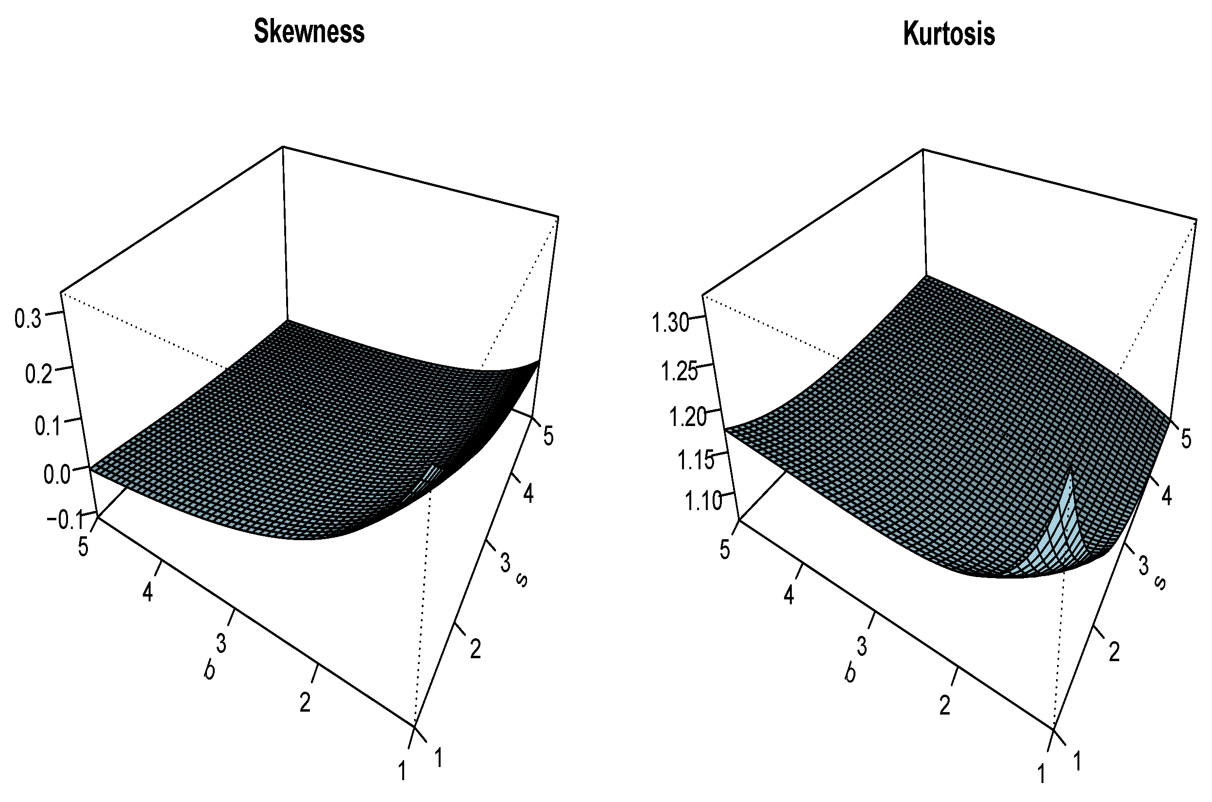
Figure 3 and Figure 4 complete the quantile study above by presenting three-dimensional plots of the Bowley skewness and Moors kurtosis of the UG/G distribution for several values of b, s, and $\beta$.

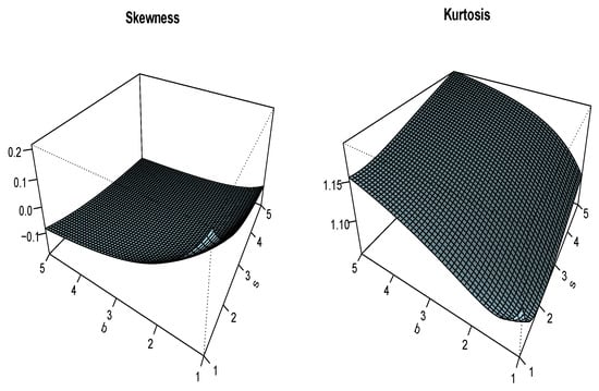
Figure 3. Plots of the Bowley skewness and Moors kurtosis of the UG/G distribution for $(b,s)\in {[1,5]}^2$ and $\beta =2.5$.

Figure 4. Plots of the Bowley skewness and Moors kurtosis of the UG/G distribution for $(b,s)\in {[1,5]}^2$ and $\beta =5$.

From Figure 3 and Figure 4, we see that the Bowley skewness can be negative or positive, indicating left or right skewed properties of the UG/G distribution, already evoked via the moment skewness. In addition, the kurtosis is discovered to be non-monotonic, with values ranging from small to large.

3.4. Reliability Coefficient

The strength loss and system collapse strategies are prevalent in many physical systems. It is vital to consider valuable measures of reliability when evaluating them. This is especially true when a component of a system is subjected to random stress and random strength. The chance that stress surpasses strength is critical. In this scenario, we can describe the stress with a random variable $X_2$ and the stress with a random variable $X_1$. Then, $\mathfrak{R}=\mathbb{P}(X_2\le X_1)$ can be used to calculate the chances that the stress surpasses the strength. Further modeling and detail on this coefficient can be found in [18]. In the following result, we determine $\mathfrak{R}$ in a special distributional configuration involving the UG/G distribution.

Theorem 1.

Let $Y_1$ and $Y_2$ be two independent random variables with the UG/G distribution with parameters $(b,s_1,\beta )$ and $(b,s_2,\beta )$, respectively. Then, we have

$$\begin{array}{cc}\hfill \mathfrak{R}& =\mathbb{P}(Y_2\le Y_1)=\frac{s_1}{s_1+s_2}.\hfill \end{array}$$

Proof. 

The proof is primarily mathematical; we have

$$\begin{array}{cc}\hfill \mathfrak{R}& =\mathbb{P}(Y_2\le Y_1)={\int }_{-\infty }^{+\infty }{F}_{UG/G}(x;b,s_2,\beta )f_{UG/G}(x;b,s_1,\beta )dx\hfill \\ \hfill & ={\int }_0^1\frac{{\beta }^{s_2}{x}^{b{s}_2}}{{(1+(\beta -1)x^b)}^{s_2}}\frac{b{s}_1{\beta }^{s_1}{x}^{b{s}_1-1}}{{(1+(\beta -1)x^b)}^{s_1+1}}dx\hfill \\ \hfill & ={\int }_0^1\frac{b{s}_1{\beta }^{s_1+s_2}{x}^{b(s_1+s_2)-1}}{{(1+(\beta -1)x^b)}^{s_1+s_2+1}}dx=\frac{s_1}{s_1+s_2}{\int }_0^1{f}_{UG/G}(x;b,s_1+s_2,\beta )dx\hfill \\ \hfill & =\frac{s_1}{s_1+s_2}.\hfill \end{array}$$

The right result is accomplished. □

The analysis of the stress-strength UG/G model is possible using Theorem 1. Thanks to the simple form of $\mathfrak{R}$, which only depends on $s_1$ and $s_2$, the substitution approach can be used to estimate it. It is worth noting that, when $Y_1$ and $Y_2$ are identically distributed, we get $\mathfrak{R}=1/2$, which is the expected value, whatever the assumptions made on the common distribution.

4. Estimation with Simulation

A parameter estimation strategy is now being developed for the proposed unit distribution.

4.1. Estimation

Let $y_1,\dots ,y_n$ be n positive values that are expected to be observed from a random variable with the UG/G distribution in which the parameters b, s, and $\beta$ are supposed to be unknown. In particular, by nature, we have $y_i\in (0,1)$ for any $i=1,\dots ,n$. Then, the log-likelihood function related to b, s and $\beta$ is defined by

$$\begin{array}{cc}\hfill & \mathfrak{L}(b,s,\beta )=\sum _{i=1}^{n}log\left[f_{UG/G}(y_i;b,s,\beta )\right]\hfill \\ \hfill & =nlog\left(b\right)+nlog\left(s\right)+nslog\left(\beta \right)+(bs-1)\sum _{i=1}^{n}log\left(y_i\right)-(s+1)\sum _{i=1}^{n}log(1+(\beta -1)y_i^b).\hfill \end{array}$$

The maximum likelihood estimates (MLEs) of b, s, and $\beta$ depending only on $y_1,\dots ,y_n$, can be defined as $\widehat{b}$, $\widehat{s}$, and $\widehat{\beta }$, where $(\widehat{b},\widehat{s},\widehat{\beta })=argmax\mathfrak{L}(b,s,\beta )$. The maximization is taken over the possible values of the parameters. These MLEs also satisfy the following partial derivative equations: $\partial \mathfrak{L}(b,s,\beta )/\partial b=0$, $\partial \mathfrak{L}(b,s,\beta )/\partial s=0$, and $\partial \mathfrak{L}(b,s,\beta )/\partial \beta =0$, where

$$\begin{array}{c}\hfill \frac{\partial \mathfrak{L}(b,s,\beta )}{\partial b}=\frac{n}{b}+s\sum _{i=1}^{n}log\left(y_i\right)-(s+1)(\beta -1)\sum _{i=1}^n\frac{y_i^{b}log\left(y_i\right)}{1+(\beta -1)y_i^b},\end{array}$$

$$\begin{array}{c}\hfill \frac{\partial \mathfrak{L}(b,s,\beta )}{\partial s}=\frac{n}{s}+nlog\left(\beta \right)+b\sum _{i=1}^{n}log\left(y_i\right)-\sum _{i=1}^{n}log(1+(\beta -1)y_i^b)\end{array}$$

and

$$\begin{array}{c}\hfill \frac{\partial \mathfrak{L}(b,s,\beta )}{\partial \beta }=\frac{ns}{\beta }-(s+1)\sum _{i=1}^n\frac{y_i^b}{1+(\beta -1)y_i^b}.\end{array}$$

Due to the complexity of these partial derivatives, there are few opportunities to find closed-form expressions for $\widehat{b}$, $\widehat{s}$, and $\widehat{\beta }$. To discover accurate numerical solutions, numerical approaches such as the (quasi) Newton–Raphson method can be utilized.

Using $\widehat{b}$, $\widehat{s}$, and $\widehat{\beta }$, we can estimate the pdf of the UG/G distribution by the substitution method; we can consider $\widehat{f}\left(x\right)=f_{UG/G}(x;\widehat{b},\widehat{s},\widehat{\beta })$ as a pertinent functional estimate of $f_{UG/G}(x;b,s,\beta )$. The same method can be applied to estimate the cdf, hrf, and so on.

The theory underlying the MLEs is well-known and can be applied in the setting of the UG/G distribution without any problem. In particular, the asymptotic distribution of the random version of $(\widehat{b},\widehat{s},\widehat{\beta })$ can be identified by a three-dimensional normal distribution with the mean $(b,s,\beta )$ and matrix of covariance: $\mathfrak{C}=I{(b,s,\beta )}^{-1}{\mid }_{(b,s,\beta )=(\widehat{b},\widehat{s},\widehat{\beta })}$, where $I(b,s,\beta )$ denotes the following symmetric matrix:

$$\begin{array}{c}\hfill I(b,s,\beta )=-\left(\begin{array}{ccc}\frac{{\partial }^2\mathfrak{L}(b,s,\beta )}{\partial b^2}& \frac{{\partial }^2\mathfrak{L}(b,s,\beta )}{\partial b\partial s}& \frac{{\partial }^2\mathfrak{L}(b,s,\beta )}{\partial b\partial \beta }\\ .& \frac{{\partial }^2\mathfrak{L}(b,s,\beta )}{\partial s^2}& \frac{{\partial }^2\mathfrak{L}(b,s,\beta )}{\partial s\partial \beta }\\ .& .& \frac{{\partial }^2\mathfrak{L}(b,s,\beta )}{\partial {\beta }^2}\end{array}\right).\end{array}$$

(7)

The components in $I(b,s,\beta )$ can be found in the Appendix A. The matrix $\mathfrak{C}$ can be numerically calculated using mathematical tools. Based on the obtained three-dimentional normal distribution, we can define approximate confidence intervals (CIs) for b, s, and $\beta$ at a given level, say $100(1-p)\%$ with $p\in (0,1)$. The formulas for the related lower bounds (CI-Ls) and upper bounds (CI-Us) of such intervals remain conventional; if we focus on the unknown parameter $\alpha$, these bounds are given by CI-L $=\widehat{\alpha }-z_p{\mathrm{SE}}_{\alpha }$ and CI-U $=\widehat{\alpha }+z_p{\mathrm{SE}}_{\alpha }$, where $z_p$ is defined by $\mathbb{P}\left(\right|Z|\ge z_p)=p$, where Z denotes a random variable with the standard normal distribution, and ${\mathrm{SE}}_{\alpha }$ refers to the standard error (SE) of $\widehat{\alpha }$, defined by the square root of the element of the diagonal of the matrix of covariance $\mathfrak{C}$ located at the same position of $\alpha$ in the unknown vector $(b,s,\beta )$. The technical developments behind the MLEs can be found in [19].

4.2. Simulation

In the sequel, we illustrate and provide simulation results to evaluate the behavior of the obtained MLEs. In this case, we use the R software developed by [20]. The following process is considered:

• We generate 5000 random samples of the form $(y_1,\dots ,y_n)$ from the UG/G distribution, where, using Equation (6), $y_i$ is calculated by the following formula:

  $$y_i=Q_{UG/G}(z_i;b,s,\beta )={\left(1+\beta (z_i^{-1/s}-1)\right)}^{-1/b},$$

  where $(z_1,\dots ,z_n)$ denotes a sample of values generated from the uniform distribution over $(0,1)$.
• Different sample sizes are considered as $n=100$, 200, 300, and 1000.
• Five different configurations for the vector of parameters $(b,s,\beta )$ are chosen as Config1: $(0.5,0.5,0.5)$, Config2: $(0.8,0.5,0.5)$, Config3: $(1.2,0.5,0.5)$, Config4: $(0.5,1.5,0.5)$, and Config5: $(0.8,0.8,0.8)$.
• The average MLEs, mean square errors (MSEs), CI-Ls, CI-Us, and lengths (LENs) of the CIs with two different levels (90% and 95%) for the considered configurations are calculated.
• The obtained results are mentioned in Table 2, Table 3, Table 4, Table 5 and Table 6, for Config1, Config2, Config3, Config4, and Config5, respectively.
  Table 2. Numerical values of the MLEs, MSEs, CI-Ls, CI-Us, and LENs for the parameters of the UG/G model for Config1.

  n	MLE	MSE	90%			95%
  			CI-L	CI-U	LEN	CI-L	CI-U	LEN
  100	0.7832	0.3237	−0.9990	2.5653	3.5643	−1.3402	2.9066	4.2468
  	0.4658	0.1469	−0.6565	1.5882	2.2448	−0.8715	1.8032	2.6746
  	0.5403	0.0217	0.2304	0.7703	0.5398	0.1787	0.8219	0.6432
  200	0.7412	0.3025	−0.1981	1.6806	1.8787	−0.3780	1.8604	2.2385
  	0.5391	0.1328	−0.2259	1.3078	1.5337	−0.3728	1.4546	1.8274
  	0.5205	0.0211	0.2944	0.7466	0.4522	0.2511	0.7899	0.5388
  300	0.5968	0.2014	−0.0601	1.2537	1.3138	−0.1859	1.3795	1.5654
  	0.5384	0.1249	−0.0273	1.2240	1.2513	−0.1471	1.3438	1.4909
  	0.4499	0.0075	0.2783	0.6215	0.3432	0.2455	0.6544	0.4089
  1000	0.5546	0.0816	0.2020	0.9071	0.7051	0.1345	0.9746	0.8401
  	0.5346	0.0429	0.2309	0.8383	0.6074	0.1727	0.8964	0.7237
  	0.4994	0.0019	0.3817	0.5571	0.1754	0.3649	0.5739	0.2090

  Table 3. Numerical values of the MLEs, MSEs, CI-Ls, CI-Us, and LENs for the parameters of the UG/G model for Config2.

  n	MLE	MSE	90%			95%
  			CI-L	CI-U	LEN	CI-L	CI-U	LEN
  100	1.1549	1.2964	−2.3567	3.9877	6.3444	−2.9641	4.5951	7.5592
  	0.7710	0.3566	−0.9496	2.4915	3.4412	−1.2791	2.8210	4.1001
  	0.5225	0.0436	0.1247	0.9204	0.7957	0.0485	0.9966	0.9481
  200	1.1095	0.5145	−0.4835	2.7025	3.1860	−0.7886	3.0075	3.7961
  	0.5361	0.1180	−1.0089	2.0811	3.0900	−1.3047	2.3770	3.6817
  	0.4940	0.0277	0.2668	0.7212	0.4544	0.2233	0.7647	0.5414
  300	0.8494	0.3305	−0.1723	1.8712	2.0435	−0.3680	2.0668	2.4348
  	0.5151	0.0326	−0.0309	1.0612	1.0921	−0.1355	1.1657	1.3012
  	0.4943	0.0100	0.3269	0.6576	0.3306	0.2953	0.6892	0.3940
  1000	0.8046	0.2140	0.2557	1.7452	1.4896	0.1131	1.8879	1.7748
  	0.4977	0.0197	0.1769	0.7186	0.5417	0.1250	0.7705	0.6455
  	0.4958	0.0045	0.4014	0.5862	0.1848	0.3837	0.6039	0.2202

  Table 4. Numerical values of the MLEs, MSEs, CI-Ls, CI-Us, and LENs for the parameters of the UG/G model for Config3.

  n	MLE	MSE	90%			95%
  			CI-L	CI-U	LEN	CI-L	CI-U	LEN
  100	1.5224	1.5864	−3.0280	6.0727	9.1008	−3.8994	6.9441	10.8435
  	0.7189	0.2086	−2.3250	3.7628	6.0878	−2.9079	4.3457	7.2535
  	0.6220	0.1336	0.2395	1.0045	0.7650	0.1663	1.0778	0.9115
  200	1.3579	0.3145	−1.5575	4.0732	5.6308	−2.0967	4.6124	6.7090
  	0.5978	0.1984	−0.6051	1.8007	2.4058	−0.8354	2.0311	2.8665
  	0.5621	0.0271	0.3071	0.7772	0.4701	0.2621	0.8222	0.5601
  300	1.2796	0.2757	−0.1065	2.2656	2.3721	−0.3336	2.4927	2.8263
  	0.5868	0.1783	−0.0473	1.4209	1.4682	−0.1879	1.5614	1.7493
  	0.4577	0.0081	0.2770	0.6184	0.3414	0.2443	0.6511	0.4068
  1000	1.2109	0.0939	0.4768	2.1450	1.6682	0.3171	2.3047	1.9876
  	0.4746	0.0091	0.2083	0.7409	0.5327	0.1573	0.7919	0.6347
  	0.4833	0.0042	0.3975	0.5690	0.1714	0.3811	0.5854	0.2043

  Table 5. Numerical values of the MLEs, MSEs, CI-Ls, CI-Us, and LENs for the parameters of the UG/G model for Config4.

  n	MLE	MSE	90%			95%
  			CI-L	CI-U	LEN	CI-L	CI-U	LEN
  100	0.8165	0.3955	−1.8587	3.4916	5.3503	−2.3709	4.0039	6.3748
  	1.3397	0.7860	−2.2552	4.9347	7.1899	−2.9436	5.6231	8.5667
  	0.6501	0.1530	0.1890	1.1113	0.9223	0.1007	1.1996	1.0989
  200	0.5776	0.1843	−1.3949	2.5502	3.9451	−1.7726	2.9279	4.7005
  	1.5248	0.5228	−1.3644	4.4140	5.7784	−1.9177	4.9672	6.8849
  	0.6354	0.1158	0.2678	1.0393	0.7715	0.1939	1.1132	0.9193
  300	0.4614	0.0988	−0.3973	1.3200	1.7173	−0.5617	1.4844	2.0461
  	1.5144	0.4258	−0.5995	3.6084	4.2079	−1.0024	4.0113	5.0137
  	0.5331	0.0220	0.2356	0.8305	0.5949	0.1787	0.8875	0.7088
  1000	0.4969	0.0553	−0.0350	1.0288	1.0637	−0.1368	1.1306	1.2674
  	1.9444	0.4116	0.1399	2.7490	2.6092	−0.1100	2.9988	3.1088
  	0.4988	0.0064	0.3230	0.6745	0.3515	0.2894	0.7082	0.4189

  Table 6. Numerical values of the MLEs, MSEs, CI-Ls, CI-Us, and LENs for the parameters of the UG/G model for Config5.

  n	MLE	MSE	90%			95%
  			CI-L	CI-U	LEN	CI-L	CI-U	LEN
  100	0.7018	0.4537	−2.8842	4.2877	7.1718	−3.5708	4.9744	8.5452
  	1.1850	0.9061	−2.9198	5.2898	8.2096	−3.7058	6.0758	9.7816
  	0.6178	0.1673	0.0955	1.1400	1.0445	−0.0045	1.2401	1.2446
  200	0.8635	0.3419	−1.3834	3.1103	4.4937	−1.8136	3.5406	5.3542
  	1.1541	0.7736	−2.2933	4.6016	6.8949	−2.9535	5.2617	8.2152
  	0.8574	0.1217	0.4107	1.3042	0.8935	0.3251	1.3898	1.0646
  300	0.8141	0.1459	−1.2982	2.7264	4.0246	−1.6835	3.1118	4.7953
  	0.9337	0.0750	−1.3201	3.1875	4.5076	−1.7517	3.6191	5.3708
  	0.8273	0.0384	0.5016	1.1129	0.6113	0.4431	1.1715	0.7284
  1000	0.8061	0.0843	−1.0367	2.7688	3.8055	−1.4011	3.1332	4.5343
  	0.8196	0.0463	−0.9275	2.5667	3.4942	−1.2621	2.9012	4.1633
  	0.8184	0.0133	0.6501	1.0066	0.3565	0.6160	1.0408	0.4248

We can see from these tables that, when n increases, the values of MLEs are close to the values of the parameters specified in the configurations. Moreover, when n increases, the values of the MSEs and LENs decrease as expected.

5. Applications

In this section, we use two real data sets to demonstrate the accuracy of the UG/G model. In the first example, we look at trade share data, and in the second, we look at flood level data.

5.1. Application 1

The first data set, named as the trade share data set, considers the values of the variable trade share involved in the famous “Determinants of Economic Growth Data". The growth rates of up to 61 countries, along with variables that are potentially related to growth, are taken. The data are freely available as an online complement to [21]. Numerically, the following values constitute the trade share data set: 0.140501976, 0.156622976, 0.157703221, 0.160405084, 0.160815045, 0.22145839, 0.299405932, 0.31307286, 0.324612707, 0.324745566, 0.329479247, 0.330021679, 0.337879002, 0.339706242, 0.352317631, 0.358856708, 0.393250912, 0.41760394, 0.425837249, 0.43557933, 0.442142904, 0.444374621, 0.450546652, 0.4557693, 0.46834656, 0.473254889, 0.484600782, 0.488949597, 0.509590268, 0.517664552, 0.527773321, 0.534684658, 0.543337107, 0.544243515, 0.550812602, 0.552722335, 0.56064254, 0.56074965, 0.567130983, 0.575274825, 0.582814276, 0.603035331, 0.605031252, 0.613616884, 0.626079738, 0.639484167, 0.646913528, 0.651203632, 0.681555152, 0.699432909, 0.704819918, 0.729232311, 0.742971599, 0.745497823, 0.779847085, 0.798375845, 0.814710021, 0.822956383, 0.830238342, 0.834204197, and 0.979355395.

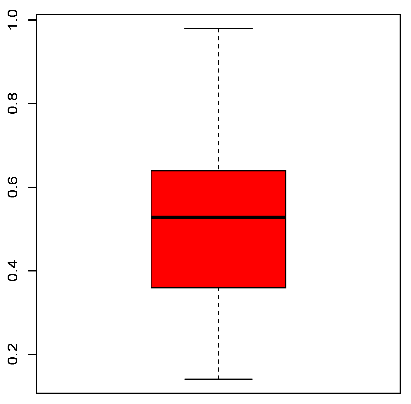
Figure 5 shows the quantile characteristics of the trade share data set via a boxplot.

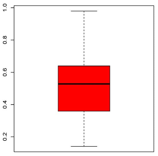
Figure 5. Boxplot for the trade share data set.

From Figure 5, we see that the data are rather right-skewed and almost symmetrical. There is no atypical value. Table 7 completes this basic analysis by showing the statistical summary.

Table 7. Statistical summary for the trade share data set.

n	Mean	Median	Standard Deviation	Skewness	Kurtosis	Min	Max
61	0.5141	0.5277	0.1935	0.0260	2.5525	0.1405	0.9793

From Table 7, we can say that the trade share data are right-skewed and platykurtic or near platykurtic with a moderate standard deviation.

As a main statistical work, we analyze this data set via a fitting approach. In this regard, we compare the fit of the proposed UG/G model and those of the Kumaraswamy (Kw), beta (Beta), UR (recalling that it refers to the unit Rayleigh distribution by [10]), Topp-Leone (Topp), power (Power), and Transmuted (TM) models. These competitive models are defined by specific cdfs, which are recalled below.

• Kw distribution:

  $$F_{Kw}(x;\alpha ,\beta )=1-{(1-x^{\alpha })}^{\beta },x\in (0,1),$$
  $F_{Kw}(x;\alpha ,\beta )=0$ for $x\le 0$, and $F_{Kw}(x;\alpha ,\beta )=1$ for $x\ge 1$, with $\alpha ,\beta >0$.
• Beta distribution:

  $$F_{Beta}(x;\alpha ,\beta )=\frac{1}{B(\alpha ,\beta )}{\int }_0^x{t}^{\alpha -1}{(1-t)}^{\beta -1}dt,x\in (0,1),$$

  with $B(\alpha ,\beta )={\int }_0^1{t}^{\alpha -1}{(1-t)}^{\beta -1}dt$, $F_{Beta}(x;\alpha ,\beta )=0$ for $x\le 0$, and $F_{Beta}(x;\alpha ,\beta )=1$ for $x\ge 1$, with $\alpha ,\beta >0$.
• UR distribution:

  $$F_{UR}(x;\beta )=e^{-\beta {(log\left(x\right))}^2},x\in (0,1),$$
  $F_{UR}(x;\beta )=0$ for $x\le 0$, and $F_{UR}(x;\beta )=1$ for $x\ge 1$, with $\beta >0$.
• Topp distribution:

  $$F_{Topp}(x;\gamma )=x^{\gamma }{(2-x)}^{\gamma },x\in (0,1),$$
  $F_{Topp}(x;\gamma )=0$ for $x\le 0$, and $F_{Topp}(x;\gamma )=1$ for $x\ge 1$, with $\gamma >0$.
• Power distribution:

  $$F_{Power}(x;\beta )=x^{\beta },x\in (0,1),$$
  $F_{Power}(x;\beta )=0$ for $x\le 0$, and $F_{Power}(x;\beta )=1$ for $x\ge 1$, with $\beta >0$.
• TM distribution:

  $$F_{TM}(x;\lambda )=(1+\lambda )x-\lambda x^2,x\in (0,1),$$
  $F_{TM}(x;\lambda )=0$ for $x\le 0$, and $F_{TM}(x;\lambda )=1$ for $x\ge 1$, with $\lambda \in [-1,1]$.

Table 8 shows the MLEs of the model parameters, together with their SEs.

Table 8. Estimates (MLEs and SEs under parentheses) associated to the model parameters for the trade share data set.

Model	Estimates
UG/G	6.8537	0.3533	15.1067
$(b,s,\beta )$	(2.6613)	(0.1853)	(0.1043)
Kw	2.3296	2.7629	-
$(\alpha ,\beta )$	(0.3055)	(0.5550)	-
Beta	2.7943	2.6041	-
$(\alpha ,\beta )$	(0.4880)	(0.4519)	-
UR	1.2995	-	-
$\left(\beta \right)$	(0.1663)	-	-
Topp	2.7391	-	-
$\left(\gamma \right)$	(0.3507)	-	-
Power	1.3288	-	-
$\left(\beta \right)$	(0.1701)	-	-
TM	−0.1917	-	-
$\left(\lambda \right)$	(0.3313)	-	-

In order to compare fitted models, we employ the classic AIC, W, A, KS, KS (p-value) measures, which correspond to the Akaike, Anderson-Darling, Kolmogorov–Smirnov measures, with the p-value relating to the Kolmogorov–Smirnov test, respectively. Table 9 contains their values for the trade share data set and the considered models.

Table 9. AIC, W, A, KS, and KS (p-value) values for the trade share data set.

Model	AIC	W	A	KS	KS (p-Value)
UG/G	−24.4739	0.0243	0.2392	0.0507	0.9953
Kw	−23.2502	0.0526	0.4005	0.0689	0.9142
Beta	−23.9120	0.0490	0.3864	0.0617	0.9629
UR	−24.1938	0.0769	0.6082	0.0963	0.5892
Topp	−23.9794	0.0458	0.3740	0.0859	0.7258
Power	−2.4955	0.0495	0.3912	0.2213	0.0041
TM	1.6683	0.0527	0.4046	0.1792	0.0347

According to Table 9, the UG/G model has the smallest values for the AIC, W, A, KS measures, and the largest value for the KS (p-value), which is equal to $0.9953$, so nearly equal to 1. As a result of these criteria and the trade share data set, we can declare that it is the best fit among the models studied.

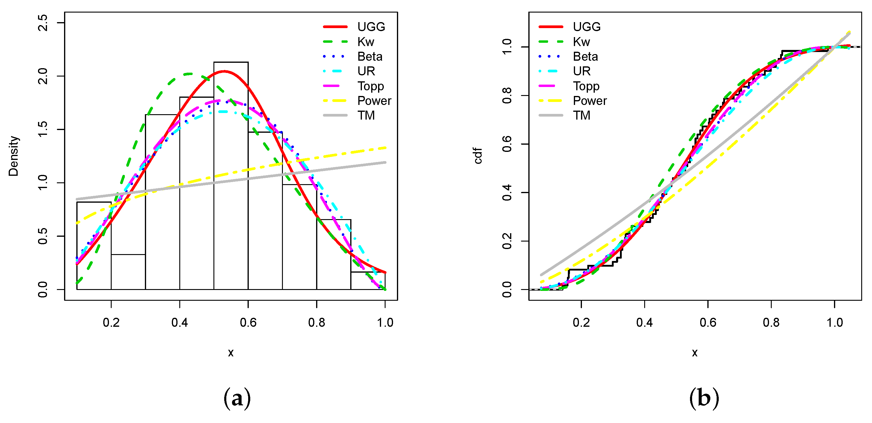
This superiority in fitting is visualized in Figure 6.

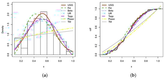
Figure 6. Plots of the (a) estimated pdfs and (b) estimated cdfs of the considered models and the trade share data set.

From Figure 6, we see that the fits of the estimated pdf and cdf of the UG/G model are the best. In particular, the estimated pdf shapes the global form of the histogram well. Furthermore, the top of the histogram has been captured well. The estimated UG/G model contains most of the information underlying the data.

5.2. Application 2

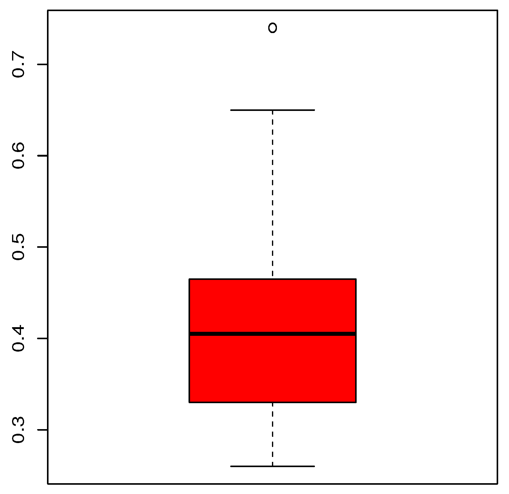
The second data set is extracted from [22] and refers to 20 observations of the Susquehanna River’s maximum flood level located at Harrisburg, Pennsylvania. The unit is a million cubic feet per second. The precise values are: 0.26, 0.27, 0.30, 0.32, 0.32, 0.34, 0.38, 0.38, 0.39, 0.40, 0.41, 0.42, 0.42, 0.42, 0.45, 0.48, 0.49, 0.61, 0.65, and 0.74.

These data are analyzed using the same methodology as in the previous application. To begin, Figure 7 depicts the elementary statistical properties of the flood level data set using a boxplot.

Figure 7. Boxplot for the flood level data set.

From Figure 7, we see that the data are rather right-skewed. One atypical value is identified; it is $0.74$, but its presence in the data set remains justified in practice. The statistical summary for the flood level data set is shown in Table 10.

Table 10. Statistical summary for the flood level data set.

n	Mean	Median	Standard Deviation	Skewness	Kurtosis	Min	Max
20	0.4225	0.4050	0.1244	1.0734	3.6624	0.26	0.74

The parameter estimates, as well as their related SEs, are shown in Table 11.

Table 11. Estimates (MLEs and SEs under parentheses) associated to the model parameters for the flood level data set.

Model	Estimates
UG/G	4.4987	7.1872	239.2606
$(b,s,\beta )$	(1.4263)	(3.4150)	(2.6653)
Kw	3.3773	12.0018
$(\alpha ,\beta )$	(0.6041)	(5.4713)
Beta	6.8309	9.2364
$(\alpha ,\beta )$	(2.1179)	(2.8912)
UR	1.1366
$\left(\beta \right)$	(0.2541)
Topp	2.2412
$\left(\gamma \right)$	(0.5011)
Power	1.7804
$\left(\beta \right)$	(0.2487)

Table 12 shows the values for the AIC, W, A, KS, and KS (p-value) of the flood level data set and the considered models.

Table 12. AIC, W, A, KS, and KS (p-value) values for the flood level data set.

Model	AIC	W	A	KS	KS (p-Value)
UG/G	−26.4875	0.0442	0.2610	0.1416	0.8168
Kw	−21.9465	0.1672	0.9746	0.2175	0.3004
Beta	−24.3671	0.1267	0.7514	0.2062	0.3625
UR	−20.2352	0.0892	0.5367	0.2892	0.0704
Topp	−12.7627	0.1194	0.7110	0.3409	0.0191
Power	1.7804	0.1229	0.7300	0.3977	0.0035

According to Table 12, the UG/G model has the smallest values for the AIC, W, A, and KS measures and the largest value for the KS (p-value), which is equal to $0.8168$. As a result of these facts, we may conclude that it has the best fit of all the models studied. It is worth mentioning that the TM model was left out of the competition due to its poor fit.

This superiority in fitting is visualized in Figure 6.

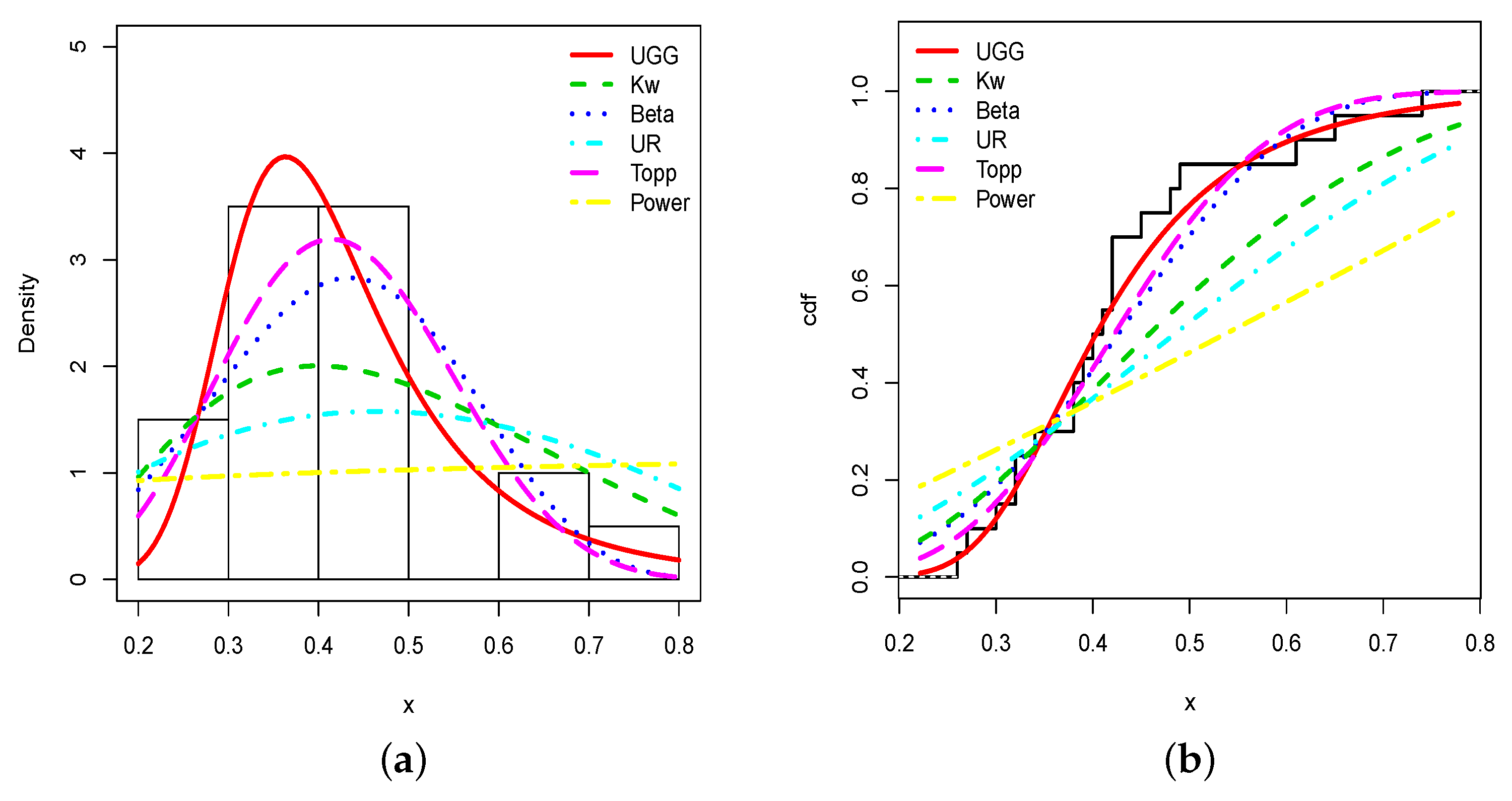
The estimated pdf and cdf fits of the UG/G model are the best, as shown in Figure 8. The estimated pdf, in particular, determines the overall shape of the histogram, as well as a nice capture of the top of the histogram and its right skewed portion.

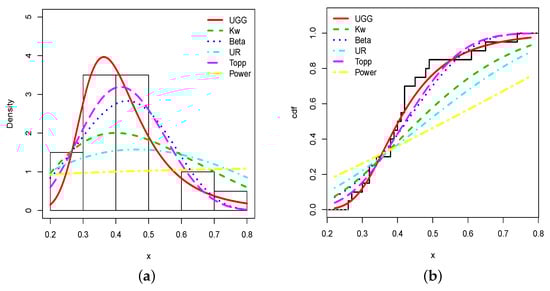
Figure 8. Plots of the (a) estimated pdfs and (b) estimated cdfs of the considered models and the flood level data set.

5.3. Complementary Analysis

Here, we provide some complementary analysis to the trade share and flood level data sets via the UG/G model. To begin, Table 13 gives the estimated values for the unknown parameters ${\mu }_1^{\prime }$, $\sigma$, S, and K of the UG/G distribution.

Table 13. Estimates moment measures for the two data sets.

	n	${\mathit{\mu }}_1^{\prime }$	$\mathit{\sigma }$	S	K
Trade share data set	61	0.5147	0.1911	0.0275	2.5943
Flood level data set	20	0.4270	0.1391	0.9858	3.7457

If we compare Table 7, Table 10 and Table 13, we see very similar results, confirming that the UG/G model can efficiently estimate these moment measures.

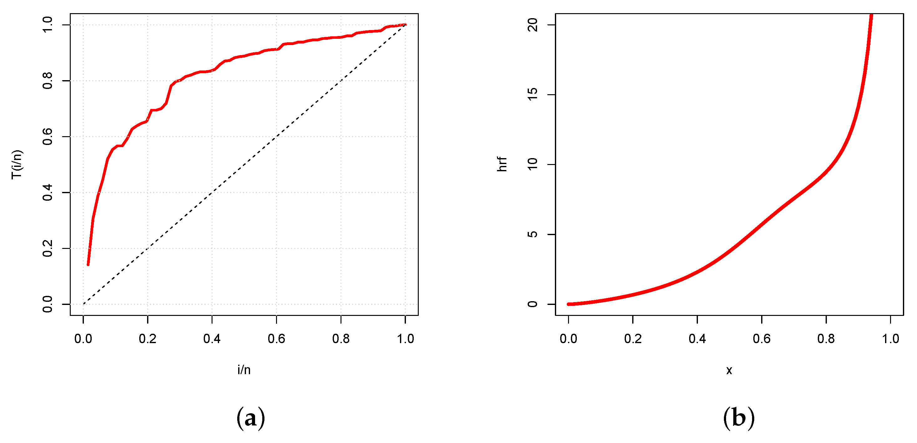
Now, we are conducting an hrf analysis. The total time test (TTT) plot is a useful graphical tool for determining whether or not data may be applied to a certain distribution through the underlying hrf. It has been elaborated by [23]. Figure 9 presents the TTT plot and the estimated hrf of the UG/G model.

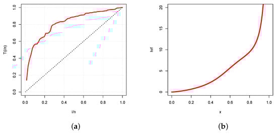
Figure 9. Plots of the (a) TTT plot and (b) estimated hrf of the UG/G model for the trade share data set.

In Figure 9a, the TTT plot indicates an increasing hrf, which is immediately confirmed in Figure 9b by the plot of the estimated hrf of the UG/G model.

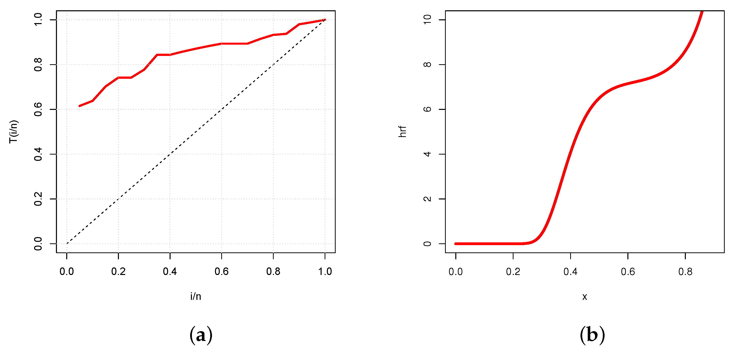
Again, the TTT plot in Figure 10a reveals an increasing hrf with diverse convex properties, which is immediately corroborated in Figure 10b by the plot of the estimated hrf of the UG/G model.

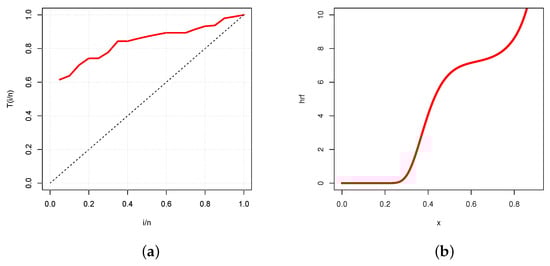
Figure 10. Plots of the (a) TTT plot and (b) estimated hrf of the UG/G model for the flood level data set.

This new study verifies the use of the UG/G model in the analysis of the data sets in question.

6. Conclusions

This work has provided a new option for unit distribution based on the inverse-exponential scheme and the gamma/Gompertz distribution. The basic aim was to translate the relevant flexibility of the gamma/Gompertz distribution to the unit interval. The unit gamma/Gompertz distribution is thus created. It can also be viewed as a natural extension of the power distribution, and the unit version of the Marshall–Olkin extended power distribution. As the main motivation, the proposed distribution has numerous advantages over referenced unit distributions in terms of flexibility and modeling capacities. Among them, its probability density function is shown to be increasing, decreasing, “increasing-decreasing”, and “decreasing-increasing” with a tuning asymmetry, and the hazard rate function has a monotonically increasing, decreasing, or constant form. Significant stochastic ordering, moments, and quantiles results have been demonstrated. In addition, a part has been devoted to the reliability coefficient with discussion on its inferential aspect. The new strategy is also applied practically with the development of the maximum likelihood method and two applications employing real data sets. The obtained results highlight the importance of the novel model. Future research in this direction will include, among other things, the development of quantile regression models and the construction of various dependence structures based on copulas.

References

- Aitchison, J. The statistical analysis of compositional data. J. R. Stat. Soc. Ser. B (Methodol.) 1982, 44, 139–177. [Google Scholar] [CrossRef]
- Consul, P.C.; Jain, G.C. On the log-gamma distribution and its properties. Stat. Pap. 1971, 12, 100–106. [Google Scholar] [CrossRef]
- Gómez-Déniz, E.; Sordo, M.A.; Calderín-Ojeda, E. The log-Lindley distribution as an alternative to the beta regression model with applications in insurance. Insur. Math. Econ. 2014, 54, 49–57. [Google Scholar] [CrossRef]
- Mazucheli, J.; Menezes, A.F.B.; Ghitany, M.E. The unit-Weibull distribution and associated inference. J. Appl. Probab. Stat. 2018, 13, 1–22. [Google Scholar]
- Mazucheli, J.; Menezes, A.F.B.; Fernandes, L.B.; De Oliveira, R.P.; Ghitany, M.E. The unit-Weibull distribution as an alternative to the Kumaraswamy distribution for the modeling of quantiles conditional on covariates. J. Appl. Stat. 2020, 47, 954–974. [Google Scholar] [CrossRef]
- Mazucheli, J.; Menezes, A.F.B.; Dey, S. Unit-Gompertz Distrib. Applications. Statistica 2019, 79, 25–43. [Google Scholar]
- Korkmaz, M.Ç.; Chesneau, C. On the unit Burr-XII distribution with the quantile regression modeling and applications. Comput. Appl. Math. 2021, 40, 29. [Google Scholar] [CrossRef]
- Altun, E. The log-weighted exponential regression model: Alternative to the beta regression model. Commun. Stat.-Theory Methods 2021, 50, 2306–2321. [Google Scholar] [CrossRef]
- Altun, E.; Hamedani, G.G. The log-xgamma distribution with inference and application. J. De La Société Française De Stat. 2018, 159, 40–55. [Google Scholar]
- Bantan, R.A.R.; Chesneau, C.; Jamal, F.; Elgarhy, M.; Tahir, M.H.; Aqib, A.; Zubair, M.; Anam, S. Some new facts about the unit-Rayleigh distribution with applications. Mathematics 2020, 8, 1954. [Google Scholar] [CrossRef]
- Bemmaor, A.C.; Glady, N. Modeling purchasing behavior with sudden “death”: A flexible customer lifetime model. Manag. Sci. 2012, 58, 1012–1021. [Google Scholar] [CrossRef]
- Afshar-Nadjafi, B. An iterated local search algorithm for estimating the parameters of the gamma/Gompertz distribution. Model. Simul. Eng. 2014, 2014, 629693. [Google Scholar] [CrossRef] [Green Version]
- Okagbue, H.I.; Adamu, M.O.; Owoloko, E.A.; Opanuga, A.A. Classes of ordinary differential equations obtained for the probability functions of Gompertz and gamma Gompertz distributions. In Proceedings of the World Congress on Engineering and Computer Science 2017, San Francisco, CA, USA, 25–27 October 2017; pp. 405–411. [Google Scholar]
- AzZwideen, R.; Al-Zou’bi, L.M. The transmuted gamma-Gompertz distribution. Int. J. Res.-Granthaalayah 2020, 8, 236–248. [Google Scholar] [CrossRef]
- Okorie, I.E.; AKpanta, A.C.; Ohakwe, J. Marshall-Olkin extended power function distribution. Eur. J. Stat. Probab. 2017, 5, 16–29. [Google Scholar]
- Shaked, M.; Shanthikumar, J.G. Stochastic Orders; Wiley: New York, NY, USA, 2007. [Google Scholar]
- Gilchrist, W. Statistical Modelling with Quantile Functions; CRC Press: Abingdon, UK, 2000. [Google Scholar]
- Kotz, S.; Lumelskii, Y.; Pensky, M. The Stress-Strength Model and Its Generalizations: Theory and Applications; World Scientific: Singapore, 2003. [Google Scholar]
- Casella, G.; Berger, R.L. Statistical Inference; Brooks/Cole Publishing Company: Bel Air, CA, USA, 1990. [Google Scholar]
- R Core Team. R: A Language and Environment for Statistical Computing; R Foundation for Statistical Computing: Vienna, Austria, 2013; Available online: http://www.R-project.org/ (accessed on 20 February 2021).
- Stock, J.H.; Watson, M.W. Introduction to Econometrics, 2nd ed.; Addison Wesley: Boston, MA, USA, 2007; Available online: https://rdrr.io/cran/AER/man/GrowthSW.html (accessed on 20 June 2020).
- Dumonceaux, R.; Antle, C.E. Discrimination between the Log-Normal and the Weibull distributions. Technometrics 1973, 15, 923–926. [Google Scholar] [CrossRef]
- Aarset, M.V. How to identify bathtub hazard rate. IEEE Trans. Reliab. 1987, 36, 106–108. [Google Scholar] [CrossRef]
Publisher’s Note: MDPI stays neutral with regard to jurisdictional claims in published maps and institutional affiliations. |
© 2021 by the authors. Licensee MDPI, Basel, Switzerland. This article is an open access article distributed under the terms and conditions of the Creative Commons Attribution (CC BY) license (https://creativecommons.org/licenses/by/4.0/).