A Dynamic Multi-Objective Duopoly Game with Capital Accumulation and Pollution

Abstract

This paper studies a discrete-time dynamic duopoly game with homogenous goods. Both firms have to decide on investment where investment increases production capacity so that they are able to put a larger quantity on the market. The downside, however, is that a larger quantity raises pollution. The firms have multiple objectives in the sense that each one maximizes the discounted profit stream and appreciates a clean environment as well. We obtain some surprising results. First, where it is known from the continuous-time differential game literature that firms invest more under a feedback information structure compared to an open-loop one, we detect scenarios where the opposite holds. Second, in a feedback Nash equilibrium, capital stock is more sensitive to environmental appreciation than in the open-loop case.

1. Introduction

Corporate social responsibility (CSR) emphasizes that a firm does not just care about profit maximization, but has at the same time other objectives in mind that benefit society. According to Wirl et al. [1], examples of CSR projects are environmental reports, philanthropic support and sponsoring, energy and environmental management, mentoring and educational programs for workers, family-friendly workplaces and more. Wirl et al. [1] studied a dynamic model where a firm optimizes over CSR activities. Lambertini et al. [2] consider CSR activities in a strategic setting. In particular, a Cournot game is designed where one firm, as usual, maximizes profits, but where the other firm is a CSR firm in the sense that consumer surplus and pollution are also taken into account. Lambertini et al. [2] reach the surprising result that, provided the market is sufficiently large, the CSR firm earns higher profits. Yanase [3] also considers CSR activities but in that sense solely concentrates on the environment. The study investigates how an increase in the firms’ environmental consciousness affects the environment and economic welfare. Feichtinger et al. [4] take a similar approach by analyzing a dynamic oligopoly in which environmental externalities are taken into account in the firms’ objectives.

Our paper studies a dynamic duopoly in which the firms accumulate capital. The positive side is that with the capital stock firms can produce goods which can be sold on the market, resulting in firm profits. The negative side is that the production process of both firms causes pollution. As in the literature just mentioned, the firm takes both these elements explicitly into account. The new element of our research, however, is that we take a multi-objective approach, in that at the same time firms strive to maximize profits and minimize pollution (the different weights between the two objectives are not a priori fixed). In so doing, we obtain the new result that, compared to an open-loop information structure, in a feedback Nash equilibrium the firms are less sensitive to changes in environmental appreciation.

Our approach is close to albeit different from that of Rettieva [5]. She considers a dynamic, discrete time, two-player game model where the players use a common resource. Both players have two goals to optimize over an infinite horizon, namely maximizing profit from selling fish and minimizing catching costs (the value of those costs depends on both players’ catches). (She also studies the case where the players have different random horizons.) She introduces an original version of the Nash bargaining scheme (one for each goal), where status quo points are computed in different cases. (Those cases refer to different instances of zero-sum games.) Multi-criteria cooperative equilibria are considered by Rettieva [6].

Our contribution differs in several ways from that of Rettieva. First, we are interested in a pollution-control problem, and not in a resource-management problem. Second, we do not rely on the Nash bargaining approach; we follow an approach that can be loosely called Nash equilibrium with Pareto equilibrium. More precisely, in equilibrium each firm chooses a Pareto-optimal solution to its multi-objective problem. Third, among the objectives pursued by the players, one is especially environmental (whereas we may think that in Rettieva’s setting players actually have two economic objectives). (This paper is related to, but also differs from, the papers by Kuzyutin, Gromova and Pankratova [7,8] who develop a cooperative game theory approach of dynamic multi-criteria decision analysis and who pay special attention to the time-consistency issue).

Our paper is also connected to the work of Crettez and Hayek (2021) [9] who study a dynamic Cournot duopoly where production causes pollution, albeit without capital accumulation. They notably show that contrary to the case where the firms’ objective just concerns profit maximization, there exist Nash equilibria where production is lower than in the cooperative equilibrium. (In our setting, when firms have a unique objective, cooperating means behaving like a monopolist. A monopolist usually reduces production in order to raise the price of its product.) This stems from the fact that in a Nash equilibrium firms do not coordinate on the choice of the relative weight given to the environmental objective. This result highlights the fact that when firms pursue multiple and separate objectives, equilibrium behavior can display an over-reaction. In this paper, we also obtain this form of over-compliance. Here, however, open-loop equilibria differ from feedback equilibria, whereas in the work of Crettez and Hayek [9], open-loop equilibria are all feedback.

In addition to the literature that studies corporate social responsibility within a dynamic framework, our paper is also connected to straightforward capital accumulation models where firms maximize profits. A seminal paper in that area is that of Reynolds (1987) [10] who finds, as a major result, that firms invest more under a feedback information structure than under an open-loop one. If firms put the environmental weights to zero, we in fact have the same problem as in the work of Reynolds [10]. However, there is a difference, because where Reynolds [10] studies a continuous time framework, our model is in discrete time. Very surprisingly, it turns out that we find scenarios where in the long run the open-loop equilibrium admits steady state capital stocks that are bigger than in the feedback case.

Other approaches of multiple objective games and Stackelberg games can be found in recent publications such as [11,12,13,14,15].

The paper is organized as follows. Section 2 presents the model. Section 3 and Section 4 develop the open loop and the feedback Nash equilibria, respectively. The cooperative equilibrium is analyzed in Section 5. Section 6 compares the different equilibrium outcomes and Section 7 concludes the paper.

2. Model

Consider a dynamic duopoly where firms produce the same type of goods and where the inverse demand function at date t is given by

$$\begin{array}{c}\hfill p(q_{1t},q_{2t})=max\left\{0,a-b(q_{1t}+q_{2t})\right\},a>0,b>0.\end{array}$$

In the expression above, $q_{it}$ denotes the quantity supplied by firm i at date t, a is the maximum willingness to pay for the product and b represents the sensibility of the market price to the volume of production brought to the market. (We shall always assume that $p(q_{1t},q_{2t})$ is strictly positive. We can also interpret a as being the maximum willingness to pay minus the average production cost (in that case, we assume that this average cost is constant)).

For simplicity, production is proportional to the stock of capital $K_{it}$ held by each firm i at date t, and we set the proportionality coefficients equal to one: $q_{it}=K_{it}$. The law of motion of the capital stock is as follows

$$\begin{array}{c}\hfill K_{it+1}=I_{it}+(1-\delta )K_{it},\end{array}$$

(1)

where $I_{it}$ is the investment rate of firm i at date t, and $\delta$ is a depreciation rate ($0<\delta <1$). (This is a discrete-time variant of the model proposed by Reynolds [10] (see also Lambertini (2018) [16] p. 73).) We assume that it costs $\frac{I_{it}^2}{2}$ for firm i to decrease/increase its capital stock by an amount $I_{it}$ (in the event that $I_{it}<0$, we have $I_{it}\ge -(1-\delta )K_{it}$).

Production is a polluting activity. To simplify the analysis, we suppose that emissions are equal to total production, i.e., $q_{1t}+q_{2t}$, and that the dynamics of the pollution stock $x_t$ is written as follows

$$\begin{array}{c}\hfill x_{t+1}=\eta x_t+q_{1t}+q_{2t},\end{array}$$

(2)

where $0<1-\eta <1$ is the natural decay rate of pollution, and $x_0$, the initial value of pollution, is given.

Firm i’s objective is given by the following multi-objective program.

$$\underset{{(I_{it})}_t}{max}\left\{\sum _{t=0}^{\infty }{\beta }^t\left(a-b\left(K_{it}+K_{3-it}\right)K_{it}-\frac{I_{it}^2}{2}\right),-\sum _0^{\infty }{\beta }^t{x}_t\right\}$$

(3)

subject to

$$\begin{array}{cc}\hfill K_{it+1}& =I_{it}+(1-\delta )K_{it},\hfill \end{array}$$

(4)

$$\begin{array}{cc}\hfill x_{t+1}& =\eta x_t+K_{it}+K_{3-it},\hfill \end{array}$$

(5)

$$\begin{array}{cc}\hfill I_{it}& \ge -(1-\delta )K_{it},\hfill \end{array}$$

(6)

$$\begin{array}{cc}\hfill x_0& ,K_{i0},\mathrm{and}{(K_{3-it})}_t\mathrm{being}\mathrm{given},\hfill \end{array}$$

(7)

In the program above, ${(K_{3-it})}_t$ is a bounded sequence such that $0\le K_{3-it}\le a$ for all t. The meaning of the program above is that firm i tries to maximize the value of its profit ${\sum }_0^{\infty }{\beta }^t(a-b(K_{it}+K_{3-it})K_{it}-\frac{I_{it}^2}{2})$ where $\beta$ is a discount factor such that $0<\beta <1$, and to minimize ${\sum }_0^{\infty }{\beta }^t{x}_t$, a measure of intertemporal pollution. For simplicity again, in this measure future values of pollution are discounted at the same rate as future receipts.

3. Open-Loop Nash Equilibria

We next state the definition of an open-loop equilibrium for our dynamic game.

Definition 1.

A Nash equilibrium is a sequence of decisions ${({\widehat{I}}_{1t},{\widehat{I}}_{2t})}_t$ such that ${({\widehat{I}}_{it})}_t$ is a solution to problems (3)–(7) when ${({\widehat{I}}_{3-it})}_t$ is given, $i=1,2$.

Notice that the sequence ${({\widehat{I}}_{3-it})}_t$ determines the sequence of ${({\widehat{K}}_{3-it})}_t$ that is supposed to be given in problem (3)–(7).

Before presenting optimality conditions for an open-loop Nash equilibrium, notice that in any equilibrium each firm chooses a Pareto-optimal solution to its multi-objective problem. (This is why some authors call Nash equilibria for multi-objective games Pareto-Nash equilibria. See, e.g., Qu and Ji (2016) [17] Section 1.2 for a quick literature review.) As a consequence, in any equilibrium each firm gives a relative weight to its environmental objective. In the sequel, we will denote by ${\lambda }_2$ the relative weight of the environmental objective of firm 1 and by ${\gamma }_2$ the corresponding relative weight of firm 2. Of course, not all pairs of weights $({\lambda }_2,{\gamma }_2)$ will be admissible in equilibrium.

3.1. Optimality Conditions

The next result determines the set of equilibrium weights given by the two firms to their environmental objectives as well as the equilibrium investment rates.

Proposition 1.

For each pair $({\lambda }_2,{\gamma }_2)$ of relative weights given to the environmental objectives of firms 1 and 2, respectively, satisfying the following conditions

$$\frac{\beta {\lambda }_2}{1-\beta \eta }\left(2b+\delta (\frac{1}{\beta }-1+\delta )\right)-\frac{b\beta {\gamma }_2}{1-\beta \eta }<a\left(b+\delta (\frac{1}{\beta }-1+\delta )\right),$$

(8)

$$\frac{\beta {\gamma }_2}{(1-\beta \eta )}\left(2b+\delta (\frac{1}{\beta }-1+\delta )\right)-\frac{b\beta {\lambda }_2}{(1-\beta \eta )}<a\left(b+\delta (\frac{1}{\beta }-1+\delta )\right),$$

(9)

there is an open-loop Nash equilibrium ${(I_{1t},I_{2t})}_t$ such that $I_{it}>-(1-\delta )K_{it}$, $i=1,2$, with

$$\begin{array}{c}{I}_{1t}=\frac{K_{10}}{2}\left(r_1^t\left(r_1-(1-\delta )\right)+s_1^t\left(s_1-(1-\delta )\right)\right)+D^1\left(1-s_1^{t+1}-(1-\delta )(1-s_1^t)\right)\hfill \\ \hfill +\frac{K_{20}-C}{2}\left(r_1^t\left(r_1-(1-\delta )\right)-s_1^t\left(s_1-(1-\delta )\right)\right).\end{array}$$

(10)

$$\begin{array}{c}{I}_{2t}=\frac{K_{20}}{2}\left(r_1^t\left(r_1-(1-\delta )\right)+s_1^t\left(s_1-(1-\delta )\right)\right)+D^2\left(1-s_1^{t+1}-(1-\delta )(1-s_1^t)\right)\hfill \\ \hfill +\frac{K_{10}-C}{2}\left(r_1^t\left(r_1-(1-\delta )\right)-s_1^t\left(s_1-(1-\delta )\right)\right),\end{array}$$

(11)

where

$$C=\frac{2a-\frac{({\lambda }_2+{\gamma }_2)\beta }{1-\beta \eta }}{\delta (-1+\delta +1/\beta )+3b},$$

$$D^1=\frac{a-bC-\frac{{\lambda }_2\beta }{1-\beta \eta }}{\delta (-1+\delta +1/\beta )+b},D^2=\frac{a-bC-\frac{{\gamma }_2\beta }{1-\beta \eta }}{\delta (-1+\delta +1/\beta )+b},$$

$$r_1=\frac{{(1-\delta )}^2+3b+1/\beta -\sqrt{\Delta }}{2(1-\delta )},$$

$$s_1=\frac{{(1-\delta )}^2+b+1/\beta -\sqrt{{\Delta }^{\prime }}}{2(1-\delta )},$$

$$\Delta ={({(1-\delta )}^2+3b+1/\beta )}^2-4{(1-\delta )}^2/\beta$$

$${\Delta }^{\prime }={({(1-\delta )}^2+b+1/\beta )}^2-4{(1-\delta )}^2/\beta .$$

The equilibrium values of and $K_{1t},K_{2t},x_t$ are given by

$$\begin{array}{cc}\hfill K_{1t}& =K_{10}\frac{(r_1^t+s_1^t)}{2}+D^1(1-s_1^t)+\frac{(K_{20}-C)}{2}(r_1^t-s_1^t),\hfill \end{array}$$

(12)

$$\begin{array}{cc}\hfill K_{2t}& =K_{20}\frac{(r_1^t+s_1^t)}{2}+D^2(1-s_1^t)+\frac{(K_{10}-C)}{2}(r_1^t-s_1^t),\hfill \end{array}$$

(13)

$$\begin{array}{cc}\hfill x_t& ={\eta }^t(x_0-\frac{K_{10}+K_{20}-C}{r_1-\eta }-\frac{C}{1-\eta })+r_1^t\frac{K_{10}+K_{20}-C}{r_1-\eta }+\frac{C}{1-\eta }.\hfill \end{array}$$

(14)

Proof. 

From Theorem 4.2 in the work of Hayek [18], we know that if a bounded sequence ${(I_{1t})}_t$ is a solution to problem (3)–(7) such that $I_{1t}>-(1-\delta )K_{1t}$, then there exist ${\lambda }_1\ge 0,{\lambda }_2\ge 0$, ${({\mu }_t)}_t$ in ${\ell }^1$ (the set of sequence ${(x_t)}_t$ such that ${\sum }_{t=0}^{\infty }\left|x_t\right|$ is a real number), ${({\psi }_t)}_t$ in ${\ell }^1$, not all nil, such that any each date, ${(I_{1t})}_t$ maximizes the following Hamiltonian, given ${(I_{2t},K_{2t})}_t$:

$$\begin{array}{cc}\hfill H(I_{1t},K_{1t},x_t,{\lambda }_1,{\lambda }_2,{\mu }_t,{\psi }_t)& ={\lambda }_1({\beta }^t(a-b(K_{1t}+K_{2t})K_{1t}-\frac{I_{1t}^2}{2})+{\lambda }_2(-{\beta }^t{x}_t)\hfill \\ \hfill & +{\mu }_{t+1}(\eta x_t+K_{1t}+K_{2t})+{\psi }_{t+1}\left(I_{1t}+(1-\delta )K_{1t}\right)\hfill \end{array}$$

The first-order conditions are given by

$$\begin{array}{cc}\hfill 0& =-{\lambda }_1{\beta }^t{I}_{1t}+{\psi }_{t+1},\hfill \end{array}$$

(15)

$$\begin{array}{cc}\hfill {\psi }_t& ={\lambda }_1{\beta }^t\left(a-2b{K}_{1t}-b{K}_{2t}\right)+{\mu }_{t+1}+(1-\delta ){\psi }_{t+1},\hfill \end{array}$$

(16)

$$\begin{array}{cc}\hfill {\mu }_t& =-{\lambda }_2{\beta }^t+\eta {\mu }_{t+1}.\hfill \end{array}$$

(17)

The last two equations refer to the dynamics of the shadow values ${\psi }_t$ and ${\mu }_t$ of the capital stock and pollution, respectively.

Note that since ${({\mu }_t)}_t$ in ${\ell }^1$, ${({\psi }_t)}_t$ in ${\ell }^1$, the familiar transversality condition is necessarily satisfied.

Since H is concave in $(I_t,K_t)$ and since the familiar transversality condition is satisfied, the first-order conditions above are sufficient. We now study these conditions in detail.

Observe that ${\lambda }_1\ne 0$. Otherwise, we would have ${\psi }_{t+1}=0$ for all t, which in turn would yield ${\mu }_{t+1}=0$ for all t, so that ${\lambda }_2=0$. All those variables would be nil, which is impossible.

By a standard argument, we obtain

$$\begin{array}{cc}\hfill {\mu }_t& =-\frac{{\lambda }_2{\beta }^t}{1-\beta \eta }.\hfill \end{array}$$

(18)

The following dynamic system obtained from Equations (1), (2) and (15)–(17) remains to be solved. (Its solution will be an open-loop Nash equilibrium since the Hamiltonians are concave and the transversality condition is satisfied).

$$\begin{array}{cc}\hfill {\psi }_t& ={\lambda }_1{\beta }^t\left(a-2b{K}_{1t}-b{K}_{2t}\right)-\frac{{\lambda }_2{\beta }^{t+1}}{1-\beta \eta }+(1-\delta ){\psi }_{t+1}\hfill \end{array}$$

(19)

$$\begin{array}{cc}\hfill K_{1t+1}& =\frac{{\psi }_{t+1}}{{\lambda }_1{\beta }^t}+(1-\delta )K_{1t},\hfill \end{array}$$

(20)

$$\begin{array}{cc}\hfill x_{t+1}& =\eta x_t+K_{1t}+K_{2t}.\hfill \end{array}$$

(21)

Since ${\lambda }_1>0$, we can set ${\lambda }_1=1$. Defining $\frac{{\psi }_t}{{\beta }^t}={\Psi }_t$, Equations (19) and (20) can be written as

$$\begin{array}{cc}\hfill {\Psi }_t& =a-2b{K}_{1t}-b{K}_{2t}-\frac{\beta {\lambda }_2}{1-\beta \eta }+\beta (1-\delta ){\Psi }_{t+1},\hfill \end{array}$$

(22)

$$\begin{array}{cc}\hfill K_{1t+1}& =\beta {\Psi }_{t+1}+(1-\delta )K_{1t},\hfill \end{array}$$

(23)

Combining the two equations above, we obtain

$$\begin{array}{cc}\hfill \frac{K_{1t}-(1-\delta )K_{1t-1}}{\beta }& =\left(a-2b{K}_{1t}-b{K}_{2t}\right)-\frac{\beta {\lambda }_2}{1-\beta \eta }+\beta (1-\delta )\frac{K_{1t+1}-(1-\delta )K_{1t}}{\beta }.\hfill \end{array}$$

(24)

Rearranging, we obtain

$$(1-\delta )K_{1t+1}-K_{1t}\left({(1-\delta )}^2+2b+1/\beta \right)+(1-\delta )K_{1t-1}/\beta =-a+b{K}_{2t}+\frac{\beta {\lambda }_2}{1-\beta \eta }$$

or

$$\begin{array}{c}\hfill (1-\delta )K_{1t+2}-K_{1t+1}\left({(1-\delta )}^2+2b+1/\beta \right)+(1-\delta )K_{1t}/\beta =-a+b{K}_{2t+1}+\frac{\beta {\lambda }_2}{1-\beta \eta }\end{array}$$

(25)

This equation also holds for firm $3-i$. By considering symmetry and taking the optimality conditions for both firms into account, we obtain

$$(1-\delta )(K_{1t+2}+K_{2t+2})-(K_{1t+1}+K_{2t+1})\left({(1-\delta )}^2+3b+1/\beta \right)+(1-\delta )(K_{1t}+K_{2t})/\beta$$

$$=-2a+\frac{\beta ({\lambda }_2+{\gamma }_2)}{1-\beta \eta }.$$

Set $Z_t=K_{1t}+K_{2t}$. We obtain:

$$(1-\delta )Z_{t+2}-Z_{t+1}\left({(1-\delta )}^2+3b+1/\beta \right)+(1-\delta )Z_t/\beta$$

$$=-2a+\frac{\beta ({\lambda }_2+{\gamma }_2)}{1-\beta \eta }$$

Define:

$$\begin{array}{cc}\hfill \Delta & ={\left({(1-\delta )}^2+3b+1/\beta \right)}^2-4{(1-\delta )}^2/\beta \hfill \\ \hfill & =\left({(1-\delta )}^2+3b+1/\beta -2(1-\delta )/\sqrt{\beta }\right)\left({(1-\delta )}^2+3b+1/\beta +2(1-\delta )/\sqrt{\beta }\right)>0\hfill \end{array}$$

since the expression ${(1-\delta )}^2+3b+1/\beta -2(1-\delta )/\sqrt{\beta }>0$, being a decreasing function of $\beta$ which is positive for $\beta =1$.

Solving the above difference equation, we obtain $Z_t=c_1{r}_1^t+c_2{r}_2^t+C$, where

$$\begin{array}{cc}\hfill C& :=\frac{-2a+\frac{({\lambda }_2+{\gamma }_2)\beta }{1-\beta \eta }}{(1-\delta )-({(1-\delta )}^2+3b+1/\beta )+(1-\delta )/\beta }\hfill \\ \hfill & =\frac{-2a+\frac{({\lambda }_2+{\gamma }_2)\beta }{1-\beta \eta }}{(1-\delta )-({(1-\delta )}^2+3b)-\delta /\beta }=\frac{-2a+\frac{({\lambda }_2+{\gamma }_2)\beta }{1-\beta \eta }}{\delta (1-\delta -1/\beta )-3b}\hfill \\ \hfill & =\frac{2a-\frac{({\lambda }_2+{\gamma }_2)\beta }{1-\beta \eta }}{\delta (-1+\delta +1/\beta )+3b}.\hfill \end{array}$$

(26)

Moreover,

$$\begin{array}{cc}\hfill r_1& =\frac{{(1-\delta )}^2+3b+1/\beta -\sqrt{\Delta }}{2(1-\delta )}\hfill \end{array}$$

(27)

$$\begin{array}{cc}\hfill & =\frac{2(1-\delta )}{\beta [{(1-\delta )}^2+3b+1/\beta +\sqrt{\Delta }]}\hfill \end{array}$$

(28)

$$\begin{array}{cc}\hfill r_2& =\frac{{(1-\delta )}^2+3b+1/\beta +\sqrt{\Delta }}{2(1-\delta )}\hfill \end{array}$$

(29)

$$\begin{array}{cc}\hfill Z_t& =c_1{r}_1^t+c_2{r}_2^t+C.\hfill \end{array}$$

(30)

Observe that $r_1{r}_2=1/\beta >1$ and $r_2>1$. We also have $r_1<1$.

To show that $r_1<1$, we shall prove that ${(1-\delta )}^2+3b+1/\beta -\sqrt{\Delta }<2(1-\delta )$. We have

$${(1-\delta )}^2+3b+1/\beta -2(1-\delta )<\sqrt{\Delta }$$

$$⟺{({(1-\delta )}^2+3b+1/\beta -2(1-\delta ))}^2{<\Delta (\mathrm{since}(1-\delta )}^2+3b+1/\beta -2(1-\delta )>0$$

$$⟺{({(1-\delta )}^2+3b+1/\beta )}^2-4(1-\delta )({(1-\delta )}^2+3b+1/\beta )+4{(1-\delta )}^2<{({(1-\delta )}^2+3b+1/\beta )}^2-4{(1-\delta )}^2/\beta$$

$$⟺\delta (1-\delta )-(3b+1/\beta )<-(1-\delta )/\beta$$

$$⟺\delta (1-\delta -1/\beta )-3b<0$$

In this case, since $Z_t$ is bounded, we have $c_2=0$ and $Z_t=c_1{r}_1^t+C$.

Notice that $Z_t>0$ if

$$C>0\iff {\lambda }_2+{\gamma }_2<\frac{2a(1-\beta \eta )}{\beta }.$$

The right condition holds since it is implied by conditions (8) and (9).

Then, $Z_t=c_1{r}_1^t+C=(Z_0-C)r_1^t+C=(K_{10}+K_{20}-C)r_1^t+C=(K_{10}+K_{20})r_1^t+C(1-r_1^t)>0$.

Now, setting $K_{2t+1}=Z_{t+1}-K_{1t+1}$ in Equation (25), we obtain

$$(1-\delta )K_{1t+2}-K_{1t+1}\left({(1-\delta )}^2+b+1/\beta \right)+(1-\delta )K_{1t}/\beta =-a+b{Z}_{t+1}+\frac{\beta {\lambda }_2}{1-\beta \eta }$$

or

$$(1-\delta )K_{1t+2}-K_{1t+1}\left({(1-\delta )}^2+b+1/\beta \right)+(1-\delta )K_{1t}/\beta =-a+b{c}_1{r}_1^{t+1}+bC+\frac{\beta {\lambda }_2}{1-\beta \eta }.$$

Solving the above difference equation we obtain $K_{1t}=d_1{s}_1^t+d_2{s}_2^t+D_t$ where

$$D_t=\frac{-a+bC+\frac{{\lambda }_2\beta }{1-\beta \eta }}{(1-\delta )-({(1-\delta )}^2+b+1/\beta )+(1-\delta )/\beta }$$

$$+\frac{b{c}_1}{((1-\delta )r_1^2-({(1-\delta )}^2+b+1/\beta )r_1+(1-\delta )/\beta )}{r}_1^{t+1}.$$

By definition of $r_1$, we have

$$\begin{array}{c}\hfill (1-\delta )r_1^2-\left({(1-\delta )}^2+3b+\frac{1}{\beta }\right)r_1+\frac{(1-\delta )}{\beta }=0.\end{array}$$

(31)

Therefore, the denominator in the fraction above reduces to $2b{r}_1$ and thus

$$D_t=\frac{a-bC-\frac{{\lambda }_2\beta }{1-\beta \eta }}{\delta (-1+\delta +1/\beta )+b}+\frac{c_1}{2}{r}_1^t=D^1+\frac{c_1}{2}{r}_1^t$$

where

$$\begin{array}{cc}\hfill D^1& =\frac{a-bC-\frac{{\lambda }_2\beta }{1-\beta \eta }}{\delta (-1+\delta +1/\beta )+b}.\hfill \end{array}$$

(32)

Notice that

$$\begin{array}{cc}\hfill {\Delta }^{\prime }& ={\left({(1-\delta )}^2+b+1/\beta \right)}^2-4{(1-\delta )}^2/\beta >0\hfill \\ \hfill s_1& =\frac{{(1-\delta )}^2+b+1/\beta -\sqrt{{\Delta }^{\prime }}}{2(1-\delta )}=\frac{2(1-\delta )}{\beta [{(1-\delta )}^2+b+1/\beta +\sqrt{{\Delta }^{\prime }}]}\hfill \\ \hfill s_2& =\frac{{(1-\delta )}^2+b+1/\beta +\sqrt{{\Delta }^{\prime }}}{2(1-\delta )}.\hfill \end{array}$$

We observe again that $s_1{s}_2=1/\beta >1$, $s_2>1$ and $s_1<1$.

In this case, since $K_{1t}$ is bounded we have $d_2=0$ and $K_{1t}=d_1{s}_1^t+D_t$ and we have $K_{2t}=Z_t-K_{1t}$. More precisely, $d_1=K_{10}-D_0$ and

$$\begin{array}{cc}\hfill D_0& =D^1+\frac{c_1}{2},\hfill \end{array}$$

(33)

where $c_1=(K_{10}+K_{20}-C)$.

We therefore obtain:

$$\begin{array}{cc}\hfill K_{1t}& =d_1{s}_1^t+D_t\hfill \\ \hfill & =(K_{10}-D_0)s_1^t+D^1+\frac{c_1}{2}{r}_1^t\hfill \\ \hfill & =(K_{10}-(D^1+\frac{c_1}{2}))s_1^t+D^1+\frac{c_1}{2}{r}_1^t\hfill \\ \hfill & =(K_{10}-D^1)s_1^t+D^1+\frac{c_1}{2}{r}_1^t-\frac{c_1}{2}{s}_1^t\hfill \\ \hfill & =K_{10}{s}_1^t+D^1(1-s_1^t)+\frac{(K_{10}+K_{20}-C)}{2}(r_1^t-s_1^t)\hfill \\ \hfill & =K_{10}\frac{(r_1^t+s_1^t)}{2}+D^1(1-s_1^t)+\frac{(K_{20}-C)}{2}(r_1^t-s_1^t).\hfill \end{array}$$

(34)

We now must make sure that $K_{1\infty }>0$. This implies that $D^1>0$. Using the expressions of $D^1$ and C, we obtain that $D^1>0$ if and only if:

$$\frac{\beta {\lambda }_2}{1-\beta \eta }\left(2b+\delta (-1+\delta +\frac{1}{\beta })\right)-\frac{b\beta {\gamma }_2}{1-\beta \eta }<a\left(b+\delta (-1+\delta +\frac{1}{\beta })\right).$$

(35)

which is condition (8). We obtain $K_{2t}$ by subtracting $K_{1t}$ from $Z_t$.

$$\begin{array}{cc}\hfill K_{2t}& =(K_{10}+K_{20})r_1^t+C(1-r_1^t)-\left(K_{10}\frac{(r_1^t+s_1^t)}{2}+D^1(1-s_1^t)+\frac{(K_{20}-C)}{2}(r_1^t-s_1^t)\right)\hfill \\ \hfill & =K_{20}\frac{(r_1^t+s_1^t)}{2}+C-D^1(1-s_1^t)+\frac{(-C)}{2}(r_1^t+s_1^t)+\frac{(K_{10})}{2}(r_1^t-s_1^t)\hfill \\ \hfill & =K_{20}\frac{(r_1^t+s_1^t)}{2}+(C-D^1)(1-s_1^t)+\frac{(K_{10}-C)}{2}(r_1^t-s_1^t)\hfill \\ \hfill & =K_{20}\frac{(r_1^t+s_1^t)}{2}+D^2(1-s_1^t)+\frac{(K_{10}-C)}{2}(r_1^t-s_1^t).\hfill \end{array}$$

(36)

where $D^2=C-D^1=\frac{a-bC-\frac{{\gamma }_2\beta }{1-\beta \eta }}{\delta (-1+\delta +1/\beta )+b}$ (where we have used Equations (26) and (32)).

We also have to make sure that $K_{2\infty }>0$. This implies that $C>D^1$. Using the expressions of C and $D^1$, this condition can be written as

$$\frac{\beta {\gamma }_2}{(1-\beta \eta )}\left(2b+\delta (\frac{1}{\beta }-1+\delta )\right)-\frac{b\beta {\lambda }_2}{(1-\beta \eta )}<a\left(b+\delta (\frac{1}{\beta }-1+\delta )\right).$$

(37)

which is condition (9).

Finally, we obtain $x_{t+1}=\eta x_t+K_{1t}+K_{2t}=\eta x_t+Z_t=\eta x_t+(K_{10}+K_{20}-C)r_1^t+C$ so

$$x_t={\eta }^t\left(x_0-\frac{K_{10}+K_{20}-C}{r_1-\eta }-\frac{C}{1-\eta }\right)+r_1^t\frac{K_{10}+K_{20}-C}{r_1-\eta }+\frac{C}{1-\eta }.$$

□

The proposition above shows that there are multiple interior Nash equilibria, each characterized by a pair of relative weights $({\lambda }_2,{\gamma }_2)$ given their environmental objectives.

Condition (8) defines an upper bound for the environmental appreciation parameter ${\lambda }_2$ such that the firm wants to be an active producer in the long run, translating into $K_{1t}>0$. Analogously, condition (9) is a similar condition for ${\gamma }_2$ with respect to the long run level of $K_2$. Furthermore, conditions (8) and (9) imply

$$\begin{array}{c}\hfill {\lambda }_2+{\gamma }_2<\frac{2a(1-\beta \eta )}{\beta },\end{array}$$

(38)

This condition ensures that $C>0$, so that in the long run $K_{1t}+K_{2t}$ is positive.

The above condition is clear: if both firms give too much weight to their environmental objective, then they do not need to accumulate capital, because doing so will lead to an increase in pollution. Condition (8) will hold for large a, because then the market is profitable. It will not hold for large ${\lambda }_2$, because firm 1 does not like to pollute and therefore reduces investments. It will hold for large ${\gamma }_2$. Then, firm 2 has less incentive to invest, which increases the output price for firm 1, making investment for firm 1 more profitable.

3.2. Sensitivity Analysis

Lemma 1.

Consider two open-loop Nash equilibria with different relative weights ${\lambda }_2$ given to the environmental objective of firm 1 and the same relative weight ${\gamma }_2$ given to the environmental objective of firm 2. Then, for every time instant, the capital stock of the first firm $K_{1t}$ is always lower in the equilibrium associated with the higher value of ${\lambda }_2$.

Proof. 

We show below that $\frac{\partial K_{1t}}{\partial {\lambda }_2}<0$.

Using Equation (34), we have

$$\frac{\partial K_{1t}}{\partial {\lambda }_2}=\frac{\partial D^1}{\partial {\lambda }_2}(1-s_1^t)-\frac{\partial C}{\partial {\lambda }_2}\frac{(r_1^t-s_1^t)}{2}$$

where

$$C=\frac{2a-(\frac{({\lambda }_2+{\gamma }_2)\beta }{1-\beta \eta })}{\delta (-1+\delta +1/\beta )+3b},D_1=\frac{a-bC-(\frac{{\lambda }_2\beta }{1-\beta \eta })}{\delta (-1+\delta +1/\beta )+b}.$$

Set $G=\delta (1-\delta -1/\beta )-b<0$.

$$\begin{array}{cc}\hfill \frac{\partial C}{\partial {\lambda }_2}& =\frac{-\beta }{(1-\beta \eta )[\delta (-1+\delta +1/\beta )+3b]}<0,\hfill \end{array}$$

(39)

$$\begin{array}{cc}\hfill \frac{\partial D^1}{\partial {\lambda }_2}& =[\frac{b\partial C}{\partial {\lambda }_2}+\frac{\beta }{1-\beta \eta }]/G.\hfill \end{array}$$

(40)

When t is large, the sign of $\frac{\partial K_{1t}}{\partial {\lambda }_2}$ is the same as that of $\frac{\partial D^1}{\partial {\lambda }_2}$. We obtain:

$$\begin{array}{cc}\hfill \frac{\partial D^1}{\partial {\lambda }_2}& =\frac{\beta }{(1-\beta \eta )G}\left[1-\frac{b}{\delta (-1+\delta +\frac{1}{\beta })+3b}\right]<0\hfill \end{array}$$

(41)

since

$$\begin{array}{cc}\hfill 1& >\frac{b}{\delta (-1+\delta +\frac{1}{\beta })+3b}.\hfill \end{array}$$

(42)

Moreover, this negative effect exists both in the short and the long run (because $-\frac{\partial C}{\partial {\lambda }_2}\frac{(r_1^t-s_1^t)}{2}<0$, since one can check that $r_1<s_1$). Therefore, we always have $\frac{\partial K_{1t}}{\partial {\lambda }_2}<0$. □

Notice that this is in contrast with the model without capital accumulation of Crettez and Hayek [9] where a change in ${\lambda }_2$ has an indeterminate effect on the production level.

Lemma 2.

Consider two open-loop Nash equilibria with different relative weights ${\gamma }_2$ given to the environmental objective of firm 2 and the same relative weight ${\lambda }_2$ given to the environmental objective of firm 1. Then, for every time instant, the capital stock of the first firm $K_{1t}$ is always higher in the equilibrium associated with the higher value of ${\gamma }_2$.

Proof. 

Using Equation (34), we have

$$\begin{array}{c}\hfill \frac{\partial K_{1t}}{\partial {\gamma }_2}=\frac{\partial D^1}{\partial {\gamma }_2}(1-s_1^t)-\frac{\partial C}{\partial {\gamma }_2}\frac{(r_1^t-s_1^t)}{2}\end{array}$$

(43)

We have

$$\begin{array}{cc}\hfill \frac{\partial C}{\partial {\gamma }_2}& =\frac{-\beta }{(1-\beta \eta )[\delta (-1+\delta +1/\beta )+3b]}<0,\hfill \end{array}$$

(44)

$$\begin{array}{cc}\hfill \frac{\partial D^1}{\partial {\gamma }_2}& =-\frac{1}{G}\frac{b\partial C}{\partial {\gamma }_2}<0,\hfill \end{array}$$

(45)

where we recall that $G=\delta (1-\delta -1/\beta )-b<0$. Since $r_1<s_1$, the Lemma follows. □

Notice that we obtain the same result as when there is no capital. Both results are somewhat connected. When ${\gamma }_2$ becomes larger, firm 2 invests less (which is predicted by Lemma 1 but now with application to firm 2) which increases the output price, making investment for firm 1 more profitable. We next study feedback Nash equilibria.

4. Feedback Nash Equilibria

Let us assume that the investment rate of firm $3-i$ is given by a function $I_{3-it}$$(K_{it},K_{3-it},x_t)$ that depends on the state variables (feedback rule). Then, firm $3-i$’s capital accumulation reads

$$\begin{array}{c}\hfill K_{3-it+1}=I_{3-it}(K_{it},K_{3-it},x_t)+(1-\delta )K_{3-it},\end{array}$$

(46)

with $K_{3-i0}$ also being given.

We set firm i’s problem as follows

$$\underset{{(I_{it})}_t}{max}\left\{\sum _0^{\infty }{\beta }^t\left(a-b(K_{it}+K_{3-it})K_{it}-\frac{I_{it}^2}{2}\right),-\sum _0^{\infty }{\beta }^t{x}_t\right\}$$

(47)

subject to

$$\begin{array}{cc}\hfill K_{it+1}& =I_{it}+(1-\delta )K_{it},\hfill \end{array}$$

(48)

$$\begin{array}{cc}\hfill K_{3-it+1}& =I_2(K_{it},K_{3-it},x_t)+(1-\delta )K_{3-it},\hfill \end{array}$$

(49)

$$\begin{array}{cc}\hfill x_{t+1}& =\eta x_t+K_{it}+K_{3-it},\hfill \end{array}$$

(50)

$$\begin{array}{cc}\hfill K_{it}& \ge 0,x_0,K_{i0},K_{3-i0}.\hfill \end{array}$$

(51)

This problem motivates the following definition.

Definition 2.

A feedback Nash equilibrium is a pair of decision rules $({\widehat{I}}_1(K_1,K_2,x),{\widehat{I}}_2(K_1,K_2,x))$ such that the sequence ${(I_{it})}_t$ determined by $I_{it}={\widehat{I}}_i(K_{1t},K_{2t},x_t)$ is a solution to problems (47)–(51) when $I_{3-i}={\widehat{I}}_{3-i}$, $i=1,2$.

Notice that any decision rule for the investment rate must select a Pareto-optimal solution to problems (47)–(51). As was observed in the study of the open-loop equilibrium, in any feedback equilibrium each firm gives a relative weight to its environmental objective. We shall denote again by ${\lambda }_2$ the relative weight of the environmental objective of firm 1 and by ${\gamma }_2$ the corresponding relative weight of firm 2.

4.1. Necessary Conditions for a Feedback Nash Equilibrium

If ${(I_{1t})}_t$ is a solution to problems (47)–(51), then according to Theorem 4.2 in the work of Hayek (2018) [18] there exist two non-negative real numbers ${\lambda }_1$ and ${\lambda }_2$, sequences ${({\mu }_t)}_t$, ${({\psi }_t)}_t$, ${({\theta }_t)}_t$ in ${\ell }^1$, not all nil, such that for all t, $I_{1t}$ maximizes the following Hamiltonian

$$\begin{array}{}& \hfill H(I_{1t},K_{1t},x_t,{\lambda }_1,{\lambda }_2,{\mu }_t,{\psi }_t,{\theta }_t)& ={\lambda }_1\left({\beta }^t\left(a-b(K_{1t}+K_{2t}\right)K_{1t}-\frac{I_{1t}^2}{2}\right)+{\lambda }_2(-{\beta }^t{x}_t)\hfill (52)& & +{\mu }_{t+1}\left(\eta x_t+K_{1t}+K_{2t}\right)\hfill & & +{\psi }_{t+1}\left(I_{1t}+(1-\delta )K_{1t}\right)\hfill (53)& & +{\theta }_{t+1}\left(I_2(K_{1t},K_{2t},x_t)+(1-\delta )K_{2t}\right)\hfill \end{array}$$

We now look for a solution to the optimality conditions by assuming that

$$I_{2t}={\tau }_1^2{K}_{1t}+{\tau }_2^2{K}_{2t}+{\tau }_3^2.$$

That is, we conjecture that the firms’ decisions do not depend on the pollution stock (because pollution enters in a linear way in the firms’ objectives). This assumption implies the following first-order conditions:

$$\begin{array}{cc}\hfill 0& =-{\lambda }_1{\beta }^t{I}_{1t}+{\psi }_{t+1},\hfill \end{array}$$

(54)

$$\begin{array}{cc}\hfill {\psi }_t& ={\lambda }_1{\beta }^t\left(a-2b{K}_{1t}-b{K}_{2t}\right)+{\mu }_{t+1}+(1-\delta ){\psi }_{t+1}+{\theta }_{t+1}{\tau }_1^2,\hfill \end{array}$$

(55)

$$\begin{array}{cc}\hfill {\theta }_t& =-{\lambda }_1{\beta }^{t}b{K}_{1t}+{\mu }_{t+1}+{\theta }_{t+1}\left({\tau }_2^2+1-\delta \right)\hfill \end{array}$$

(56)

$$\begin{array}{cc}\hfill {\mu }_t& =-{\lambda }_2{\beta }^t+\eta {\mu }_{t+1}\hfill \end{array}$$

(57)

In the system above, ${\psi }_t$ and ${\theta }_t$ stand for the shadow prices of firm 1 and firm 2’s capital stocks, respectively, and ${\mu }_t$ is the shadow price of pollution. To solve the first-order conditions we shall look for a linear investment rule such as $I_1={\tau }_1^1{K}_{1t}+{\tau }_2^1{K}_{2t}+{\tau }_3^1$. To determine the coefficients of the investment rules used by the two firms, we proceed as follows. Firstly, we solve for the dynamics of the capital stocks which is completely determined by the linear investment rules used by both firms. Secondly, we look for a sequence of shadow prices that result from the dynamics of the capital stock and pollution. Thirdly, we look for conditions on the investment rules ensuring that these rules give the optimal decisions given the sequences of shadow prices. To put it differently, we look for linear rules that satisfy a fixed-point property (for both players). This property is displayed in the following lemma.

Lemma 3.

If a feedback Nash equilibrium exists with $I_{1t}={\tau }_1^1{K}_{1t}+{\tau }_2^1{K}_{2t}+{\tau }_3^1$, $I_{2t}={\tau }_1^2{K}_{1t}+{\tau }_2^2{K}_{2t}+{\tau }_3^2$ with ${\tau }_2^1\ne 0$, ${\tau }_1^2\ne 0$ then the coefficients of these rules satisfy the following conditions

$$\left\{\begin{array}{c}{\tau }_1^1=\beta \left[\left(-2b+(1-\delta ){\tau }_1^1\right)({\tau }_1^1+1-\delta )+\left(-b+(1-\delta ){\tau }_2^1\right){\tau }_1^2+\frac{b{z}_1^2}{z_1\beta \left({\tau }_2^2+1-\delta \right)-1}\frac{z_2-({\tau }_1^1+1-\delta ))}{z_2-z_1}\right.\hfill \\ \left.-\frac{b{z}_2^2}{z_2\beta \left({\tau }_2^2+1-\delta \right)-1}\frac{z_1-({\tau }_1^1+1-\delta )}{z_2-z_1}\right]\hfill \\ \\ {\tau }_2^1=\beta \left[\left(-2b+(1-\delta ){\tau }_1^1\right){\tau }_2^1+\left(-b+(1-\delta ){\tau }_2^1\right)({\tau }_2^2+1-\delta )-\frac{b{z}_1^2}{z_1\beta \left({\tau }_2^2+1-\delta \right)-1}\frac{{\tau }_2^1}{z_2-z_1}\right.\hfill \\ +\left.\frac{b{z}_2^2}{z_2\beta \left({\tau }_2^2+1-\delta \right)-1}\frac{{\tau }_2^1}{z_2-z_1}\right]\hfill \\ \\ {\tau }_3^1=\beta \left[a+\left(-2b+(1-\delta ){\tau }_1^1\right){\tau }_3^1+\left(-b+(1-\delta ){\tau }_2^1\right){\tau }_3^2-\frac{{\lambda }_2\beta }{1-\beta \eta }+(1-\delta ){\tau }_3^1\right.\hfill \\ \\ +\left.\beta {\tau }_1^2\left[\frac{{\lambda }_2\beta }{(1-\beta \eta )\left(\beta \left({\tau }_2^2+1-\delta \right)-1\right)}+\frac{b{C}^f}{\beta \left({\tau }_2^2+1-\delta \right)-1}-\frac{b{z}_1^2}{z_1\beta \left({\tau }_2^2+1-\delta \right)-1}\frac{C^f(z_2-1)+{\tau }_3^1}{z_2-z_1}+\frac{b{z}_2^2}{z_2\beta \left({\tau }_2^2+1-\delta \right)-1}\frac{C^f(z_1-1)+{\tau }_3^1}{z_2-z_1}\right]\right]\hfill \end{array}\right.$$

and an analogous system for ${\tau }_1^2,{\tau }_2^2$ and ${\tau }_3^2$, where

$$\begin{array}{cc}\hfill C^f& =\frac{-{\tau }_3^1({\tau }_2^2-\delta )+{\tau }_2^1{\tau }_3^2}{-{\tau }_2^1{\tau }_1^2+({\tau }_1^1-\delta )({\tau }_2^2-\delta )}\hfill \\ \hfill z_1& =\frac{{\tau }_1^1+{\tau }_2^2+2(1-\delta )-\sqrt{{({\tau }_1^1-{\tau }_2^2)}^2+4{\tau }_2^1{\tau }_1^2}}{2},\hfill \\ \hfill z_2& =\frac{{\tau }_1^1+{\tau }_2^2+2(1-\delta )+\sqrt{{({\tau }_1^1-{\tau }_2^2)}^2+4{\tau }_2^1{\tau }_1^2}}{2}.\hfill \end{array}$$

Proof. 

Consider the first-order conditions. Relying on a reasoning used in the proof of Proposition 1, we can assume that ${\lambda }_1=1$. The first-order condition can then be written as

$$\begin{array}{cc}\hfill 0& =-{\beta }^t{I}_{1t}+{\psi }_{t+1},\hfill \\ \hfill \frac{{\psi }_t}{{\beta }^t}& =\left(a-2b{K}_{1t}-b{K}_{2t}\right)-\frac{{\lambda }_2\beta }{1-\beta \eta }+(1-\delta )\frac{{\psi }_{t+1}}{{\beta }^t}+\frac{{\theta }_{t+1}{\tau }_1^2}{{\beta }^t},\hfill \\ \hfill K_{1t+1}& =\frac{{\psi }_{t+1}}{{\beta }^t}+(1-\delta )K_{1t}\hfill \\ \hfill \frac{{\theta }_t}{{\beta }^t}& =-{\lambda }_{1}b{K}_{1t}-\frac{{\lambda }_2\beta }{1-\beta \eta }+\frac{{\theta }_{t+1}}{{\beta }^t}\left({\tau }_2^2+1-\delta \right),\hfill \\ \hfill K_{2t+1}& =I_2(K_{1t},K_{2t},x_t)+(1-\delta )K_{2t},\hfill \\ \hfill & ={\tau }_1^2{K}_{1t}+{\tau }_2^2{K}_{2t}+{\tau }_3^2+(1-\delta )K_{2t},\hfill \\ \hfill & =K_{2t}({\tau }_2^2+1-\delta )+{\tau }_1^2{K}_{1t}+{\tau }_3^2.\hfill \end{array}$$

Set ${\Psi }_t=\frac{{\psi }_t}{{\beta }^t}$, ${\Theta }_t=\frac{{\theta }_t}{{\beta }^t}$, the above system can be rewritten into:

$$\begin{array}{cc}\hfill {\Psi }_{t+1}& =\frac{I_{1t}}{\beta }=\frac{{\tau }_1^1{K}_{1t}+{\tau }_2^1{K}_{2t}+{\tau }_3^1}{\beta }\hfill \end{array}$$

(58)

$$\begin{array}{cc}\hfill {\Psi }_t& =\left(a-2b{K}_{1t}-b{K}_{2t}\right)-\frac{{\lambda }_2\beta }{1-\beta \eta }+(1-\delta )\beta {\Psi }_{t+1}+\beta {\tau }_1^2{\Theta }_{t+1},\hfill \end{array}$$

(59)

$$\begin{array}{cc}\hfill K_{1t+1}& ={\Psi }_{t+1}\beta +(1-\delta )K_{1t},\hfill \end{array}$$

(60)

$$\begin{array}{cc}\hfill {\Theta }_t& =-b{K}_{1t}-\frac{{\lambda }_2\beta }{1-\beta \eta }+{\Theta }_{t+1}\beta \left({\tau }_2^2+1-\delta \right),\hfill \end{array}$$

(61)

$$\begin{array}{cc}\hfill K_{2t+1}& =K_{2t}({\tau }_2^2+1-\delta )+{\tau }_1^2{K}_{1t}+{\tau }_3^2.\hfill \end{array}$$

(62)

Hence, from Equations (58), (60) and (62), we obtain

$$\begin{array}{cc}\hfill K_{1t+1}& =({\tau }_1^1+1-\delta )K_{1t}+{\tau }_2^1{K}_{2t}+{\tau }_3^1\hfill \end{array}$$

(63)

$$\begin{array}{cc}\hfill K_{2t+1}& ={\tau }_1^2{K}_{1t}+K_{2t}({\tau }_2^2+1-\delta )+{\tau }_3^2\hfill \end{array}$$

(64)

So, $K_{2t}=\frac{K_{1t+1}-({\tau }_1^1+1-\delta )K_{1t}-{\tau }_3^1}{{\tau }_2^1}$ and substituting in Equation (64), we obtain after a few algebras

$$K_{1t+2}-({\tau }_1^1+1-\delta +{\tau }_2^2+1-\delta )K_{1t+1}+(-{\tau }_2^1{\tau }_1^2+({\tau }_1^1+1-\delta )({\tau }_2^2+1-\delta ))K_{1t}$$

$$={\tau }_3^1-{\tau }_3^1({\tau }_2^2+1-\delta )+{\tau }_2^1{\tau }_3^2.$$

Solving the sequential equation above, we obtain

$$K_{1t}=c_1{z}_1^t+c_2{z}_2^t+C^f$$

where

$$\begin{array}{cc}\hfill z_1& =\frac{{\tau }_1^1+{\tau }_2^2+2(1-\delta )-\sqrt{{({\tau }_1^1-{\tau }_2^2)}^2+4{\tau }_2^1{\tau }_1^2}}{2},\hfill \end{array}$$

(65)

$$\begin{array}{cc}\hfill z_2& =\frac{{\tau }_1^1+{\tau }_2^2+2(1-\delta )+\sqrt{{({\tau }_1^1-{\tau }_2^2)}^2+4{\tau }_2^1{\tau }_1^2}}{2},\hfill \end{array}$$

(66)

$$\begin{array}{cc}\hfill C^f& =\frac{-{\tau }_3^1({\tau }_2^2-\delta )+{\tau }_2^1{\tau }_3^2}{-{\tau }_2^1{\tau }_1^2+({\tau }_1^1-\delta )({\tau }_2^2-\delta )}>0.\hfill \end{array}$$

(67)

Notice that we must have

$$0\le z_1\le 1,0\le z_2\le 1.$$

Now we can obtain $K_{2t}$ from

$$K_{2t}=\frac{K_{1t+1}-({\tau }_1^1+1-\delta )K_{1t}-{\tau }_3^1}{{\tau }_2^1}.$$

In what follows, we shall obtain ${\Theta }_t$ from (61), then ${\Psi }_t$ from (59) and finally use (58) to identify ${\tau }_j^1$ ($j=1,2,3$) in terms of ${\tau }_j^2$. Proceeding analogously with equations from player’s 2 FOC will give ${\tau }_j^2$ in terms of ${\tau }_j^1$.

The general solution of the sequential equation, Equation (61), is given by

$$\begin{array}{cc}\hfill {\Theta }_t& =d{\left(\frac{1}{\beta \left({\tau }_2^2+1-\delta \right)}\right)}^t+\frac{{\lambda }_2\beta }{(1-\beta \eta )(\beta \left({\tau }_2^2+1-\delta \right)-1)}+\frac{b{C}^f}{\beta \left({\tau }_2^2+1-\delta \right)-1}\hfill \end{array}$$

(68)

$$\begin{array}{cc}\hfill & +\frac{b{c}_1}{z_1\beta \left({\tau }_2^2+1-\delta \right)-1}{z}_1^t+\frac{b{c}_2}{z_2\beta \left({\tau }_2^2+1-\delta \right)-1}{z}_2^t\hfill \end{array}$$

(69)

where

$$d={\Theta }_0-\frac{{\lambda }_2\beta }{(1-\beta \eta )(\beta \left({\tau }_2^2+1-\delta \right)-1)}-\frac{b{C}^f}{\beta \left({\tau }_2^2+1-\delta \right)-1}$$

$$-\frac{b{c}_1}{z_1\beta \left({\tau }_2^2+1-\delta \right)-1}-\frac{b{c}_2}{z_2\beta \left({\tau }_2^2+1-\delta \right)-1}$$

Notice that we must have $d=0$ since $\underset{t⟶\infty }{lim}{\beta }^t{\Theta }_t=\underset{t⟶\infty }{lim}{\theta }_t=0$ (as ${({\theta }_t)}_t$ is in ${\ell }^1$) and it holds that $0<{\tau }_2^2+1-\delta <1$. Indeed if ${\tau }_2^2+1-\delta >1$, then $K_{2t}$ is unbounded.

Now using Equation (69) in Equation (58) we obtain

$${\Psi }_t=a-2b{K}_{1t}-b{K}_{2t}-\frac{{\lambda }_2\beta }{1-\beta \eta }+(1-\delta )\beta \left[\frac{{\tau }_1^1{K}_{1t}+{\tau }_2^1{K}_{2t}+{\tau }_3^1}{\beta }\right]+$$

$$\beta {\tau }_1^2\left[\frac{{\lambda }_2\beta }{(1-\beta \eta )(\beta \left({\tau }_2^2+1-\delta \right)-1)}+\right.$$

$$\left.\frac{b{C}^f}{\beta \left({\tau }_2^2+1-\delta \right)-1}+\frac{b{c}_1}{z_1\beta \left({\tau }_2^2+1-\delta \right)-1}{z}_1^{t+1}+\frac{b{c}_2}{z_2\beta \left({\tau }_2^2+1-\delta \right)-1}{z}_2^{t+1}\right]$$

and

$${\Psi }_{t+1}=a-2b{K}_{1t+1}-b{K}_{2t+1}-\frac{{\lambda }_2\beta }{1-\beta \eta }+(1-\delta )\beta \left[\frac{{\tau }_1^1{K}_{1t+1}+{\tau }_2^1{K}_{2t+1}+{\tau }_3^1}{\beta }\right]+$$

$$\beta {\tau }_1^2\left[\frac{{\lambda }_2\beta }{(1-\beta \eta )(\beta \left({\tau }_2^2+1-\delta \right)-1)}+\right.$$

$$\left.\frac{b{C}^f}{\beta \left({\tau }_2^2+1-\delta \right)-1}+\frac{b{c}_1}{z_1\beta \left({\tau }_2^2+1-\delta \right)-1}{z}_1^{t+2}+\frac{b{c}_2}{z_2\beta \left({\tau }_2^2+1-\delta \right)-1}{z}_2^{t+2}\right]$$

$$=a+\left(-2b+(1-\delta ){\tau }_1^1\right)\left(({\tau }_1^1+1-\delta )K_{1t}+{\tau }_2^1{K}_{2t}+{\tau }_3^1\right)+\left(-b+(1-\delta ){\tau }_2^1\right)\left[{\tau }_1^2{K}_{1t}+K_{2t}({\tau }_2^2+1-\delta )+{\tau }_3^2\right]$$

$$-\frac{{\lambda }_2\beta }{1-\beta \eta }+(1-\delta ){\tau }_3^1+\beta {\tau }_1^2\left[\frac{{\lambda }_2\beta }{(1-\beta \eta )(\beta \left({\tau }_2^2+1-\delta \right)-1)}+\right.$$

$$\left.\frac{b{C}^f}{\beta \left({\tau }_2^2+1-\delta \right)-1}+\frac{b{z}_1^2}{z_1\beta \left({\tau }_2^2+1-\delta \right)-1}{c}_1{z}_1^t+\frac{b{z}_2^2}{z_2\beta \left({\tau }_2^2+1-\delta \right)-1}{c}_2{z}_2^t\right].$$

Therefore,

$${\Psi }_{t+1}=\left[\left(-2b+(1-\delta ){\tau }_1^1\right)({\tau }_1^1+1-\delta )+\left(-b+(1-\delta ){\tau }_2^1\right){\tau }_1^2\right]K_{1t}$$

$$+\left[\left(-2b+(1-\delta ){\tau }_1^1\right){\tau }_2^1+\left(-b+(1-\delta ){\tau }_2^1\right)({\tau }_2^2+1-\delta )\right]K_{2t}$$

$$+a+\left(-2b+(1-\delta ){\tau }_1^1\right){\tau }_3^1+\left(-b+(1-\delta ){\tau }_2^1\right){\tau }_3^2-\frac{{\lambda }_2\beta }{1-\beta \eta }+(1-\delta ){\tau }_3^1$$

$$+\beta {\tau }_1^2\left[\frac{{\lambda }_2\beta }{(1-\beta \eta )(\beta \left({\tau }_2^2+1-\delta \right)-1)}+\right.$$

$$\left.\frac{b{C}^f}{\beta \left({\tau }_2^2+1-\delta \right)-1}+\frac{b{c}_1{z}_1^2}{z_1\beta \left({\tau }_2^2+1-\delta \right)-1}{z}_1^t+\frac{b{c}_2{z}_2^2}{z_2\beta \left({\tau }_2^2+1-\delta \right)-1}{z}_2^t\right].$$

(70)

We shall now express $z_1^t$ and $z_2^t$ in terms of $K_{1t}$, $K_{2t}$. We have

$$\begin{array}{cc}\hfill K_{1t}& =c_1{z}_1^t+c_2{z}_2^t+C^f\hfill \\ \hfill {\tau }_2^1{K}_{2t}& =K_{1t+1}-({\tau }_1^1+1-\delta )K_{1t}-{\tau }_3^1,\hfill \\ \hfill & =c_1{z}_1^{t+1}+c_2{z}_2^{t+1}+C^f-({\tau }_1^1+1-\delta )(c_1{z}_1^t+c_2{z}_2^t+C^f)-{\tau }_3^1\hfill \\ \hfill & =(c_1{z}_1-c_1({\tau }_1^1+1-\delta ))z_1^t+(c_2{z}_2-c_2({\tau }_1^1+1-\delta ))z_2^t-({\tau }_1^1-\delta )C^f-{\tau }_3^1.\hfill \end{array}$$

We shall then solve the following system

$$\left\{\begin{array}{c}{c}_1{z}_1^t+c_2{z}_2^t=K_{1t}-C^f\hfill \\ (c_1{z}_1-c_1({\tau }_1^1+1-\delta ))z_1^t+(c_2{z}_2-c_2({\tau }_1^1+1-\delta ))z_2^t={\tau }_2^1{K}_{2t}+({\tau }_1^1-\delta )C^f+{\tau }_3^1\hfill \end{array}\right.$$

We obtain

$$\begin{array}{cc}\hfill z_1^t& =\frac{K_{1t}\left(z_2-({\tau }_1^1+1-\delta )\right)-C^f(z_2-1)-{\tau }_2^1{K}_{2t}-{\tau }_3^1}{c_1(z_2-z_1)},\hfill \end{array}$$

(71)

$$\begin{array}{cc}\hfill z_2^t& =\frac{{\tau }_2^1{K}_{2t}+{\tau }_3^1-K_{1t}\left(z_1-({\tau }_1^1+1-\delta )\right)+C^f(z_1-1)}{c_2(z_2-z_1)}.\hfill \end{array}$$

(72)

Substituting the two above expression in Equation (70), we obtain

$${\Psi }_{t+1}=\left[\left(-2b+(1-\delta ){\tau }_1^1\right)({\tau }_1^1+1-\delta )+\left(-b+(1-\delta ){\tau }_2^1\right){\tau }_1^2+\frac{b{c}_1{z}_1^2}{z_1\beta \left({\tau }_2^2+1-\delta \right)-1}\frac{z_2-({\tau }_1^1+1-\delta )}{c_1(z_2-z_1)}\right.$$

$$\left.-\frac{b{c}_2{z}_2^2}{z_2\beta \left({\tau }_2^2+1-\delta \right)-1}\frac{z_1-({\tau }_1^1+1-\delta )}{c_2(z_2-z_1)}\right]K_{1t}$$

$$+\left[\left(-2b+(1-\delta ){\tau }_1^1\right){\tau }_2^1+\left(-b+(1-\delta ){\tau }_2^1\right)({\tau }_2^2+1-\delta )-\frac{b{c}_1{z}_1^2}{z_1\beta \left({\tau }_2^2+1-\delta \right)-1}\frac{{\tau }_2^1}{c_1(z_2-z_1)}\right.$$

$$+\left.\frac{b{c}_2{z}_2^2}{z_2\beta \left({\tau }_2^2+1-\delta \right)-1}\frac{{\tau }_2^1}{c_2(z_2-z_1)}\right]K_{2t}$$

$$+a+\left(-2b+(1-\delta ){\tau }_1^1\right){\tau }_3^1+\left(-b+(1-\delta ){\tau }_2^1\right){\tau }_3^2-\frac{{\lambda }_2\beta }{1-\beta \eta }+(1-\delta ){\tau }_3^1$$

$$+\beta {\tau }_1^2\left[\frac{{\lambda }_2\beta }{(1-\beta \eta )(\beta \left({\tau }_2^2+1-\delta \right)-1)}+\right.$$

$$\left.\frac{b{C}^f}{\beta \left({\tau }_2^2+1-\delta \right)-1}-\frac{b{c}_1{z}_1^2}{z_1\beta \left({\tau }_2^2+1-\delta \right)-1}\frac{C^f(z_2-1)+{\tau }_3^1}{c_1(z_2-z_1)}+\frac{b{c}_2{z}_2^2}{z_2\beta \left({\tau }_2^2+1-\delta \right)-1}\frac{C^f(z_1-1)+{\tau }_3^1}{c_2(z_2-z_1)}\right].$$

Since ${\Psi }_{t+1}=\frac{I_{1t}}{\beta }=\frac{{\tau }_1^1{K}_{1t}+{\tau }_2^1{K}_{2t}+{\tau }_3^1}{\beta }$, using the equation above, we obtain by identification that

$$\left\{\begin{array}{c}{\tau }_1^1=\beta \left[\left(-2b+(1-\delta ){\tau }_1^1\right)({\tau }_1^1+1-\delta )+\left(-b+(1-\delta ){\tau }_2^1\right){\tau }_1^2+\frac{b{z}_1^2}{z_1\beta \left({\tau }_2^2+1-\delta \right)-1}\frac{z_2-({\tau }_1^1+1-\delta )}{z_2-z_1}\right.\hfill \\ \left.-\frac{b{z}_2^2}{z_2\beta \left({\tau }_2^2+1-\delta \right)-1}\frac{z_1-({\tau }_1^1+1-\delta )}{z_2-z_1}\right]\hfill \\ \\ {\tau }_2^1=\beta \left[\left(-2b+(1-\delta ){\tau }_1^1\right){\tau }_2^1+\left(-b+(1-\delta ){\tau }_2^1\right)({\tau }_2^2+1-\delta )-\frac{b{z}_1^2}{z_1\beta \left({\tau }_2^2+1-\delta \right)-1}\frac{{\tau }_2^1}{z_2-z_1}\right.\hfill \\ +\left.\frac{b{z}_2^2}{z_2\beta \left({\tau }_2^2+1-\delta \right)-1}\frac{{\tau }_2^1}{z_2-z_1}\right]\hfill \\ \\ {\tau }_3^1=\beta \left[a+\left(-2b+(1-\delta ){\tau }_1^1\right){\tau }_3^1+\left(-b+(1-\delta ){\tau }_2^1\right){\tau }_3^2-\frac{{\lambda }_2\beta }{1-\beta \eta }+(1-\delta ){\tau }_3^1\right.\hfill \\ \\ \left.+\beta {\tau }_1^2\left[\frac{{\lambda }_2\beta }{(1-\beta \eta )\left(\beta \left({\tau }_2^2+1-\delta \right)-1\right)}+\frac{b{C}^f}{\beta \left({\tau }_2^2+1-\delta \right)-1}-\frac{b{z}_1^2}{z_1\beta \left({\tau }_2^2+1-\delta \right)-1}\frac{C^f(z_2-1)+{\tau }_3^1}{z_2-z_1}+\frac{b{z}_2^2}{z_2\beta \left({\tau }_2^2+1-\delta \right)-1}\frac{C^f(z_1-1)+{\tau }_3^1}{z_2-z_1}\right]\right]\hfill \end{array}\right.$$

By analogy we can deduce the system satisfied by ${\tau }_1^2,{\tau }_2^2,{\tau }_3^2$. □

An important question is related to how the environmental appreciation parameter ${\lambda }_2$ affects firm 1’s incentive to invest. First of all, we observe that it does not interfere with the way the capital stocks of both firms influence $I_1$. The reason for this is that the marginal pollution effect of $I_1$ is not influenced by $K_1$ or $K_2,$ since, whatever the value of $K_1$ or $K_2$ is, an additional unit of $I_1$ always enlarges pollution by one unit. However, still the marginal effect of $I_1$ is more negative when ${\lambda }_2$ is larger. This is captured by the negative effect of ${\lambda }_2$ on ${\tau }_3^1$, the constant part of the investment rule.

4.2. Symmetric and Partially Symmetric Nash Equilibria

From now on, following Reynolds (1987), we shall focus on partially symmetric Nash equilibria where ${\tau }_1^1={\tau }_2^2$, ${\tau }_2^1={\tau }_1^2$, ${\tau }_3^1\ne {\tau }_3^2$. That is, firms are symmetric except with regard to the choices of the relative weight associated with the environmental objective. Indeed, for firm 1, the conditions given in the Lemma above reduce to

$$\left\{\begin{array}{c}{\tau }_1^1=\beta \left[\left(-2b+(1-\delta ){\tau }_1^1\right)({\tau }_1^1+1-\delta )+\left(-b+(1-\delta ){\tau }_2^1\right){\tau }_2^1+\frac{1}{2}\frac{b{z}_1^2}{z_1\beta \left({\tau }_1^1+1-\delta \right)-1}\right.\hfill \\ \left.+\frac{1}{2}\frac{b{z}_2^2}{z_2\beta \left({\tau }_1^1+1-\delta \right)-1}\right]\hfill \\ \\ {\tau }_2^1=\beta \left[\left(-2b+(1-\delta ){\tau }_1^1\right){\tau }_2^1+\left(-b+(1-\delta ){\tau }_2^1\right)({\tau }_1^1+1-\delta )-\frac{b{z}_1^2}{z_1\beta \left({\tau }_1^1+1-\delta \right)-1}\frac{{\tau }_2^1}{z_2-z_1}\right.\hfill \\ \left.+\frac{b{z}_2^2}{z_2\beta \left({\tau }_1^1+1-\delta \right)-1}\frac{{\tau }_2^1}{z_2-z_1}\right]\hfill \\ \\ {\tau }_3^1=\beta \left[a+\left(-2b+(1-\delta ){\tau }_1^1\right){\tau }_3^1+\left(-b+(1-\delta ){\tau }_2^1\right){\tau }_3^2-\frac{{\lambda }_2\beta }{1-\beta \eta }+(1-\delta ){\tau }_3^1\right.\hfill \\ \\ +\beta {\tau }_2^1\left[\frac{{\lambda }_2\beta }{(1-\beta \eta )\left(\beta \left({\tau }_1^1+1-\delta \right)-1\right)}+\frac{b{C}^f}{\beta \left({\tau }_1^1+1-\delta \right)-1}-\frac{b{z}_1^2}{z_1\beta \left({\tau }_1^1+1-\delta \right)-1}\frac{C^f(z_2-1)+{\tau }_3^1}{z_2-z_1}\right.\hfill \\ \\ \left.\left.+\frac{b{z}_2^2}{z_2\beta \left({\tau }_1^1+1-\delta \right)-1}\frac{C^f(z_1-1)+{\tau }_3^1}{z_2-z_1}\right]\right].\hfill \end{array}\right.$$

We can obtain ${\tau }_3^2$ in firm 2’s investment rule similarly (see Equation (81)). We now have the following result.

Lemma 4.

In a partially symmetric feedback Nash equilibrium, we have $-(1-\delta )\le {\tau }_1^1\le \delta$ and $-1/2\le {\tau }_2^1<0$.

Proof. 

By definition, in a partially symmetric feedback Nash equilibrium ${\tau }_1^1={\tau }_2^2,{\tau }_2^1={\tau }_1^2$. However, from Equations (65) and (66) and the fact that $0\le z_1\le 1$,$0\le z_1\le 1$, we have

$$z_1={\tau }_1^1-\left|{\tau }_2^1\right|+1-\delta ,0\le {\tau }_1^1-\left|{\tau }_2^1\right|+1-\delta \le 1,$$

$$z_2={\tau }_1^1+\left|{\tau }_2^1\right|+1-\delta ,0\le {\tau }_1^1+\left|{\tau }_2^1\right|+1-\delta \le 1.$$

Now, the condition $0\le {\tau }_1^1-\left|{\tau }_2^1\right|+1-\delta$ implies $\left|{\tau }_2^1\right|\le {\tau }_1^1+1-\delta$ so $-(1-\delta )\le {\tau }_1^1$. Moreover, the condition ${\tau }_1^1+\left|{\tau }_2^1\right|+1-\delta \le 1$ implies ${\tau }_1^1\le \delta$. Hence, it holds that

$$-(1-\delta )\le {\tau }_1^1\le \delta .$$

Thus,

$$0\le {\tau }_1^1+(1-\delta )\le 1$$

Since $\left|{\tau }_2^1\right|=\frac{1}{2}(z_2-z_1)$ we have $\left|{\tau }_2^1\right|\le \frac{1}{2}$. Let us now show that ${\tau }_2^1<0$.

Consider the equation

$$\begin{array}{c}{\tau }_2^1=\beta \left[\left(-2b+(1-\delta ){\tau }_1^1\right){\tau }_2^1+\left(-b+(1-\delta ){\tau }_2^1\right)({\tau }_1^1+1-\delta )-\frac{b{z}_1^2}{z_1\beta \left({\tau }_1^1+1-\delta \right)-1}\frac{{\tau }_2^1}{z_2-z_1}\right.\hfill \\ +\left.\frac{b{z}_2^2}{z_2\beta \left({\tau }_1^1+1-\delta \right)-1}\frac{{\tau }_2^1}{z_2-z_1}\right]\hfill \end{array}$$

Assume ${\tau }_2^1>0$. The above equation can be written as

$$\begin{array}{c}{\tau }_2^1=\beta \left[\left(-2b+(1-\delta ){\tau }_1^1\right){\tau }_2^1+\left(-b+(1-\delta ){\tau }_2^1\right)({\tau }_1^1+1-\delta )-\frac{b{z}_1^2}{z_1\beta \left({\tau }_1^1+1-\delta \right)-1}\frac{1}{2}+\frac{b{z}_2^2}{z_2\beta \left({\tau }_1^1+1-\delta \right)-1}\frac{1}{2}\right]\hfill \end{array}$$

$${\tau }_2^1\left[1-\beta (1-\delta ){\tau }_1^1+(1-\delta )({\tau }_1^1+1-\delta )\right]=$$

$$\beta \left[(-2b{\tau }_2^1-b({\tau }_1^1+1-\delta )-\frac{b{z}_1^2}{z_1\beta \left({\tau }_1^1+1-\delta \right)-1}\frac{1}{2}+\frac{b{z}_2^2}{z_2\beta \left({\tau }_1^1+1-\delta \right)-1}\frac{1}{2}\right]$$

$${\tau }_2^1\left[1-\beta (1-\delta )(2{\tau }_1^1+1-\delta )\right]=$$

$$\beta \left[(-2b{\tau }_2^1-b({\tau }_1^1+1-\delta )-\frac{b{z}_1^2}{z_1\beta \left({\tau }_1^1+1-\delta \right)-1}\frac{1}{2}+\frac{b{z}_2^2}{z_2\beta \left({\tau }_1^1+1-\delta \right)-1}\frac{1}{2}\right]$$

Notice that $(1-\delta )(2{\tau }_1^1+1-\delta )\le (1-\delta )(1+\delta )={(1-\delta )}^2<1$.

Notice also that $\frac{b{z}^2}{z\beta \left({\tau }_1^1+1-\delta \right)-1}$ is decreasing with z (knowing that ${\tau }_1^1<\frac{1}{\beta }-(1-\delta )$).

So $\frac{b{z}_2^2}{z_2\beta \left({\tau }_1^1+1-\delta \right)-1}\frac{{\tau }_2^1}{z_2-z_1}\le \frac{b{z}_1^2}{z_1\beta \left({\tau }_1^1+1-\delta \right)-1}\frac{{\tau }_2^1}{z_2-z_1}$ since $z_2\ge z_1$.

Thus the left-hand side of the equation is positive while the right-hand side is negative, which shows that ${\tau }_2^1$ cannot be positive. □

Thus, an increase in own capital stock triggers a less than proportional increase in own investment. The same remark applies for an increase in the other firm’s capital stock. More precisely, each firm’s investment rate decreases with the capital stock of the other firm. That is because the higher the capital stock of the other firm, the lower the market price (this is in line with Reynolds’ finding [10]).

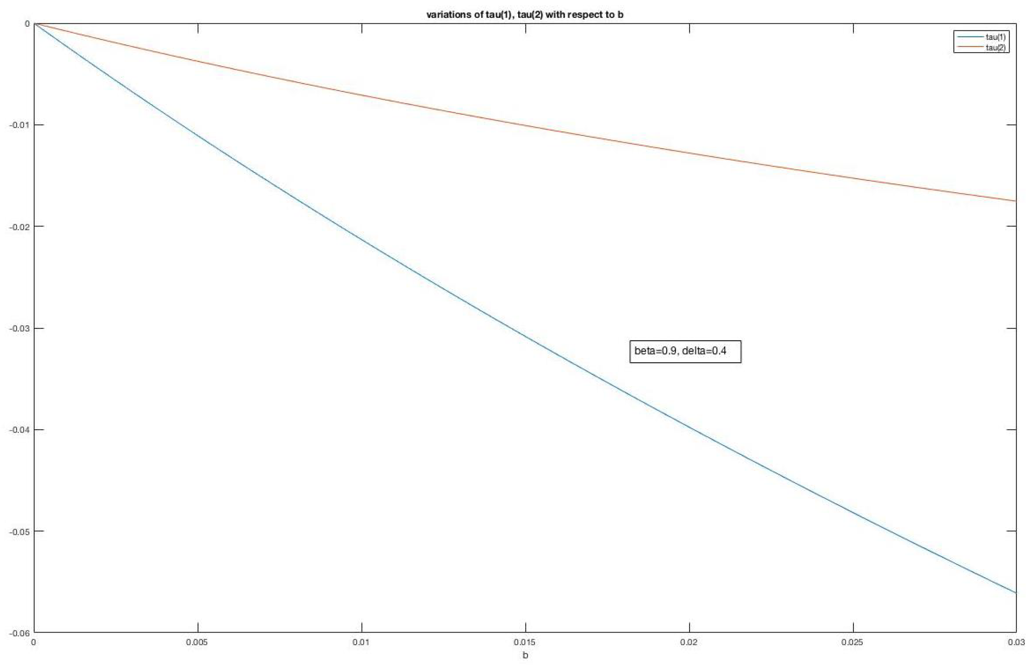
It is not easy to see how the investment rule changes with b, the parameter describing how the equilibrium price depends on the production sent to the market. Figure 1 illustrates that both ${\tau }_1^1$ and ${\tau }_2^1$ decrease with b (the simulations are robust to change in $\delta$ and $\beta$). The larger $b,$ is, the more negative the effect of an increase in $K_1$ or $K_2$ on the output price. This makes investment less profitable, which is reflected by ${\tau }_1^1$ and ${\tau }_2^1$ being decreasing in b.

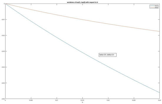
Figure 1. Effects of change of b on ${\tau }_1^1$ and ${\tau }_2^1$, where tau(1) and tau(2) denote, respectively, ${\tau }_1^1$ and ${\tau }_2^1$.

Interestingly, we see that ${\tau }_1^1$ is more negative than ${\tau }_2^2$. This is because the negative effect of $K_2$ on $I_2$ is just caused by the fact that if $K_2$ is larger the output price is lower, which negatively affects the profitability of investment. In the work of Dawid et al. [19], this is called the size effect, and, similarly to $K_2$, this effect also holds for $K_1$. In addition to this effect, a larger value of $K_1$ also raises the cannibalization effect of investment. The cannibalization effect says that investing raises capital stock and then a decrease in the output price makes the profitability lower, because the output price decrease is multiplied by a larger capital stock. So, we conclude that the negative value of ${\tau }_2$ is caused by just the size effect, while the larger negative value (in absolute terms) of ${\tau }_1$ is caused by the sum of the size and the cannibalization effect.

Up to now, we have only presented necessary conditions for the existence of a feedback Nash equilibrium. We now give a sufficient condition for the existence of feedback Nash equilibria.

4.2.1. Existence and Properties of Symmetric Feedback Nash Equilibria

We first address the existence of completely symmetric equilibria when firms give the same relative weights to their environmental objective—that is, ${\tau }_3^1={\tau }_3^2$, and we have

Proposition 2.

Assume that b is small enough. For any pair $({\lambda }_2,{\gamma }_2)$ of relative weights given by the two firms to their environmental objectives, satisfying $0\le {\lambda }_2={\gamma }_2\le \frac{a(1-\beta \eta )}{\beta }$, there exists a symmetric feedback Nash equilibrium.

Proof. 

Consider the conditions given for a symmetric feedback Nash equilibrium:

$$\left\{\begin{array}{c}{\tau }_1^1=\beta [\left(-2b+(1-\delta ){\tau }_1^1\right)({\tau }_1^1+1-\delta )+\left(-b+(1-\delta ){\tau }_2^1\right){\tau }_2^1+\frac{1}{2}\frac{b{z}_1^2}{z_1\beta \left({\tau }_1^1+1-\delta \right)-1}\hfill \\ +\frac{1}{2}\frac{b{z}_2^2}{z_2\beta \left({\tau }_1^1+1-\delta \right)-1}]\hfill \\ {\tau }_2^1=\beta [\left(-2b+(1-\delta ){\tau }_1^1\right){\tau }_2^1+\left(-b+(1-\delta ){\tau }_2^1\right)({\tau }_1^1+1-\delta )-\frac{b{z}_1^2}{z_1\beta \left({\tau }_1^1+1-\delta \right)-1}\frac{{\tau }_2^1}{2\left|{\tau }_2^1\right|}\hfill \\ +\frac{b{z}_2^2}{z_2\beta \left({\tau }_1^1+1-\delta \right)-1}\frac{{\tau }_2^1}{2\left|{\tau }_2^1\right|}]\hfill \\ {\tau }_3^1=\beta [a+\left(-2b+(1-\delta ){\tau }_1^1\right){\tau }_3^1+\left(-b+(1-\delta ){\tau }_2^1\right){\tau }_3^1-\frac{{\lambda }_2\beta }{1-\beta \eta }+(1-\delta ){\tau }_3^1\hfill \\ +\beta {\tau }_2^1\left[\frac{{\lambda }_2\beta }{(1-\beta \eta )\left(\beta \left({\tau }_1^1+1-\delta \right)-1\right)}+\frac{b{C}^f}{\beta \left({\tau }_1^1+1-\delta \right)-1}-\frac{b{z}_1^2}{z_1\beta \left({\tau }_1^1+1-\delta \right)-1}\frac{C^f(z_2-1)+{\tau }_3^1}{z_2-z_1}+\frac{b{z}_2^2}{z_2\beta \left({\tau }_1^1+1-\delta \right)-1}\frac{C^f(z_1-1)+{\tau }_3^1}{z_2-z_1}\right]]\hfill \end{array}\right.$$

We have ${\tau }_2^1<0$. So, from Equations (65) and (66), we have $z_1={\tau }_1^1+{\tau }_2^1+(1-\delta )$ and $z_2={\tau }_1^1-{\tau }_2^1+(1-\delta )$. Summing the first two lines of the system above, we obtain

$$\begin{array}{cc}\hfill {\tau }_1^1+{\tau }_2^1& =\beta \left[-3b+(1-\delta )({\tau }_1^1+{\tau }_2^1)\right]({\tau }_1^1+{\tau }_2^1+1-\delta )+\frac{\beta b{z}_1^2}{\beta z_1({\tau }_1^1+1-\delta )-1},\hfill \end{array}$$

or, using the definition of $z^1$

$$\begin{array}{cc}\hfill z_1-(1-\delta )& =\beta \left[-3b+(1-\delta )\left(z_1-(1-\delta )\right)\right]z_1+\frac{\beta b{z}_1^2}{\beta z_1({\tau }_1^1+1-\delta )-1}.\hfill \end{array}$$

Set

$$g(z_1)=z_1-(1-\delta )-\beta \left[-3b+(1-\delta )\left(z_1-(1-\delta )\right)\right]z_1-\frac{\beta b{z}_1^2}{\beta z_1({\tau }_1^1+1-\delta )-1}.$$

Observe that $g(0)=-(1-\delta )<0$. Let us show that $g(1)>0$. We have

$$\begin{array}{cc}\hfill g(1)& =\delta -\beta \left[-3b+(1-\delta )\delta \right]-\frac{\beta b}{\beta ({\tau }_1^1+1-\delta )-1}\hfill \\ \hfill & =3b\beta +\delta (1-\beta (1-\delta ))-\frac{\beta b}{\beta ({\tau }_1^1+1-\delta )-1}>0\hfill \end{array}$$

since $0\le {\tau }_1^1+(1-\delta )\le 1$ and $0<\beta <1$. So, there exists $z_1\in [0,1]$ such that $g(z_1)=0$

Now subtracting the second line from the first one of the system of equations, we obtain

$$\begin{array}{cc}\hfill {\tau }_1^1-{\tau }_2^1& =\beta \left[-2b+(1-\delta ){\tau }_1^1\right]({\tau }_1^1-{\tau }_2^1+1-\delta )\hfill \\ \hfill & +\beta \left[-b+(1-\delta ){\tau }_2^1\right](-{\tau }_1^1+{\tau }_2^1-(1-\delta ))+\frac{\beta b{z}_2^2}{\beta z_2({\tau }_1^1+1-\delta )-1},\hfill \end{array}$$

or

$$\begin{array}{cc}\hfill {\tau }_1^1-{\tau }_2^1& =\beta \left[(-b+(1-\delta )({\tau }_1^1-{\tau }_2^1)\right]({\tau }_1^1-{\tau }_2^1+1-\delta )\hfill \\ \hfill & +\frac{\beta b{z}_2^2}{\beta z_2({\tau }_1^1+1-\delta )-1},\hfill \end{array}$$

Using the definition of $z_2$ in the equation above we obtain

$$\begin{array}{cc}\hfill z_2-(1-\delta )& =\beta \left[-b+(1-\delta )(z_2-(1-\delta ))\right]z_2+\frac{\beta b{z}_2^2}{\beta z_2({\tau }_1^1+1-\delta )-1}.\hfill \end{array}$$

Set

$$h(z_2)=z_2-(1-\delta )-\beta \left[-b+(1-\delta )(z_2-(1-\delta ))\right]z_2-\frac{\beta b{z}_2^2}{\beta z_2({\tau }_1^1+1-\delta )-1}.$$

We have $h(0)=-(1-\delta )<0$. Let us now show that $h(1)>0$. Moreover,

$$\begin{array}{cc}\hfill h(1)& =\delta -\beta \left[-b+(1-\delta )\delta \right]-\frac{\beta b}{\beta ({\tau }_1^1+1-\delta )-1}\hfill \\ \hfill & =\beta b+{\delta }^2-\frac{\beta b}{\beta ({\tau }_1^1+1-\delta )-1}>0\hfill \end{array}$$

since $0\le {\tau }_1^1+(1-\delta )\le 1$ and $0<\beta <1$. So there exists $z_2\in [0,1]$ such that $h(z_2)=0$.

Consider now the function F defined on $[-(1-\delta ),\delta ]$ by

$$F({\tau }_1^1)={\tau }_1^1-\beta [\left(-2b+(1-\delta ){\tau }_1^1\right)({\tau }_1^1+1-\delta )+\left(-b+(1-\delta ){\tau }_2^1({\tau }_1^1)\right){\tau }_2^1({\tau }_1^1)+\frac{1}{2}\frac{b{(z_1({\tau }_1^1))}^2}{z_1({\tau }_1^1)\beta \left({\tau }_1^1+1-\delta \right)-1}$$

$$+\frac{1}{2}\frac{b{(z_2({\tau }_1^1))}^2}{z_2({\tau }_1^1)\beta \left({\tau }_1^1+1-\delta \right)-1}].$$

Clearly, F is continuous on $[-(1-\delta ),\delta ]$. Using $0\le z_1={\tau }_1^1-\left|{\tau }_2^1\right|+1-\delta \le 1$ and $0\le z_2={\tau }_1^1+\left|{\tau }_2^1\right|+1-\delta \le 1$, we see that when ${\tau }_1^1=-(1-\delta )$, then ${\tau }_2^1(-(1-\delta ))=z_1(-(1-\delta ))=0,z_2(-(1-\delta ))=0$. Thus, $F(-(1-\delta ))=-(1-\delta )<0$.

When ${\tau }_1^1=\delta$, then reasoning as above we have ${\tau }_2^1(\delta )=0,z_1(\delta )=1,z_2(\delta )=1$. Then, $F(\delta )=\delta -\beta \left[(-2b+(1-\delta )\delta +\frac{b}{\beta -1}\frac{1}{2}+\frac{b}{\beta -1}\frac{1}{2}\right]=\delta (1-\beta (1-\delta ))+2b\beta -\beta \frac{b}{\beta -1}>0$. Hence, there exists ${\tau }_1^1\in [-(1-\delta ),\delta ]$ such that $F({\tau }_1^1)=0$. It is now important to obtain ${\tau }_2^1$ as $\left|{\tau }_2^1\right|={\tau }_1^1+1-\delta -z_1$.

Therefore, we have shown the existence of ${\tau }_1^1$, ${\tau }_2^1$, $z_1$, $z_2$ that satisfy the two equations that must hold in an equilibrium.

Finally, we can use the last equation to obtain an expression for ${\tau }_3^1$ (${\tau }_3^2={\tau }_3^1$ in a completely symmetric equilibrium). However, first notice using the definitions of $C^f$, namely Equation (67) and $z_1$, and noting that ${\tilde{C}}^f$ is defined in a similar way as $C^f$, that we have in a completely symmetric equilibrium

$$\begin{array}{c}\hfill {\tilde{C}}^f=C^f=\frac{-{\tau }_3^1({\tau }_1^1-\delta -{\tau }_2^1)}{({\tau }_1^1-\delta -{\tau }_2^1)({\tau }_1^1-\delta +{\tau }_2^1)}=-\frac{{\tau }_3^1}{({\tau }_1^1-\delta +{\tau }_2^1)}=-\frac{{\tau }_3^1}{z_1-1}=\frac{{\tau }_3^1}{1-z_1}>0.\end{array}$$

(73)

Building on this observation, we can use the definition of ${\tau }_3^1$ to obtain

$$\begin{array}{c}{\tau }_3^1=\beta [a+\left(-2b+(1-\delta ){\tau }_1^1\right){\tau }_3^1+\left(-b+(1-\delta ){\tau }_2^1\right){\tau }_3^1-\frac{{\lambda }_2\beta }{1-\beta \eta }+(1-\delta ){\tau }_3^1\hfill \\ +\beta {\tau }_2^1\left[\frac{{\lambda }_2\beta }{(1-\beta \eta )\left(\beta \left({\tau }_1^1+1-\delta \right)-1\right)}+\frac{b{C}^f}{\beta \left({\tau }_1^1+1-\delta \right)-1}-\frac{b{z}_1^2}{z_1\beta \left({\tau }_1^1+1-\delta \right)-1}\frac{C^f(z_2-1)+{\tau }_3^1}{z_2-z_1}+\frac{b{z}_2^2}{z_2\beta \left({\tau }_1^1+1-\delta \right)-1}\frac{C^f(z_1-1)+{\tau }_3^1}{z_2-z_1}\right]].\hfill \end{array}$$

Notice that $C^f(z_1-1)+{\tau }_3^1=0$ and $\frac{C^f(z_2-1)+{\tau }_3^1}{z_2-z_1}=C^f$. Using the equation above, we then obtain

$$\begin{array}{c}\hfill {\tau }_3^1=\frac{\beta \left[a-\frac{{\lambda }_2\beta }{1-\beta \eta }+\beta {\tau }_2^1\frac{{\lambda }_2\beta }{(1-\beta \eta )\left(\beta \left({\tau }_1^1+1-\delta \right)-1\right)}\right]}{S+T}\end{array}$$

(74)

where

$$\begin{array}{cc}\hfill S& =1-\beta \left[\left(-2b+(1-\delta ){\tau }_1^1\right)+(1-\delta )+\left(-b+(1-\delta ){\tau }_2^1\right)\right]\hfill \end{array}$$

(75)

$$\begin{array}{cc}\hfill & =3\beta b+1-\beta (1-\delta )({\tau }_1^1+{\tau }_2^1+1)\hfill \end{array}$$

(76)

$$\begin{array}{cc}\hfill T& =\beta {\tau }_2^1\frac{1}{z_1-1}\left[\frac{b}{\beta \left({\tau }_1^1+1-\delta \right)-1}-\frac{b{z}_1^2}{z_1\beta \left({\tau }_1^1+1-\delta \right)-1}\right].\hfill \end{array}$$

(77)

In particular, if (as in Reynolds, 1987) ${\lambda }_2={\gamma }_2=0$ we have

$$\begin{array}{c}\hfill {\tau }_3^1=\frac{\beta a}{S+T}.\end{array}$$

(78)

We want $S+T>0$ to have ${\tau }_3^1>0$, otherwise, firm i’s capital stock cannot always be non-negative.

Observe that S is positive since $z_1<1<1/(\beta (1-\delta ))-\delta =\frac{1-\beta \delta +\beta {\delta }^2}{\beta -\beta \delta }$ Now, let us turn to T. Recall that $z_1-1<0$. Moreover, $\frac{b}{\beta \left({\tau }_1^1+1-\delta \right)-1}-\frac{b{z}_1^2}{z_1\beta \left({\tau }_1^1+1-\delta \right)-1}<0$ since $\frac{b{z}_1^2}{z_1\beta \left({\tau }_1^1+1-\delta \right)-1}$ is decreasing with $z_1$ (knowing that ${\tau }_1^1<\frac{1}{\beta }-(1-\delta )$). (In fact, when $z_1=0$, $\frac{b}{\beta \left({\tau }_1^1+1-\delta \right)-1}-\frac{b{z}_1^2}{z_1\beta \left({\tau }_1^1+1-\delta \right)-1}<0$, when $z_1=1$, this expression equals 0). So

$${\beta }^2{\tau }_2^1\frac{1}{({\tau }_1^1-\delta +{\tau }_2^1)}(\frac{b}{(\beta \left({\tau }_1^1+1-\delta \right)-1)}-\frac{b{z}_1^2}{(z_1\beta \left({\tau }_1^1+1-\delta \right)-1)})<0.$$

Now, we notice that $S+T>0$ is always true when $b=0$. So, ${\tau }_3^1>0$ if b is small enough and ${\lambda }_2={\gamma }_2=0$.

If ${\lambda }_2={\gamma }_2$ but are different from zero then sufficient conditions to have ${\tau }_3^1>0$ under the hypotheses of the proposition are that b is small enough and $0\le {\lambda }_2\le \frac{a(1-\beta \eta )}{\beta }$. □

Proposition 2 extends the result of Reynolds [10] by taking into account firms’ environmental concerns. The next proposition shows precisely how firms’ investment rules change with the common environmental concern (${\lambda }_2$) in the completely symmetric case.

Proposition 3.

Suppose that the assumptions of Proposition 2 hold. Then, each firm’s investment rule is a decreasing function of their environmental concern.

Proof. 

In the completely symmetric case, the constant term of both firms’ investment rules is given by Equation (74)

$$\begin{array}{c}\hfill {\tau }_3^1=\frac{\beta \left[a-\frac{{\lambda }_2\beta }{1-\beta \eta }+\beta {\tau }_2^1\frac{{\lambda }_2\beta }{(1-\beta \eta )\left(\beta \left({\tau }_1^1+1-\delta \right)-1\right)}\right]}{S+T}.\end{array}$$

Under the assumptions of Proposition 2, the denominator $S+T$ is positive. We have

$$\begin{array}{c}\hfill \frac{\partial {\tau }_3^1}{\partial {\lambda }_2}=-\frac{\beta }{(S+T)(1-\beta \eta )}\frac{-1+\beta z_2}{\beta \left({\tau }_1^1+1-\delta \right)-1}.\end{array}$$

The result follows since the second fraction in the expression above is positive. □

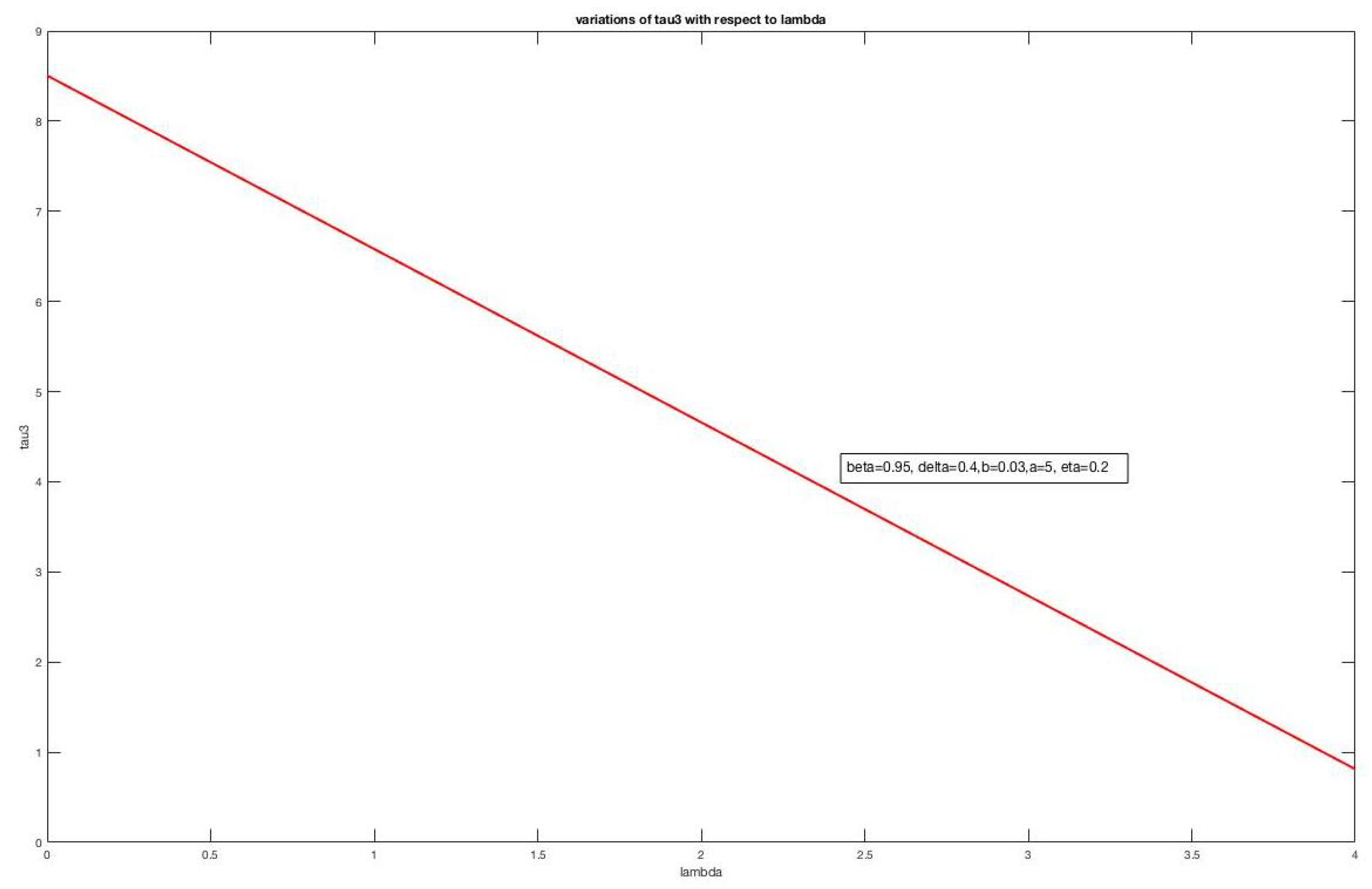
Recall that only the constant terms in the investments rule depend on the relative weights given to the environmental objectives. The proposition states that these constant terms decrease when firms become more environmentally concerned. This proposition is somewhat expected, and it is similar to what we found in the open-loop case. It is illustrated in Figure 2.

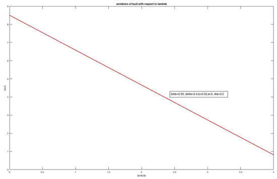
Figure 2. ${\tau }_3^1={\tau }_3^2$ depending on ${\lambda }_2={\gamma }_2$, where tau3 denotes ${\tau }_3^1={\tau }_3^2$.

4.2.2. Existence and Properties of Partially Symmetric Equilibria

Here, we extend the previous section by allowing for the environmental appreciation parameters to be different, i.e., ${\lambda }_2\ne {\gamma }_2$. We obtain the following results.

Proposition 4.

The difference ${\tau }_3^1-{\tau }_3^2$ is a decreasing function of ${\lambda }_2$ and an increasing function of ${\gamma }_2$.

Proof. 

Using the expression of ${\tau }_3^1$ given in Lemma 3, we know that:

$$\begin{array}{c}{\tau }_3^1=\beta \left[a+\left(-2b+(1-\delta ){\tau }_1^1\right){\tau }_3^1+\left(-b+(1-\delta ){\tau }_2^1\right){\tau }_3^2-\frac{{\lambda }_2\beta }{1-\beta \eta }+(1-\delta ){\tau }_3^1\right.\hfill \\ \beta {\tau }_1^2\left[\frac{{\lambda }_2\beta }{(1-\beta \eta )\left(\beta \left({\tau }_2^2+1-\delta \right)-1\right)}+\frac{b{C}^f}{\beta \left({\tau }_2^2+1-\delta \right)-1}-\frac{b{z}_1^2}{z_1\beta \left({\tau }_2^2+1-\delta \right)-1}\frac{C^f(z_2-1)+{\tau }_3^1}{z_2-z_1}\right.\\ \hfill \left.\left.+\frac{b{z}_2^2}{z_2\beta \left({\tau }_2^2+1-\delta \right)-1}\frac{C^f(z_1-1)+{\tau }_3^1}{z_2-z_1}\right]\right]\end{array}$$

(79)

However, ${\tau }_2^2={\tau }_1^1$. Thus,

$$\begin{array}{c}{\tau }_3^1=\beta \left[a+\left(-2b+(1-\delta ){\tau }_1^1\right){\tau }_3^1+\left(-b+(1-\delta ){\tau }_2^1\right){\tau }_3^2-\frac{{\lambda }_2\beta }{1-\beta \eta }+(1-\delta ){\tau }_3^1\right.\hfill \\ \beta {\tau }_1^2\left[\frac{{\lambda }_2\beta }{(1-\beta \eta )\left(\beta \left({\tau }_1^1+1-\delta \right)-1\right)}+\frac{b{C}^f}{\beta \left({\tau }_1^1+1-\delta \right)-1}-\frac{b{z}_1^2}{z_1\beta \left({\tau }_1^1+1-\delta \right)-1}\frac{C^f(z_2-1)+{\tau }_3^1}{z_2-z_1}\right.\\ \hfill \left.\left.+\frac{b{z}_2^2}{z_2\beta \left({\tau }_1^1+1-\delta \right)-1}\frac{C^f(z_1-1)+{\tau }_3^1}{z_2-z_1}\right]\right]\end{array}$$

(80)

By considering symmetry, we have (with ${\tau }_2^1={\tau }_1^2$)

$$\begin{array}{c}{\tau }_3^2=\beta \left[a+\left(-2b+(1-\delta ){\tau }_1^1\right){\tau }_3^2+\left(-b+(1-\delta ){\tau }_2^1\right){\tau }_3^1-\frac{{\gamma }_2\beta }{1-\beta \eta }+(1-\delta ){\tau }_3^2\right.\hfill \\ \beta {\tau }_1^2\left[\frac{{\gamma }_2\beta }{(1-\beta \eta )\left(\beta \left({\tau }_1^1+1-\delta \right)-1\right)}+\frac{b{\tilde{C}}^f}{\beta \left({\tau }_1^1+1-\delta \right)-1}-\frac{b{z}_1^2}{z_1\beta \left({\tau }_1^1+1-\delta \right)-1}\frac{{\tilde{C}}^f(z_2-1)+{\tau }_3^2}{z_2-z_1}\right.\\ \hfill \left.\left.+\frac{b{z}_2^2}{z_2\beta \left({\tau }_1^1+1-\delta \right)-1}\frac{{\tilde{C}}^f(z_1-1)+{\tau }_3^2}{z_2-z_1}\right]\right]\end{array}$$

(81)

Thus,

$$\begin{array}{c}{\tau }_3^1-{\tau }_3^2=\beta \left[\left(-2b+(1-\delta ){\tau }_1^1\right)({\tau }_3^1-{\tau }_3^2)+\left(-b+(1-\delta ){\tau }_2^1\right)({\tau }_3^2-{\tau }_3^1)-\frac{\beta ({\lambda }_2-{\gamma }_2)}{1-\beta \eta }\right.\hfill \\ +(1-\delta )({\tau }_3^1-{\tau }_3^2)\\ \beta {\tau }_1^2\left[\frac{\beta ({\lambda }_2-{\gamma }_2)}{(1-\beta \eta )\left(\beta \left({\tau }_1^1+1-\delta \right)-1\right)}+\frac{b(C^f-{\tilde{C}}^f)}{\beta \left({\tau }_1^1+1-\delta \right)-1}\right.\\ -\frac{b{z}_1^2}{z_1\beta \left({\tau }_1^1+1-\delta \right)-1}\frac{(C^f-{\tilde{C}}^f)(z_2-1)+{\tau }_3^1-{\tau }_3^2}{z_2-z_1}\\ \hfill \left.\left.+\frac{b{z}_2^2}{z_2\beta \left({\tau }_1^1+1-\delta \right)-1}\frac{(C^f-{\tilde{C}}^f)(z_1-1)+{\tau }_3^1-{\tau }_3^2}{z_2-z_1}\right]\right]\end{array}$$

(82)

Now, we have

$$\begin{array}{cc}\hfill C^f& =\frac{-{\tau }_3^1({\tau }_1^1-\delta )+{\tau }_2^1{\tau }_3^2}{-{\tau }_2^1{\tau }_2^1+({\tau }_1^1-\delta )({\tau }_1^1-\delta )}>0.\hfill \end{array}$$

(83)

$$\begin{array}{cc}\hfill {\tilde{C}}^f& =\frac{-{\tau }_3^2({\tau }_1^1-\delta )+{\tau }_2^1{\tau }_3^1}{-{\tau }_2^1{\tau }_2^1+({\tau }_1^1-\delta )({\tau }_1^1-\delta )}>0.\hfill \end{array}$$

(84)

and thus

$$\begin{array}{cc}\hfill C^f-{\tilde{C}}^f& =\frac{-({\tau }_3^1-{\tau }_3^2)({\tau }_1^1-\delta )+{\tau }_2^1({\tau }_3^2-{\tau }_3^1)}{-{({\tau }_2^1)}^2+{({\tau }_1^1-\delta )}^2}\hfill \end{array}$$

(85)

$$\begin{array}{cc}\hfill & \frac{-({\tau }_3^1-{\tau }_3^2)({\tau }_1^1+{\tau }_2^1-\delta )}{-{({\tau }_2^1)}^2+{({\tau }_1^1-\delta )}^2}\hfill \end{array}$$

(86)

$$\begin{array}{cc}\hfill & =\frac{-({\tau }_3^1-{\tau }_3^2)}{{\tau }_1^1-{\tau }_1^2-\delta }\hfill \end{array}$$

(87)

We also have

$$\begin{array}{cc}\hfill (C^f-{\tilde{C}}^f)(z_2-1)+{\tau }_3^1-{\tau }_3^2& =\frac{-({\tau }_3^1-{\tau }_3^2)}{{\tau }_1^1-{\tau }_1^2-\delta }({\tau }_1^1-{\tau }_2^1-\delta )+{\tau }_3^1-{\tau }_3^2\hfill \end{array}$$

(88)

$$\begin{array}{cc}\hfill & =0,\hfill \end{array}$$

(89)

and

$$\begin{array}{cc}\hfill (C^f-{\tilde{C}}^f)(z_1-1)+{\tau }_3^1-{\tau }_3^2& =\frac{-({\tau }_3^1-{\tau }_3^2)}{{\tau }_1^1-{\tau }_1^2-\delta }({\tau }_1^1+{\tau }_1^2-\delta )+{\tau }_3^1-{\tau }_3^2\hfill \end{array}$$

(90)

$$\begin{array}{cc}\hfill & =({\tau }_3^1-{\tau }_3^2)\frac{-({\tau }_1^1+{\tau }_1^2-\delta )+{\tau }_1^1-{\tau }_1^2-\delta }{{\tau }_1^1-{\tau }_1^2-\delta }\hfill \end{array}$$

(91)

$$\begin{array}{cc}\hfill & =({\tau }_3^1-{\tau }_3^2)\frac{-({\tau }_1^1+{\tau }_1^2-\delta )+{\tau }_1^1-{\tau }_1^2-\delta }{{\tau }_1^1-{\tau }_1^2-\delta }\hfill \end{array}$$

(92)

$$\begin{array}{cc}\hfill & =({\tau }_3^1-{\tau }_3^2)\frac{-2{\tau }_2^1}{{\tau }_1^1-{\tau }_1^2-\delta }.\hfill \end{array}$$

(93)

So, using $z_2-z_1=-2{\tau }_2^1$, we obtain

$$\begin{array}{c}{\tau }_3^1-{\tau }_3^2=\beta \left[\left(-2b+(1-\delta ){\tau }_1^1\right)({\tau }_3^1-{\tau }_3^2)+\left(-b+(1-\delta ){\tau }_2^1\right)({\tau }_3^2-{\tau }_3^1)-\frac{\beta ({\lambda }_2-{\gamma }_2)}{1-\beta \eta }\right.\hfill \\ +(1-\delta )({\tau }_3^1-{\tau }_3^2)\\ \beta {\tau }_1^2\left[\frac{\beta ({\lambda }_2-{\gamma }_2)}{(1-\beta \eta )\left(\beta \left({\tau }_1^1+1-\delta \right)-1\right)}+\frac{b}{\beta \left({\tau }_1^1+1-\delta \right)-1}\frac{-({\tau }_3^1-{\tau }_3^2)}{{\tau }_1^1-{\tau }_1^2-\delta }\right.\\ \hfill \left.\left.+\frac{b{z}_2^2}{z_2\beta \left({\tau }_1^1+1-\delta \right)-1}({\tau }_3^1-{\tau }_3^2)\frac{1}{{\tau }_1^1-{\tau }_1^2-\delta }.\right]\right]\end{array}$$

(94)

Hence,

$$\begin{array}{c}({\tau }_3^1-{\tau }_3^2)\left(1-\beta \left(\left(-2b+(1-\delta ){\tau }_1^1\right)-\left(-b+(1-\delta ){\tau }_2^1\right)+(1-\delta )-\beta \frac{{\tau }_1^2}{{\tau }_1^1-{\tau }_1^2-\delta }\left(\frac{b}{\beta \left({\tau }_1^1+1-\delta \right)-1}\right.\right.\right.\hfill \\ \left.\left.\left.-\frac{b{z}_2^2}{z_2\beta \left({\tau }_1^1+1-\delta \right)-1}\right)\right)\right)\\ \hfill =\beta \left[-\frac{\beta ({\lambda }_2-{\gamma }_2)}{1-\beta \eta }+\beta {\tau }_1^2\left[\frac{\beta ({\lambda }_2-{\gamma }_2)}{(1-\beta \eta )\left(\beta \left({\tau }_1^1+1-\delta \right)-1\right)}\right]\right]\end{array}$$

(95)

Regarding the right-hand side, observe that

$$\begin{array}{c}-\frac{\beta ({\lambda }_2-{\gamma }_2)}{1-\beta \eta }+\beta {\tau }_1^2\left[\frac{\beta ({\lambda }_2-{\gamma }_2)}{(1-\beta \eta )\left(\beta \left({\tau }_1^1+1-\delta \right)-1\right)}\right]\hfill \\ =\frac{\beta ({\lambda }_2-{\gamma }_2)}{1-\beta \eta }\left(-1+\frac{\beta {\tau }_2^1}{\beta \left({\tau }_1^1+1-\delta \right)-1}\right)\\ =\frac{\beta ({\lambda }_2-{\gamma }_2)}{1-\beta \eta }\left(\frac{\beta {\tau }_2^1-(\beta ({\tau }_1^1+1-\delta )-1)}{\beta \left({\tau }_1^1+1-\delta \right)-1}\right)\\ =\frac{\beta ({\lambda }_2-{\gamma }_2)}{1-\beta \eta }\left(\frac{\beta ({\tau }_2^1-{\tau }_1^1-1+\delta )+1}{\beta \left({\tau }_1^1+1-\delta \right)-1}\right)\\ =\frac{\beta ({\lambda }_2-{\gamma }_2)}{1-\beta \eta }\left(\frac{-\beta z_2+1}{\beta \left({\tau }_1^1+1-\delta \right)-1}\right)\\ \hfill =-\frac{\beta ({\lambda }_2-{\gamma }_2)}{1-\beta \eta }\left(\frac{1-\beta z_2}{1-\beta \left({\tau }_1^1+1-\delta \right)}\right)\end{array}$$

(96)

Thus,

$$\begin{array}{c}({\tau }_3^1-{\tau }_3^2)\left(1-\beta \left(\left(-2b+(1-\delta ){\tau }_1^1\right)-\left(-b+(1-\delta ){\tau }_2^1\right)+(1-\delta )-\beta \frac{b{\tau }_1^2}{{\tau }_1^1-{\tau }_1^2-\delta }\left(\frac{1}{\beta \left({\tau }_1^1+1-\delta \right)-1}\right.\right.\right.\hfill \\ \left.\left.\left.-\frac{z_2^2}{z_2\beta \left({\tau }_1^1+1-\delta \right)-1}\right)\right)\right)\\ \hfill =-\beta \frac{\beta ({\lambda }_2-{\gamma }_2)}{1-\beta \eta }\left(\frac{1-\beta z_2}{1-\beta \left({\tau }_1^1+1-\delta \right)}\right)\end{array}$$

(97)

Notice that

$$\begin{array}{c}\hfill 1-\beta \left(\left(-2b+(1-\delta ){\tau }_1^1\right)-\left(-b+(1-\delta ){\tau }_2^1\right)+(1-\delta )\right)=\beta b+1-\beta (1-\delta )z_2>0.\end{array}$$

(98)

Moreover,

$$\begin{array}{c}\frac{1}{\beta \left({\tau }_1^1+1-\delta \right)-1}-\frac{z_2^2}{z_2\beta \left({\tau }_1^1+1-\delta \right)-1}=\hfill \\ \hfill \frac{(1-z_2)\left(\beta z_2({\tau }_1^1+1-\delta )-(1+z_2)\right)}{\left(\beta ({\tau }_1^1+1-\delta )-1\right)\left(z_2\beta ({\tau }_1^1+1-\delta )-1\right)}<0.\end{array}$$

(99)

Hence,

$$\begin{array}{cc}\hfill {\tau }_3^1-{\tau }_3^2& =\frac{-\beta \frac{\beta ({\lambda }_2-{\gamma }_2)}{1-\beta \eta }\left(\frac{1-\beta z_2}{1-\beta \left({\tau }_1^1+1-\delta \right)}\right)}{\beta b+1-\beta (1-\delta )z_2+{\beta }^2\frac{b{\tau }_1^2}{z^2-1}\frac{(1-z_2)\left(\beta z_2({\tau }_1^1+1-\delta )-(1+z_2)\right)}{\left(\beta ({\tau }_1^1+1-\delta )-1\right)\left(z_2\beta ({\tau }_1^1+1-\delta )-1\right)}}\hfill \end{array}$$

(100)

$$\begin{array}{cc}\hfill & =\frac{-\beta \frac{\beta ({\lambda }_2-{\gamma }_2)}{1-\beta \eta }\left(\frac{1-\beta z_2}{1-\beta \left({\tau }_1^1+1-\delta \right)}\right)}{\beta b+1-\beta (1-\delta )z_2-b\frac{{\beta }^2{\tau }_1^2}{1+z_2}\frac{\beta z_2({\tau }_1^1+1-\delta )-(1+z_2)}{\left(\beta ({\tau }_1^1+1-\delta )-1\right)\left(z_2\beta ({\tau }_1^1+1-\delta )-1\right)}}.\hfill \end{array}$$

(101)

As for the denominator, its sign is positive if (consider the factor of b):

$$\begin{array}{c}\hfill 1-\beta {\tau }_1^2\frac{\beta z_2({\tau }_1^1+1-\delta )-(1+z_2)}{\left(\beta ({\tau }_1^1+1-\delta )-1\right)\left(z_2\beta ({\tau }_1^1+1-\delta )-1\right)}.\end{array}$$

(102)

Observe that

$$\begin{array}{cc}\hfill \left(\beta ({\tau }_1^1+1-\delta )-1\right)\left(z_2\beta ({\tau }_1^1+1-\delta )-1\right)-\beta {\tau }_2^1\left(\beta z_2({\tau }_1^1+1-\delta )-(1+z_2)\right)& \end{array}$$

(103)

$$\begin{array}{cc}\hfill =\left(z_2\beta ({\tau }_1^1+1-\delta )-1\right)\left(\beta ({\tau }_1^1+1-\delta )-1-\beta {\tau }_1^2\right)+\beta {\tau }_2^1(1-z_2)& \end{array}$$

(104)

$$\begin{array}{cc}\hfill =\left(z_2\beta ({\tau }_1^1+1-\delta )-1\right)\left(\beta ({\tau }_1^1-{\tau }_2^1+1-\delta )-1\right)+\beta {\tau }_2^1(1-z_2)& \end{array}$$

(105)

$$\begin{array}{cc}\hfill =\left(z_2\beta ({\tau }_1^1+1-\delta )-1\right)\left(\beta z_2-1\right)+\beta {\tau }_2^1(1-z_2)& \end{array}$$

(106)

$$\begin{array}{cc}\hfill \ge (1-z_2)\left(1-z_2\beta ({\tau }_1^1+1-\delta )+\beta {\tau }_2^1)\right)& \end{array}$$

(107)

$$\begin{array}{cc}\hfill \ge (1-z_2)\left(1-\beta ({\tau }_1^1+1-\delta +{\tau }_2^1)\right)& \end{array}$$

(108)

$$\begin{array}{c}\hfill =(1-z_2)(1-\beta z_2)>0.\end{array}$$

(109)

Therefore, ${\tau }_3^1-{\tau }_3^2$ decreases with ${\lambda }_2$ and increases with ${\gamma }_2$. □

Proposition 5.

Suppose that b is small enough and that

$$\begin{array}{cc}\hfill {\lambda }_2& <\frac{a(1-\beta \eta )}{\beta (1+\frac{1-\delta }{2})},\hfill \end{array}$$

(110)

$$\begin{array}{cc}\hfill {\gamma }_2& <\frac{a(1-\beta \eta )}{\beta (1+\frac{1-\delta }{2})}.\hfill \end{array}$$

(111)

Then, there exists a partially symmetric feedback Nash equilibrium.

Proof. 

The existence of ${\tau }_1^1$ and ${\tau }_2^1$ (which are equal to ${\tau }_2^2$ and ${\tau }_1^2$, respectively) can be obtained as in the proof of Proposition 2. We can then use the proof of Proposition 4 to obtain an expression of both ${\tau }_3^1$ and ${\tau }_3^2$. To achieve this we use the fact that

$$\begin{array}{cc}\hfill C^f& =\frac{{\tau }_3^1({\tau }_2^1-{\tau }_1^1+\delta )-{\tau }_2^1({\tau }_3^1-{\tau }_3^2)}{{({\tau }_1^1-\delta )}^2-{({\tau }_2^1)}^2}\hfill \end{array}$$

(112)

$$\begin{array}{cc}\hfill \frac{C^f(z_2-1)+{\tau }_3^1}{z_2-z_1}& =-\frac{{\tau }_3^1}{{\tau }_1^1-\delta +{\tau }_2^1}+\frac{1}{2}\frac{{\tau }_3^1-{\tau }_3^2}{{\tau }_1^1-\delta +{\tau }_2^1}\hfill \end{array}$$

(113)

$$\begin{array}{cc}\hfill & =-\frac{1}{2}\frac{{\tau }_3^1-{\tau }_3^2}{1-z_1}.\hfill \end{array}$$

(114)

$$\begin{array}{cc}\hfill \frac{C^f(z_1-1)+{\tau }_3^1}{z_2-z_1}& =\frac{1}{2}\frac{{\tau }_3^1-{\tau }_3^2}{{\tau }_1^1-\delta -{\tau }_2^1}\hfill \end{array}$$

(115)

$$\begin{array}{cc}\hfill & =-\frac{1}{2}\frac{{\tau }_3^1}{1-z_2}.\hfill \end{array}$$

(116)

Recall that for ${\tau }_3^1$ we have

$$\begin{array}{c}{\tau }_3^1=\beta \left[a+\left(-2b+(1-\delta ){\tau }_1^1\right){\tau }_3^1+\left(-b+(1-\delta ){\tau }_2^1\right)({\tau }_3^2-{\tau }_3^1+{\tau }_3^1)-\frac{{\lambda }_2\beta }{1-\beta \eta }+(1-\delta ){\tau }_3^1\right.\hfill \\ \beta {\tau }_1^2\left[\frac{{\lambda }_2\beta }{(1-\beta \eta )\left(\beta \left({\tau }_1^1+1-\delta \right)-1\right)}+\frac{b{C}^f}{\beta \left({\tau }_1^1+1-\delta \right)-1}-\frac{b{z}_1^2}{z_1\beta \left({\tau }_1^1+1-\delta \right)-1}\frac{C^f(z_2-1)+{\tau }_3^1}{z_2-z_1}\right.\\ \hfill \left.\left.+\frac{b{z}_2^2}{z_2\beta \left({\tau }_1^1+1-\delta \right)-1}\frac{C^f(z_1-1)+{\tau }_3^1}{z_2-z_1}\right]\right]\end{array}$$

(117)

Therefore, we obtain

$$\begin{array}{c}{\tau }_3^1\left[1-\beta \left(\left(-2b+(1-\delta ){\tau }_1^1\right)+\left(-b+(1-\delta ){\tau }_2^1\right)+(1-\delta )\right)\right]\hfill \\ =\beta \left[a-\frac{{\lambda }_2\beta }{1-\beta \eta }+\left(-b+(1-\delta ){\tau }_2^1\right)({\tau }_3^2-{\tau }_3^1)\right.\\ \beta {\tau }_1^2\left[\frac{{\lambda }_2\beta }{(1-\beta \eta )\left(\beta \left({\tau }_1^1+1-\delta \right)-1\right)}+\frac{b}{\beta \left({\tau }_1^1+1-\delta \right)-1}\left(\frac{{\tau }_3^1({\tau }_2^1-{\tau }_1^1+\delta )-{\tau }_2^1({\tau }_3^1-{\tau }_3^2)}{{({\tau }_1^1-\delta )}^2-{({\tau }_2^1)}^2}\right)\right.\\ -\frac{b{z}_1^2}{z_1\beta \left({\tau }_1^1+1-\delta \right)-1}\left(-\frac{{\tau }_3^1}{{\tau }_1^1-\delta +{\tau }_2^1}+\frac{1}{2}\frac{{\tau }_3^1-{\tau }_3^2}{{\tau }_1^1-\delta +{\tau }_2^1}\right)\\ \hfill \left.\left.+\frac{b{z}_2^2}{z_2\beta \left({\tau }_1^1+1-\delta \right)-1}\frac{1}{2}\frac{{\tau }_3^1-{\tau }_3^2}{{\tau }_1^1-\delta -{\tau }_2^1}\right]\right]\end{array}$$

(118)

or

$$\begin{array}{c}{\tau }_3^1\left[1-\beta \left(\left(-2b+(1-\delta ){\tau }_1^1\right)+\left(-b+(1-\delta ){\tau }_2^1\right)+(1-\delta )+\beta {\tau }_2^1\frac{b}{\beta ({\tau }_1^1+1-\delta )-1}\frac{{\tau }_2^1-{\tau }_1^1+\delta }{{({\tau }_1^1-\delta )}^2-{({\tau }_2^1)}^2}\right.\right.\hfill \\ \left.\left.+\beta {\tau }_2^1\frac{b{z}_1^2}{z_1\beta \left({\tau }_1^1+1-\delta \right)-1}\frac{1}{{\tau }_1^1-\delta +{\tau }_2^1}\right)\right]\\ =\beta \left[a-\frac{{\lambda }_2\beta }{1-\beta \eta }+\left(-b+(1-\delta ){\tau }_2^1\right)({\tau }_3^2-{\tau }_3^1)\right.\\ +\beta {\tau }_1^2\left[\frac{{\lambda }_2\beta }{(1-\beta \eta )\left(\beta \left({\tau }_1^1+1-\delta \right)-1\right)}+\frac{b}{\beta \left({\tau }_1^1+1-\delta \right)-1}\frac{-{\tau }_2^1({\tau }_3^1-{\tau }_3^2)}{{({\tau }_1^1-\delta )}^2-{({\tau }_2^1)}^2}\right.\\ -\frac{b{z}_1^2}{z_1\beta \left({\tau }_1^1+1-\delta \right)-1}\frac{1}{2}\frac{{\tau }_3^1-{\tau }_3^2}{{\tau }_1^1-\delta +{\tau }_2^1}\\ \hfill \left.\left.+\frac{b{z}_2^2}{z_2\beta \left({\tau }_1^1+1-\delta \right)-1}\frac{1}{2}\frac{{\tau }_3^1-{\tau }_3^2}{{\tau }_1^1-\delta -{\tau }_2^1}\right]\right]\end{array}$$

(119)

Rearranging, we obtain

$$\begin{array}{c}{\tau }_3^1\left[1-\beta \left(\left(-2b+(1-\delta ){\tau }_1^1\right)+\left(-b+(1-\delta ){\tau }_2^1\right)+(1-\delta )-\beta {\tau }_2^1\frac{b}{1-\beta ({\tau }_1^1+1-\delta )}\frac{1}{1-z_1}\right.\right.\hfill \\ \left.\left.+\beta {\tau }_2^1\frac{b{z}_1^2}{1-z_1\beta \left({\tau }_1^1+1-\delta \right)}\frac{1}{1-z_1}\right)\right]\\ =\beta \left[a-\frac{{\lambda }_2\beta }{1-\beta \eta }-\beta {\tau }_1^2\frac{{\lambda }_2\beta }{(1-\beta \eta )\left(1-\beta \left({\tau }_1^1+1-\delta \right)\right)}\right]\\ +\beta ({\tau }_3^1-{\tau }_3^2)\left[-\left(-b+(1-\delta ){\tau }_2^1\right)\phantom{\frac{1}{\beta \left({\tau }_1^1+1-\delta \right)-1}}\right.\\ +\frac{b\beta {\tau }_1^2}{(1-z_1)(1-z_2)}\left[\frac{1}{1-\beta \left({\tau }_1^1+1-\delta \right)}{\tau }_2^1-\frac{1}{2}\frac{z_1^2(1-z_2)}{1-z_1\beta \left({\tau }_1^1+1-\delta \right)}\right.\\ \hfill \left.\left.+\frac{1}{2}\frac{z_2^2(1-z_1)}{1-z_2\beta \left({\tau }_1^1+1-\delta \right)}\right]\right]\end{array}$$

(120)

Now we have

$$\begin{array}{cc}\hfill \underset{b\to 0}{lim}{\tau }_3^1& =\frac{\beta \left[a-\beta \frac{1-\beta z_2}{1-\beta ({\tau }_1^1+1-\delta )}\left({\lambda }_2-(1-\delta ){\tau }_2^1({\lambda }_2-{\gamma }_2)\right)\right]}{1-\beta (1-\delta )({\tau }_1^1+{\tau }_2^1+1)}\hfill \end{array}$$

(121)

Since ${\lambda }_2$ is upper bounded by $\frac{a(1-\beta \eta )}{\beta (1+\frac{1-\delta }{2})}$, the expression above is positive. Then, it remains so when b is small enough. The same argument applies to ${\tau }_3^2$. □

Proposition 6.

Assume that the assumptions of Proposition 5 holds. Then, ${\tau }_3^1$ is a decreasing function of ${\lambda }_2$ and an increasing function of ${\gamma }_2$ and vice versa for ${\tau }_3^2$.

Proof. 

The assertion is true for ${\tau }_3^1$ when b is small enough (see Equation (121)). □

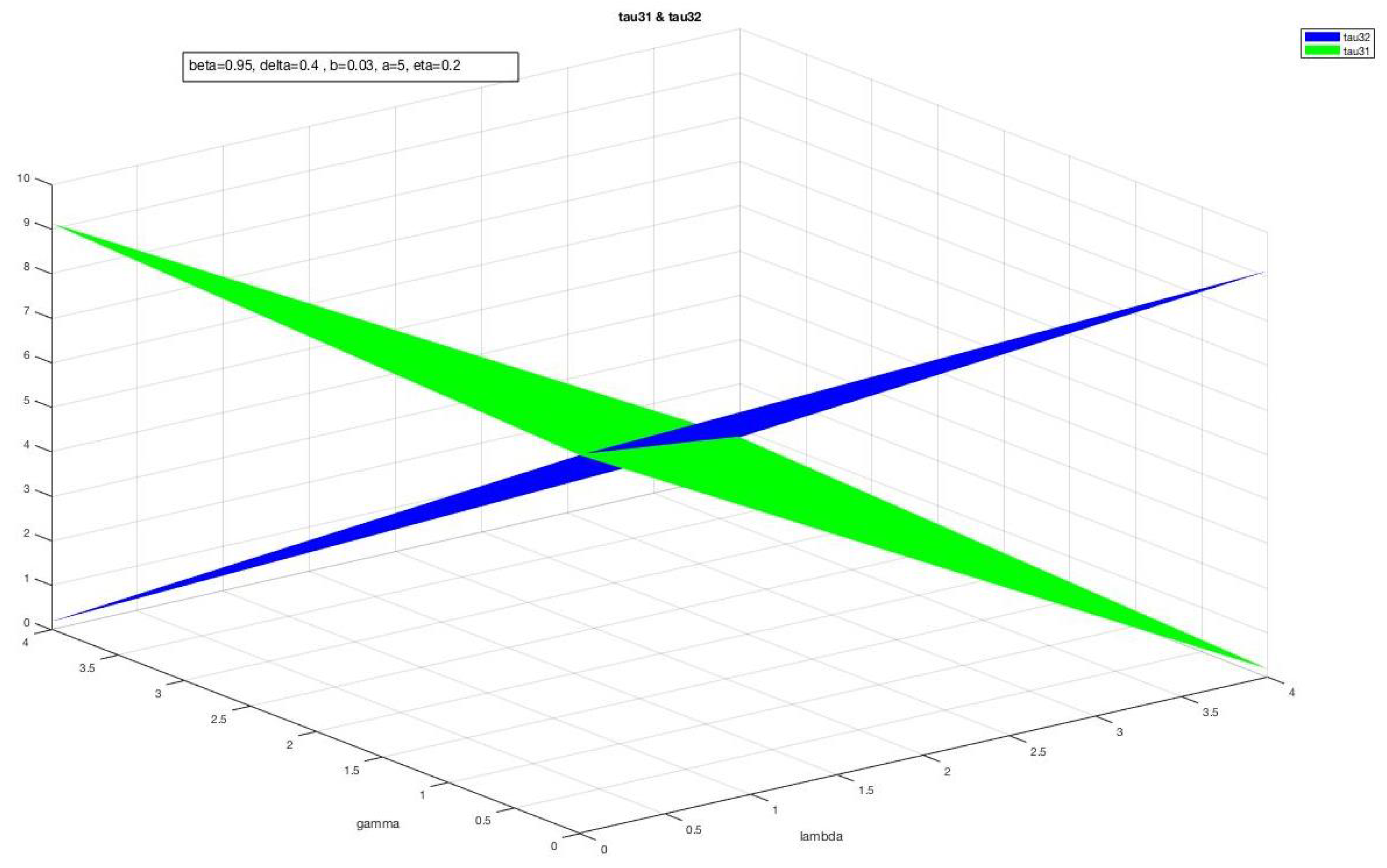
This result generalizes what was seen in the symmetric case and in the open-loop case. Notice that a larger ${\gamma }_2$ reduces the investment rate of firm 2 and thus its capital $K_2$. This increases the output price, which in turn raises the profitability of investment for firm 1. The proposition is illustrated in Figure 3.

Figure 3. ${\tau }_3^1$ and ${\tau }_3^2$ depending on ${\lambda }_2$ and ${\gamma }_2$, where tau31 and tau32 denote, respectively, ${\tau }_3^1$ and ${\tau }_3^2$.

5. Cooperative Equilibrium

There are several ways to define cooperation for multi-objective firms. For instance, one could consider that firms collectively address the problem including all the firms’ objectives. Here, we follow a slightly different road. We suppose that both firms maximize the aggregate sum of their profits, i.e., they behave as a monopoly and minimize the aggregate pollution level. This implies that what matters for them is the effect of the aggregate value $Z_t$ of the capital stock on the aggregate profits and pollution. More formally, we assume that firms solve the following problem

$$\underset{{(I_{it},I_{3-it})}_t}{max}\left\{\sum _{t=0}^{\infty }{\beta }^t\left((a-b{Z}_t)Z_t-\frac{I_{it}^2}{2}-\frac{I_{3-it}^2}{2}\right),-\sum _0^{\infty }{\beta }^t{x}_t\right\}$$

(122)

subject to

$$\begin{array}{cc}\hfill Z_{t+1}& =I_{it}+I_{3-it}+(1-\delta )Z_t,\hfill \end{array}$$

(123)

$$\begin{array}{cc}\hfill x_{t+1}& =\eta x_t+Z_t,Z_0=K_{i0}+K_{3-i0}\mathrm{being}\mathrm{given}.\hfill \end{array}$$

(124)

and the solution is the cooperative equilibrium.

Proposition 7.

For any weight ν given to the environmental objective of the firms that is such that $\nu \frac{\beta }{1-\beta \eta }<a$, there exists a cooperative equilibrium $Z_t=(K_{10}+K_{20}-C^{″})v_1^t+C^{″}$ where

$$\begin{array}{cc}\hfill v_1& =\frac{2(1-\delta )}{\beta \left[{(1-\delta )}^2+4b+1/\beta +\sqrt{{\Delta }^{″}}\right]},\hfill \\ \hfill {\Delta }^{″}& ={\left({(1-\delta )}^2+4b+1/\beta \right)}^2-4{(1-\delta )}^2/\beta ,\hfill \\ \hfill C^{″}& =\frac{2(a-\nu \frac{\beta }{1-\beta \eta })}{\delta (-1+\delta +1/\beta )+4b}.\hfill \end{array}$$

Proof. 

Optimality conditions. Proceeding as in the preceding optimization problem, if a sequence $(I_{1t},I_{2t})$ is solution to problem (122)–(124), then from Theorem 4.2 in the work of Hayek (2018) there exist $\lambda \ge 0,$$\nu \ge 0$, ${({\mu }_t)}_t$ in ${\ell }^1$, ${({\psi }_t)}_t$ in ${\ell }^1$ not all nil, such that any each date, $(I_{1t},I_{2t})$ maximize the following Hamiltonian

$$\begin{array}{cc}\hfill H(I_{1t},I_{2t},Z_t,x_t,\lambda ,\nu ,{\mu }_t,{\psi }_t)& =\lambda {\beta }^t((a-b{Z}_t)Z_t-\frac{I_{1t}^2}{2}-\frac{I_{2t}^2}{2})-\nu {\beta }^t{x}_t\hfill \\ \hfill & +{\mu }_{t+1}\left(\eta x_t+Z_t\right)+{\psi }_{t+1}\left(I_{1t}+I_{2t}+(1-\delta )Z_t\right).\hfill \end{array}$$

The first-order conditions are given by

$$\begin{array}{cc}\hfill 0& =-\lambda {\beta }^t{I}_{1t}+{\psi }_{t+1},\hfill \end{array}$$

(125)

$$\begin{array}{cc}\hfill 0& =-\lambda {\beta }^t{I}_{2t}+{\psi }_{t+1},\hfill \end{array}$$

(126)

$$\begin{array}{cc}\hfill {\psi }_t& =\lambda {\beta }^t\left(a-2b{Z}_t\right)+{\mu }_{t+1}+(1-\delta ){\psi }_{t+1},\hfill \end{array}$$

(127)

$$\begin{array}{cc}\hfill {\mu }_t& =-\nu {\beta }^t+\eta {\mu }_{t+1}.\hfill \end{array}$$

(128)

It holds that $\lambda \ne 0$. Otherwise, we would have ${\psi }_{t+1}=0$ for all t, which in turn would yield ${\mu }_{t+1}=0$ for all t, and thus $\nu =0$, so that all those multipliers would be nil, which is impossible. Then set $\lambda =1$. Notice that we obtain $I_{1t}=I_{2t}=\frac{{\psi }_{t+1}}{{\beta }^t}$. This is because firms’ cost functions are similar. Now by a standard argument, we also obtain

$$\begin{array}{cc}\hfill {\mu }_t& =-\frac{\nu {\beta }^t}{1-\beta \eta }.\hfill \end{array}$$

(129)

Let us now solve the following dynamic system

$$\begin{array}{cc}\hfill {\psi }_t& ={\beta }^t\left(a-2b{Z}_t\right)+(-\frac{\nu {\beta }^{t+1}}{1-\beta \eta })+(1-\delta ){\psi }_{t+1},\hfill \end{array}$$

(130)

$$\begin{array}{cc}\hfill Z_{t+1}& =2\frac{{\psi }_{t+1}}{{\beta }^t}+(1-\delta )Z_t,\hfill \end{array}$$

(131)

$$\begin{array}{cc}\hfill x_{t+1}& =\eta x_t+Z_t.\hfill \end{array}$$

(132)

Setting $\frac{{\psi }_t}{{\beta }^t}={\Psi }_t$ in the system above, we obtain

$$\begin{array}{cc}\hfill {\Psi }_t=& \left(a-2b{Z}_t\right)-\frac{\nu \beta }{1-\beta \eta }+(1-\delta )\beta {\Psi }_{t+1},\hfill \end{array}$$

(133)

$$\begin{array}{cc}\hfill Z_{t+1}& =2\beta {\Psi }_{t+1}+(1-\delta )Z_t.\hfill \end{array}$$

(134)

Using Equation (133) in (134), we obtain

$$\begin{array}{cc}\hfill (1-\delta )Z_{t+2}& -Z_{t+1}\left({(1-\delta )}^2+4b+1/\beta \right)+(1-\delta )Z_t/\beta =2\nu \frac{\beta }{1-\beta \eta }-2a\hfill \end{array}$$

(135)

We have

$$Z_t=w_1{v}_1^t+w_2{v}_2^t+C^{″}$$

where

$$\begin{array}{cc}\hfill v_1& =\frac{{(1-\delta )}^2+4b+1/\beta -\sqrt{{\Delta }^{″}}}{2(1-\delta )},\hfill \end{array}$$

(136)

$$\begin{array}{cc}\hfill v_2& =\frac{{(1-\delta )}^2+4b+1/\beta +\sqrt{{\Delta }^{″}}}{2(1-\delta )},\hfill \end{array}$$

(137)

$$\begin{array}{cc}\hfill {\Delta }^{″}& ={\left({(1-\delta )}^2+4b+1/\beta \right)}^2-4{(1-\delta )}^2/\beta ,\hfill \end{array}$$

(138)

$$\begin{array}{cc}\hfill C^{″}& =\frac{2(a-\nu \frac{\beta }{1-\beta \eta })}{\delta (-1+\delta +1/\beta )+4b}.\hfill \end{array}$$

(139)

Notice that $v_1=\frac{2(1-\delta )}{\beta [{(1-\delta )}^2+4b+1/\beta +\sqrt{{\Delta }^{″}}]}<1$, and as $v_1{v}_2=1/\beta >1$, $v_2>1$. Since $Z_t$ is bounded, we have $w_2=0$ and thus $Z_t=(K_{10}+K_{20}-C^{″})v_1^t+C^{″}$. □

This equilibrium is built in the same way as the open-loop equilibria and has similar properties. We study the differences between the different equilibria in the next section.

6. Comparison

Some comparisons of equilibria seem to only be amenable by way of a numerical analysis. We shall, however, only focus on analytical results. We begin by studying the differences between open-loop and feedback equilibria and then we consider the differences between cooperative and non-cooperative open-loop equilibria.

6.1. Comparing the Open-Loop and the Feedback Nash Analysis in the Completely Symmetric Case

Let us fist contrast the open-loop and the feedback cases when we have full symmetry and when firms are not environmentally concerned.

• Case ${\mathit{\lambda }}_{\mathbf{2}}={\mathit{\gamma }}_{\mathbf{2}}=\mathbf{0}$ (no environmental concern)

The long-run equilibrium values of the capital stock in the open-loop and feedback Nash equilibria are:

$$\begin{array}{cc}\hfill D^1& =\frac{-a}{\delta (1-\delta -1/\beta )-3b}=\frac{a}{\delta (1/\beta -(1-\delta ))+3b}\hfill \end{array}$$

(140)

$$\begin{array}{cc}\hfill C^f& =\frac{a}{(1-z_1)(1/\beta -(1-\delta )(z_1+\delta ))+3b+T/\beta )}\hfill \end{array}$$

(141)

where T is a function that goes to zero when so does b. We have the following result

Proposition 8.

Suppose that ${\tau }_1^1<0$. Then there is a threshold $\underline{b}$ such that whenever b is lower than $\underline{b}$, the long-run value $C^f$ of the (total) capital stock in the feedback Nash equilibrium is lower than the long-run value $D^1$ of the capital stock in the open-loop equilibrium. When ${\tau }_1^1>0$, $C^f$ can be either greater of lower than $D_1^1$.

Proof. 

First of all we rearrange the expression of the long-run value of the capital stock in a feedback Nash equilibrium. From Equation (73) and the assumption that firms are symmetric, we obtain

$$C^f=\frac{-{\tau }_3^1}{{\tau }_1^1+{\tau }_2^1-\delta }=\frac{{\tau }_3^1}{1-z_1}.$$

Likewise, from Equation (78) we have ${\tau }_3^1=\frac{\beta a}{S+T}$ and from Equation (77) we obtain

$$S+T=1-\beta (-3b+(1-\delta )({\tau }_1^1+{\tau }_2^1+1))$$

$$+{\beta }^2{\tau }_2^1\frac{b}{({\tau }_1^1-\delta +{\tau }_2^1)}(\frac{1}{(\beta \left({\tau }_1^1+1-\delta \right)-1)}-\frac{z_1^2}{(z_1\beta \left({\tau }_1^1+1-\delta \right)-1)})$$

$$=1-\beta (-3b+(1-\delta )(z_1+\delta ))+T$$

where T goes to zero when b goes to zero.

Let us study the sign of the difference $\tilde{d}$ between the denominators of $C^f$ and $D^1$, where

$$\begin{array}{cc}\hfill \tilde{d}& =(1-z_1)(1/\beta -(1-\delta )(z_1+\delta )+3b+T/\beta )-\delta (1/\beta -(1-\delta ))-3b\hfill \\ \hfill & =(1-z_1-\delta )1/\beta +(1-\delta )(\delta -(1-z_1)(z_1+\delta ))+(1-z_1)T/\beta -3b{z}_1\hfill \\ \hfill & =(1-z_1-\delta )1/\beta +(1-\delta )(\delta -z_1-\delta +z_1^2+z_1\delta )+(1-z_1)T/\beta -3b{z}_1\hfill \\ \hfill & =(1-z_1-\delta )1/\beta -(1-\delta )z_1(1-z_1-\delta )+(1-z_1)T/\beta -3b{z}_1\hfill \\ \hfill & =(1-z_1-\delta )(1/\beta -(1-\delta )z_1)+(1-z_1)T/\beta -3b{z}_1.\hfill \end{array}$$

To study the sign of

$$(1-z_1-\delta )(1/\beta -(1-\delta )z_1)$$

notice that $z_1={\tau }_1^1+{\tau }_2^1+(1-\delta )$, $1-z_1-\delta =-{\tau }_1^1-{\tau }_2^1$. So, when ${\tau }_1^1<0$ we have $(1-z_1-\delta )>0$ and hence

$$(1-z_1-\delta )(1/\beta -(1-\delta )z_1)>0$$

When b goes to zero, T goes to zero and the difference $\tilde{d}>0$; thus, $C^f<D^1$.

However the sign is indeterminate when ${\tau }_1^1>0$. If ${\tau }_1^1>\left|{\tau }_2^1\right|$ then $\tilde{d}<0$ and thus $C^f>D^1$. If ${\tau }_1^1<\left|{\tau }_2^1\right|$ and b goes to zero, T goes to zero and the difference $\tilde{d}$ becomes positive. Therefore, $C^f<D^1$. □

The important conclusion from Proposition 8 is that scenarios exist where firms accumulate more capital under open loop than under feedback. This contradicts Reynolds [10] who finds that firms invest more under a feedback information structure. The difference between the two approaches is that Reynolds studies a continuous-time framework, whereas we work in discrete time. Apparently, choosing either of the two can generate substantially different results.

• Case ${\mathit{\lambda }}_{\mathbf{2}}={\mathit{\gamma }}_{\mathbf{2}}\ne \mathbf{0}$ (environmental concern)

Next, we determine the effect of a marginal increase in ${\lambda }_2$ on the steady-state value of the capital stock associated with the open-loop and feedback Nash equilibria.

Proposition 9.

In the long-run, the capital stock in a feedback Nash equilibrium is less sensitive to a change in ${\lambda }_2$ than in an open-loop equilibrium. Moreover a rise in environmental concern leads to a smaller decrease in the capital stock in the feedback Nash equilibrium than in the open-loop equilibrium.

Proof. 

As for the open-loop equilibrium, recall from (41) that

$$\begin{array}{cc}\hfill \frac{\partial D^1}{\partial {\lambda }_2}& =-\frac{2b-\delta (1-\delta -1/\beta )}{b-\delta (1-\delta -1/\beta )}\frac{\frac{\beta }{1-\beta \eta }}{3b-\delta (1-\delta -1/\beta )}\hfill \end{array}$$

(142)

As for the feedback Nash equilibrium, we obtain from (73) and (74)

$$\frac{\partial C^f}{\partial {\lambda }_2}=\frac{1}{1-z_1}\frac{\beta [-\frac{\beta }{1-\beta \eta }+\beta {\tau }_2^1\frac{\beta }{(1-\beta \eta )(\beta \left({\tau }_1^1+1-\delta \right)-1)}]}{S+T}$$

with

$$S+T=1-\beta (-3b+(1-\delta )({\tau }_1^1+{\tau }_2^1+1))$$

$$+{\beta }^2{\tau }_2^1\frac{b}{({\tau }_1^1-\delta +{\tau }_2^1)}(\frac{1}{(\beta \left({\tau }_1^1+1-\delta \right)-1)}-\frac{z_1^2}{(z_1\beta \left({\tau }_1^1+1-\delta \right)-1)}).$$

From what was seen in Proposition 8 when either ${\tau }^1<0$ or ${\tau }_1^1<\mid {\tau }_2^1\mid$, and b is small enough, then $(1-z_1)(S+T)\ge 3b-\delta (1-\delta -1/\beta )$.

Moreover, regarding the numerator of $\frac{\partial C^f}{\partial {\lambda }_2}$, we have

$$\begin{array}{cc}\hfill -1+\beta {\tau }_2^1\frac{1}{\beta ({\tau }_1^1+1-\delta )-1}& =\frac{1+\beta ({\tau }_2^1-{\tau }_1^1-(1-\delta ))}{\beta ({\tau }_1^1+1-\delta )-1}.\hfill \end{array}$$

(143)

But since $0<{\tau }_1^1-{\tau }_2^1+1-\delta <1$, we have $0>-{\tau }_1^1+{\tau }_2^1-(1-\delta )>-1$, and this implies that the numerator of $\frac{\partial C^f}{\partial {\lambda }_2}$ is negative. Then, it follows that

$$\left|\frac{\partial C^f}{\partial {\lambda }_2}\right|<\left|\frac{\partial D^1}{\partial {\lambda }_2}\right|.$$

(144)

□

From Proposition 9 we can draw the important conclusion that in a feedback Nash equilibrium capital stock is less sensitive to environmental appreciation than in the open-loop case.

6.2. Cooperative vs. Non-Cooperative Open-Loop Equilibria

Here, we ask whether pollution could be lower in an open-loop non-cooperative equilibrium, compared to the cooperative solution. To address this question we focus on the long run. Denote by $Z_{\infty }^{nc}$ the long-run total value of the capital stock when firms compete and $Z_{\infty }^c$ the total value of the capital stock when firms cooperate. Notice that to compare the long-run values of pollution under non-cooperation and cooperation, it is sufficient to compare the total long-run value of the capital stock, as pollution is a positive linear function of production, which is itself equal to the capital stock. After a little algebra, we obtain the following proposition.

Proposition 10.

The capital stock in a duopoly is lower than in the cooperative equilibrium whenever

$$\begin{array}{c}\hfill \frac{\frac{2a(1-\beta \eta )b}{\beta }+2\nu \left(\delta (-1+\delta +\frac{1}{\beta })+3b\right)}{\delta (-1+\delta +\frac{1}{\beta })+4b}<{\lambda }_2+{\gamma }_2.\end{array}$$

(145)

Proof. 

The proposition follows from the comparison of the long-run value C of the capital stock in the open-loop Nash equilibria given by Equation (26) and the long-run value $C^{″}$ of the capital stock in the cooperative equilibrium given by Equation (139). □

Recall, however, that, according to (38), ${\lambda }_2+{\gamma }_2<\frac{2a(1-\beta \eta )}{\beta }$. Thus, when ${\lambda }_2+{\gamma }_2$ is large, but not too large, it is possible that firms pollute less when they compete than when they cooperate. To obtain this result it is necessary that $\nu <({\lambda }_2+{\gamma }_2)/2$.

What is the intuition for this result? Recall that firms do not coordinate their environmental concerns. So, they can be more concerned than in the cooperative case. Due to this, they can reduce their production more than in the cooperative case. This result extends the findings of Crettez and Hayek [9] to the case where firms accumulate capital.

7. Conclusions

This paper studies a dynamic duopoly in which firms accumulate capital and have environmental concerns. They both take profits and pollution explicitly into account. They thus have multiple objectives whose weights are not a priori fixed. We have studied open-loop and feedback Nash equilibria. In each kind of equilibrium, each firm chooses a Pareto-optimal solution to its multi-objective problem.

We have paid attention to the existence of completely or partially symmetric Nash equilibria and to what we have called the cooperative equilibrium. We have obtained the new result that, compared to an open-loop information structure, in a feedback Nash equilibrium the firms are less sensitive to changes in environmental appreciation. Moreover, whereas it is known from the continuous-time differential game literature that firms invest more in a feedback information structure compared to an open-loop one, we detect scenarios where the opposite holds (in the case where firms have no environmental concerns). The complexity of the equations made it difficult to analytically compare all the different cases. The fully asymmetric equilibria were not treated either for the same reason.

We have also shown that firms may over-reduce pollution in a non-cooperative equilibrium compared to the cooperative equilibrium. This result extends what was found in a setting overlooking capital accumulation to the case where capital accumulation is possible.

There are at least four issues that need further research. In this paper, we have assumed that the only way firms can reduce pollution is to slow or decrease capital accumulation. There is no denying that this is a strong assumption. It is, however, relevant is some cases where companies choose to close an airline for short hauls or a coal-fire power station. Yet, an avenue for further research is to study how firms would change their capital accumulation policies if they could mitigate pollution or rely on more efficient technologies.

Second, the demand-side of our model does not depend on the firms’ concerns for the environment. Yet, it is plausible that there exists a positive link between environmental consciousness of firms and the demand for their products (because consumers better value the products sold by environmentally friendly firms). Therefore, it might be worthwhile for firms to take this positive link into account when deciding on their investment programs. Third, one could study some sequential move games, like a Stackelberg duopoly, and compare the different equilibria. A fourth avenue for further research would be the consideration of the scenario in which the future values of pollution are discounted at different rates (see, for instance, (Cabo et al. [20])).

References

- Wirl, F.; Feichtinger, G.; Kort, P.M. Individual Firm and Market Dynamics of CSR Activities. J. Econ. Behav. Organ. 2013, 86, 169–182. [Google Scholar] [CrossRef]
- Lambertini, L.; Palestini, A.; Tampieri, A. CSR in an Asymmetric Duopoly with Environmental Externality. South. Econ. J. 2016, 83, 236–252. [Google Scholar] [CrossRef]
- Yanase, A. Corporate Environmentalism in Dynamic Oligopoly. Strateg. Behav. Environ. 2013, 3, 223–250. [Google Scholar] [CrossRef]
- Feichtinger, G.; Lambertini, L.; Leitmann, G.; Wrzaczek, S. R & D for Green Technologies in a Dynamic Oligopoly: Schumpeter, Arrow and Inverted U’s. Eur. J. Oper. Res. 2016, 249, 1131–1138. [Google Scholar]
- Rettieva, A. Equilibria in Dynamic Multicriteria Games. Int. Game Theory Rev. 2017, 19, 1750002. [Google Scholar] [CrossRef]
- Rettieva, A. Dynamic Multicriteria Games with Finite Horizon. Mathematics 2018, 6, 156. [Google Scholar] [CrossRef] [Green Version]
- Kuzyutin, D.; Gromova, E.; Pankratova, Y. Sustainable Cooperation in Multicriteria Multistage Games. Oper. Res. Lett. 2018, 46, 557–562. [Google Scholar] [CrossRef]
- Kuzyutin, D.; Smirnova, N.; Gromova, E. Long-Term Implementation of the Cooperative Solution in a Multistage Multicriteria Game. Oper. Res. Perspect. 2019, 6, 100107. [Google Scholar] [CrossRef]
- Crettez, B.; Hayek, N. A Dynamic Multi-objective Duopoly Game with Environmentally Concerned Firms. Int. Game Theory Rev. 2021, 2150008. [Google Scholar] [CrossRef]
- Reynolds, S.S. Investment, Preemption and Commitment in an Infinite Horizon Model. Int. Econ. Rev. 1987, 28, 69–88. [Google Scholar] [CrossRef]
- Bhaumik, A.; Roy, S.K.; Li, D.-F. Analysis of Triangular Intuitionistic Fuzzy Matrix Games Using Robust Ranking. J. Intell. Fuzzy Syst. 2017, 33, 327–336. [Google Scholar] [CrossRef]
- Roy, S.K.; Bhaumik, A. Intelligent Water Management: A Triangular Type-2 Intuitionistic Fuzzy Matrix Games Approach. Water Resour Manag. 2018, 32, 949–968. [Google Scholar] [CrossRef]
- Bhaumik, A.; Roy, S.K.; Weber, G.W. Hesitant interval-valued intuitionistic fuzzy-linguistic term set approach in Prisoners’ dilemma game theory using TOPSIS: A case study on Human-trafficking. Cent. Eur. J. Oper. Res. 2020, 28, 797–816. [Google Scholar] [CrossRef]
- Bhaumik, A.; Roy, S.K.; Li, D.F. (α, β, γ)-cut set based ranking approach to solving bi-matrix games in neutrosophic environment. Soft Comput. 2021, 25, 2729–2739. [Google Scholar] [CrossRef]
- Roy, S.K.; Maiti, S.K. Reduction methods of type-2 fuzzy variables and their applications to Stackelberg game. Appl. Intell. 2020, 50, 1398–1415. [Google Scholar] [CrossRef]
- Lambertini, L. Differential Games in Industrial Economics; Cambridge University Press: Cambridge, UK, 2018. [Google Scholar]
- Qu, S.; Ji, Y. The Worst-Case Weighted Multi-Objective Game with an Application to Supply Chain Competitions. PLoS ONE 2016, 11, e0147341. [Google Scholar] [CrossRef] [PubMed]
- Hayek, N. Infinite-Horizon Multiobjective Optimal Control Problems for Bounded Processes. Discret. Contin. Dyn. Syst. Ser. S 2018, 11, 1121. [Google Scholar] [CrossRef] [Green Version]
- Dawid, H.; Kopel, M.; Kort, P.M. New Product Introduction and Capacity Investment by Incumbents: Effects of Size on Strategy. Eur. J. Oper. Res. 2013, 230, 133–142. [Google Scholar] [CrossRef]
- Cabo, F.; Martín-Herràn, G.; Martínez-García, M.P. Non-constant Discounting, Social Welfare and Endogenous Growth with Pollution Externalities. Environ. Resour. Econ. 2020, 76, 369–403. [Google Scholar] [CrossRef]
Publisher’s Note: MDPI stays neutral with regard to jurisdictional claims in published maps and institutional affiliations. |
© 2021 by the authors. Licensee MDPI, Basel, Switzerland. This article is an open access article distributed under the terms and conditions of the Creative Commons Attribution (CC BY) license (https://creativecommons.org/licenses/by/4.0/).