2.1. Second-Order Markov Modelling
A first-order Markov chain
with state space
is a discrete stochastic process, in which the transition to the next state is governed only by the current state of the process and it is independent of the past states. This property, called
Markovian, could be written as
where
and
The matrix
, which contains the probabilities
is called the transition probability matrix. If the probabilities
are independent of time, i.e.,
, then the Markov chain is called
time homogeneous. If we consider a first-order Markov chain, then the
k-order Markov chain (
) with state space
, where the states of
S are k-tuples of the elements of
V, is a discrete stochastic process, for which the
k-order Markovian property holds:
and the number of states is equal to
In general, the transition probability matrix of the high-order Markov chain will contain many zero cells, as it is impossible to transition to states where the past observations do not overlap. To present the transition probabilities in a more elegant way, we can use the
reduced transition probability matrix, which contains only the non-zero probabilities [
37]. For example, the reduced transition probability matrix for a second-order Markov chain with state space
is presented in
Table 1. Note that in a second-order Markov chain, the subscript of the probabilities contain three states, where the first two refer to past states and the last one to the next state.
By using this technique, we can transform any Markov chain of order
n to a first-order model, by appropriately changing the state space and keeping all the n-tuples. The high-order Markov chains are, in general, more efficient as they acquire memory and can capture longer dependencies compared to the first order; however, the number of parameters increases with geometric growth with respect to the order. This leads to computational problems while estimating all the parameters. Some alternative specifications of the n-order model have been proposed, which reduce the set of parameters by applying linear dependencies between the n-step probabilities [
30]. These MTD models are, in general, more practical to estimate, however the assumption of dependent transition probabilities may not be necessary, especially when we are dealing with short-term correlations. In the basketball context, the outcome of each possession could be influenced by two preceding events, namely, the type of screen on the weak side of the court and the finishing action. Thus, a second-order Markov chain could be more feasible for estimation, as the number of varying parameters is reasonable for direct estimations of the transition probabilities. Hence, the model could examine the relationship between those past movements and the final outcome of the offense. In this scenario, the transition probabilities
denote the probability that the Markov chain will transition to state
, while currently it is at state
at time
and the previous state was
With inclusion of the second-order transition probabilities, we can arrange the non-homogeneous second-order transition matrix
which is the basic parameter of the process. The maximum likelihood estimates (MLE) for the transition probabilities of a second-order Markov chain are given by
where
denotes the number of transitions from the pair
to state
j, starting from the position
n. Please note that if we assume that the transition probabilities are time-invariant, that is
, then the MLE estimates for the transition probabilities are given by
where
denotes the number of transitions from the pair
to state
j.
2.2. Basketball Modelling
In the context of basketball, assume that is a discrete first-order Markov chain that denotes the current event taking place during the offense. The events that happen are the screen type (TS), the finishing move type (TF) and the outcome (O). Hence, the process takes values in the three-dimensional state space, which is For example, consider the scenario where a team obtains possession and screens outside the paint with a staggered screen and the player that gets the ball shoots from inside the paint with a lay-up and scores a 2-pt shot; then, the associated transitions of this scenario will be, “Staggered screen outside the paint, 0, 0 → 0, Lay-up, 0 → 0,0, Successful 2-pt shot”.
To model the successive events during each offense, we have used a sample of 1170 possessions by 16 competing teams of the FIBA Basketball Champions League 2018–2019. The recordings of the possessions were made using the “SportScout” video-analysis software. The possessions were observed by three assistant coaches, with at least 5 years of experience in professional basketball. Cohen’s kappa (κ) correlation coefficient was used to assess the inter-rater reliability. The values obtained displayed a high degree of agreement (κ
min = 0.91). For each possession, the events were recorded, as well as the time of the shot clock (T) and the quarter of playtime (Q1–Q4). The levels of each of the recorded variables are presented in
Table 2. The possible outcomes consisted of successful and unsuccessful 2- and 3-pt shots and possession change, which includes turnovers, steals, blocks, offensive fouls, and the violation of the 24 s duration of offense.
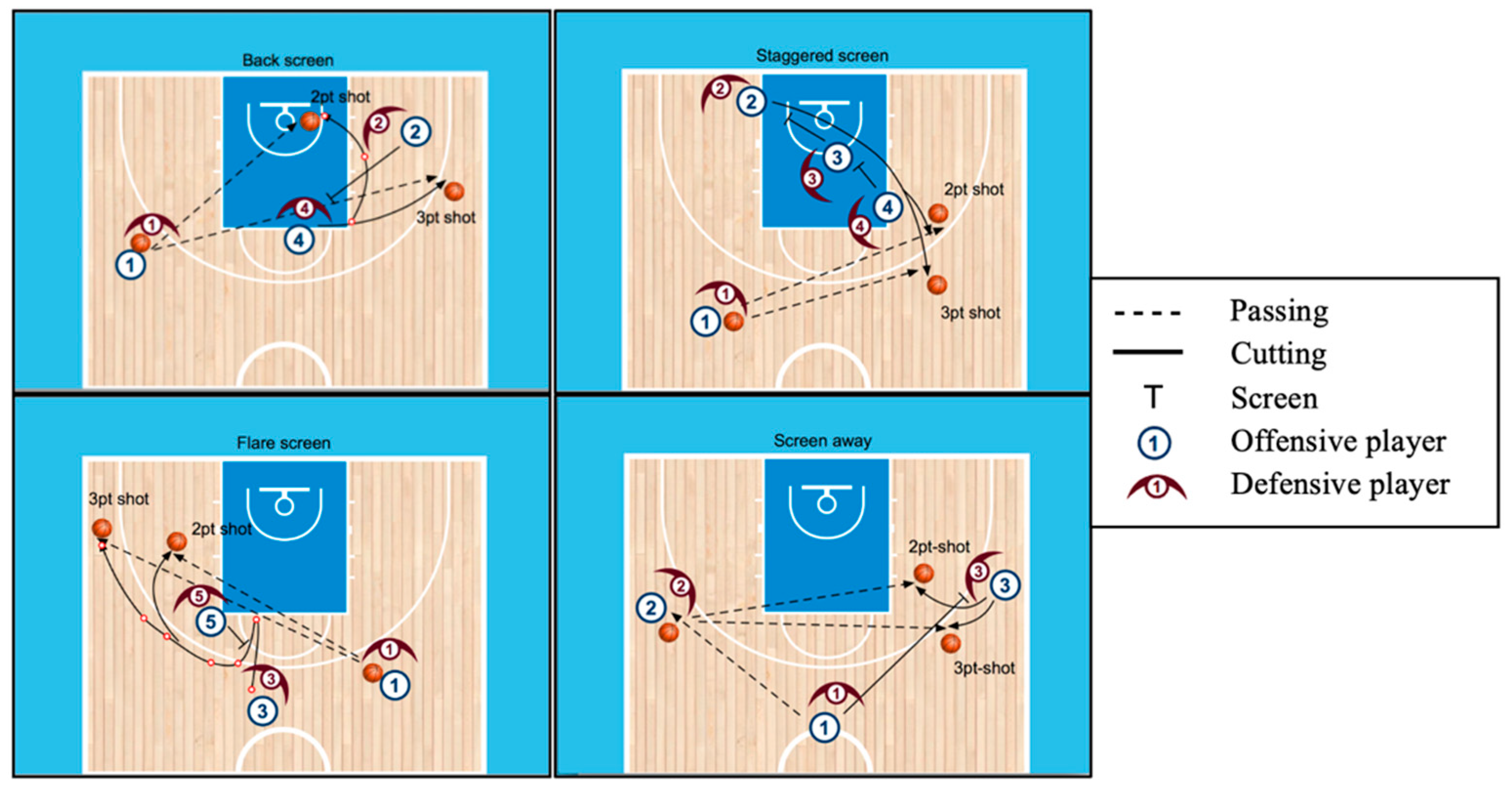
The screen types were defined using standard basketball terminology. More specifically, two consecutive screens for a player, in the same direction away from the ball were defined as a staggered screen. A flare screen was defined as a screen set at the elbow of the free throw line where the player fades out on the weak side. Screen the screener occurs when an offensive player sets a screen and, at the same time, receives a screen from a teammate. To pass on the side and set a screen for a player in the opposite direction was described as a screen away. Down screen is a screen where an offensive player sets himself in a position away from the ball. Back screen occurs when an offensive player stands behind the defensive player with his back toward the basket. Single- and double-staggered screens were combined into one category, as well as the single- and double- high-cross screens. Examples of screen types under consideration are presented in
Figure 1.
We shall note here that not all transitions were observed, for example if the finishing move was a middle-range shot (2-pt), the only possible outcomes would be either a successful or unsuccessful 2-pt shot. For the first-order Markov chain, the possible transitions between states are presented in
Table 3. Apparently, the Markov chain exhibits periodic behavior with period
d = 3, as each screen is always followed by a finishing move and each finishing move is only followed by the outcome of the possession.
It is of interest to examine whether the process
incorporates memory, i.e., a higher-order Markov model would provide a more adequate fit. In relation to basketball, a coach may assume that the outcome of a possession does not only depend on the type of the executed shot, but on the previous characteristics of the phase, such as the type of screen, as it could probably alter the evolution of the possession and provide more space and freedom for a well-executed shot. Hence, we would like to test the null hypothesis that the process is of order r = 1 versus the alternative hypothesis, r = 2. For testing this hypothesis, we used the likelihood ratio test (LRT). The likelihood ratio (LR) is given by
where
and
denote the log-likelihood of models of order 1 and order 2, respectively. The log-likelihood ratio is an essential tool for the comparison of two competing Markov models [
38] and can be used to evaluate well-known goodness-of-fit metrics, such as the AIC and BIC [
39]. The likelihood ratio asymptotically follows a chi-squared distribution with degrees of freedom (df) equal to the difference of degrees of freedom of the two models, thus it can provide a
p-value that can lead to the rejection of the null hypothesis, if it is smaller than a predefined cut-off value α (commonly α is set to 0.05). Adopting the notations of a previous work, where the authors assessed the order of a Markov chain applied in DNA sequences [
40], one can formulate the likelihood ratio for two competing Markov models by
where
denote the number of observed triplets and pairs of
respectively. Also, we note that the ratios
and
are the empirical estimators of the transition probabilities, e.g.,
and
, respectively. The LR could be simplified as
In general, a Markov chain of order r with state space has varying parameters. However, in our case, the number of varying parameters would be less, since in the basketball context the transition probability matrix prohibited some transitions. For example, when the offensive player shoots a 3-pt shot, the possible transitions would not include any other outcome, apart from a successful or missed 3-pt shot. More specifically, the numbers of estimated transition probabilities were 82 and 354 for the first- and second-order Markov chain, respectively. The likelihood ratio value was calculated equal to 395.242, which resulted in , therefore the likelihood ratio test indicated to reject the null hypothesis, in favor of r = 2.
The results of the significant relationships between the three components (screen type, finishing move and outcome) lead to establishing a model that includes second-order dependencies, therefore a second-order Markov chain is proposed to study the effect of screen type and finishing move on the outcome of the possession. The state space
of the second-order Markov chain consists of the ordered pairs of events that belong in the state-space
V of the first-order Markov chain. The transition probabilities are presented in
Table 4, in reduced form. Several considerations were made regarding the time, as a parameter that influences the frequency of specific off-ball screens and outcomes. First, the off-ball screen possessions were designated into two categories, 0–8 s and 8–24 s, according to the shot clock time at the time of the finishing move. For each subsample, the transition probabilities were estimated and the asymptotic probability vectors were also estimated. Second, we differentiated the offensive movements between the first three quarters and the last quarter of the game, where in the last quarter, as the pace of the game increases, the losing team can make a comeback.


