Respondent Burden Effects on Item Non-Response and Careless Response Rates: An Analysis of Two Types of Surveys

Abstract

The respondent burden refers to the effort required by a respondent to answer a questionnaire. Although this concept was introduced decades ago, few studies have focused on the quantitative detection of such a burden. In this paper, a face-to-face survey and a telephone survey conducted in Valencia (Spain) are analyzed. The presence of burden is studied in terms of both item non-response rates and careless response rates. In particular, two moving-window statistics based on the coefficient of unalikeability and the average longstring index are proposed for characterizing careless responding. Item non-response and careless response rates are modeled for each survey by using mixed-effects models, including respondent-level and question-level covariates and also temporal random effects to assess the existence of respondent burden during the questionnaire. The results suggest that the sociodemographic characteristics of the respondents and the typology of the question impact item non-response and careless response rates. Moreover, the estimates of the temporal random effects indicate that item non-response and careless response rates are time-varying, suggesting the presence of respondent burden. In particular, an increasing trend in item non-response rates in the telephone survey has been found, which supports the hypothesis of the burden. Regarding careless responding, despite the presence of some temporal variation, no clear trend has been identified.

1. Introduction

The potential for long and complex surveys to burden respondents has been of concern to researchers for decades. Hence, identifying the existence of some form of respondent burden, determining its potential causes, and mitigating its consequences on survey estimates are essential to ensure that data collected through surveys are reliable and useful for some fields such as the social and health sciences in which surveys are widely used. However, this is a difficult task given the large degree of disagreement that still exists around the drivers and consequences of response burden, as has been revealed in a recent review of the currently available literature [1]. In particular, the authors of this review highlight that response burden is often conceptualized and measured by very different mechanisms.

For instance, in a seminal paper on the topic, Bradburn [2] identified four factors related to the respondent burden: (1) the length of the survey, (2) the effort required to answer, (3) the stress level put on the respondent, and (4) the periodicity with which the respondent is interviewed. Decades later, Haraldsen [3] placed a greater emphasis on respondent characteristics, suggesting that respondent’s competence, interest, and availability are the main factors that favor the appearance of burden.

In addition to the two characterizations of response burden provided by Bradburn and Haraldsen, multiple authors have attempted to measure it in terms of several questionnaire characteristics that presumably impact the appearance of burden. In this regard, Sharp and Frankel [4] conducted the first quantitative research on respondent burden by constructing both objective and subjective indicators of this phenomenon. Objective indicators consisted of measuring concrete behaviors among respondents such as interview breakoffs, lack of answer, or display of restlessness or discomfort. On the other hand, subjective/attitudinal indicators were obtained from a questionnaire that was administered to respondents (once the interview had ended), which asked the participants about their opinion on the length of the interview, the difficulty of the questions, the suitability of the time, the effort required for answering, etc.

Other authors have mainly focused on survey length to control for the presence of response burden. In the context of web surveys, Galesic and Bosnjak [5] showed that the longer the questionnaire, the fewer respondents started and finished it. Moreover, questions positioned later were associated with faster, shorter, and more uniform (less variable) answers than those questions at the beginning of the questionnaire. In the context of health questionnaires, it has been found that longer questionnaires are associated with lower response rates. However, the lack of consideration of the complexity of the questionnaire and the typology of the questions limits the generalizability of the results [6]. Indeed, response burden is likely to be more notorious in a shorter questionnaire including complex questions rather than in a longer questionnaire requiring more simplistic responses. In addition, the sociodemographic characteristics of the respondent may also influence their attitude when responding to the questionnaire [7,8]. In any case, although there seem to be more studies suggesting that a longer questionnaire is associated with lower response rates, some studies have reported mixed results [9]. Indeed, in another meta-analysis, it was concluded that the length of the questionnaire has a minor effect on the response rate [10].

Given the lack of consensus on the causes of the respondent burden, some authors have followed a structural equation modeling approach to determine indicators of response burden [1]. The results pointed out that some specific conditions such as respondent motivation, the existence of respondents with greater difficulties to complete the task (measured as a latent construct accounting for respondent’s age and household structure), and respondents’ perception about the survey have an impact on burden. However, contrary to previous research, these authors did not observe a significant association between response burden and the effort carried out by the participants in terms of certain variables such as the interview length or the number of interviews, among others. Furthermore, these authors found that the mode of data collection, either in person or by telephone, did not have a significant impact on the presence of respondent burden.

The present paper focuses on assessing the potential effects of respondent burden on both item non-response rates and careless response rates. On the one hand, although the study of item non-response rates as a consequence of response burden has already been analyzed by other scholars [11], there is not much literature addressing this issue. Hence, this paper aims to contribute to this topic. Specifically, item non-response rates per question are analyzed based on the position of the question within the questionnaire while also accounting for respondent-level and question-level effects. The objective then is to examine whether item non-response rates follow some temporal pattern that could be attributed to the presence of respondent burden. On the other hand, the relationship between careless responding and respondent burden has also been barely explored, even though some authors have observed a positive association between questionnaire length and careless responding [12,13]. Thus, another objective of the present study is to display how specific statistical metrics can help researchers identify the parts of a questionnaire that might be more strongly associated with careless responding attitudes and which is one possible consequence of the respondent burden. As in the case of item non-response, careless response rates are also modeled to investigate the existence of temporal trends throughout the questionnaire. Finally, the comparison of the differences in these aspects between a questionnaire administered in person and another administered by telephone is also an important part of the study, as multiple studies have shown that the mode of administration of a questionnaire can impact participation levels and the quality of the collected data [14,15,16].

Therefore, the paper is structured as follows. In Section 2, the two survey datasets considered for the research are outlined. Section 3 includes a description of the methods applied for the analysis of item non-response and careless response rates. Section 4 shows the findings achieved for the two surveys under study. Finally, Section 5 provides some concluding remarks.

2. Data

This study used data from two opinion surveys conducted by the City Council of Valencia, the third-largest city of Spain by population. The first survey, referred to as the face-to-face survey, was carried out in December 2019 by personal interviews on the street. A total of 2300 people residing in Valencia were interviewed. The second study, referred to as the telephone survey, was conducted in May 2020 by telephone interviews. In this case, 1150 residents of the city participated. In both surveys, respondents were selected following a quota sampling scheme. In the face-to-face survey, quotas were set on sex, age, nationality, employment situation, and district of residence. A total of 287 sampling locations (obtained randomly and conditional on the spatial distribution of the places of residence of the population of Valencia) were visited by the interviewers to collect the entire sample of respondents. In the telephone survey, quotas were set on sex, age, and household typology. In this case, a telephone directory of residents in Valencia was used to randomly select the respondents. The face-to-face survey contained questions on municipal service and management and specific questions oriented to estimate the level of happiness of the residents of Valencia. By contrast, the telephone survey, which was conducted at the beginning of the COVID-19 pandemic, included several questions on health status, prevention habits, compliance with the rules introduced in response to the COVID-19 crisis, etc.

Both surveys included more than a hundred questions grouped into dozens of sets, referred to as question groups from now on. Hence, if, say, question P.1 is divided into P.1.1, P.1.2, and P.1.3, we are referring to these three items as questions, whereas we refer to P.1 as a question group. Some of the questions were about basic sociodemographic characteristics of the respondents, including age, sex, academic background, employment status, and average household income. Among these, each respondent’s age, sex, and academic background were selected as covariates for the analysis (the other two were discarded because of the presence of a high percentage of missing data). In addition, the following subsection includes a brief description of the types of questions included in both surveys.

Types of Questions

The questions included in the two surveys analyzed were categorized into the following six groups:

• Closed-ended: Questions that force the respondent to choose from a set of alternatives being offered by the interviewer [17]. In the current study, the term "closed-ended question" does not include the Likert scale, rating, and Yes/No questions since these types of questions are treated specifically, as described in the following lines. Therefore, closed-ended questions refer to questions that meet the above definition but do not belong to any of these three more specific types. For instance, the question “What is your current employment situation?” admitting the answers “Employed/Unemployed/Retired/Student/Other” would be considered as a closed-ended question.
• Likert: Questions in which respondents are asked to show their level of agreement (usually, from “strongly disagree” to “strongly agree”) with a given statement [18].
• Multiple answer: Questions that allow the respondent to choose several options from a prespecified set.
• Open-ended: Questions that offer the respondent the possibility of supplying their own answer [17] without being influenced by the interviewer [19].
• Rating: Questions in which respondents have to indicate their level of agreement with a statement through a numerical score within a prespecified range. In contrast to Likert questions, each possible value of a rating scale is not associated with a specific level of agreement/disagreement from a range of answer options.
• Yes/No: Questions in which respondents simply have to say “yes” or “no” (although the answers “don’t know” or “don’t answer” are also allowed).

As can be observed from this grouping of the questions, a distinction has been made between Likert-type and rating-type questions. Although both types of questions yield ordinal responses, rating scales do not necessarily admit a one-to-one identification with a set of answer options (as in the Likert scale). For the two surveys under analysis, most of the rating questions corresponded to 11-point (0–10) scales.

Table 1. Summary of the number of questions and question groups included in each of the surveys studied, in terms of question typology.

	Face-to-Face Survey		Telephone Survey
	Question Groups	Questions	Question Groups	Questions
Closed-ended	9	28	12	27
Likert	4	23	7	24
Multiple answer	1	3	2	5
Open-ended	8	17	9	15
Rating	10	50	4	26
Yes/No	4	19	3	8
Total	36	140	37	105

provides a summary (by question typology) of the number of questions and question groups contained in the two surveys under study. The above-defined types of questions were also used as a covariate for the subsequent analysis of item non-response and careless response rates. As shown in previous studies, question characteristics might have an impact on the respondent burden. For instance, it has been detected that the blocks of questions that include more open-ended questions can be more burdensome when considering an online survey [20].

3. Methodology

The analyses conducted on item non-response and careless response rates for the two survey datasets available are fully described in the following subsections. In particular, the study of careless responding requires the use of specific metrics that are introduced subsequently.

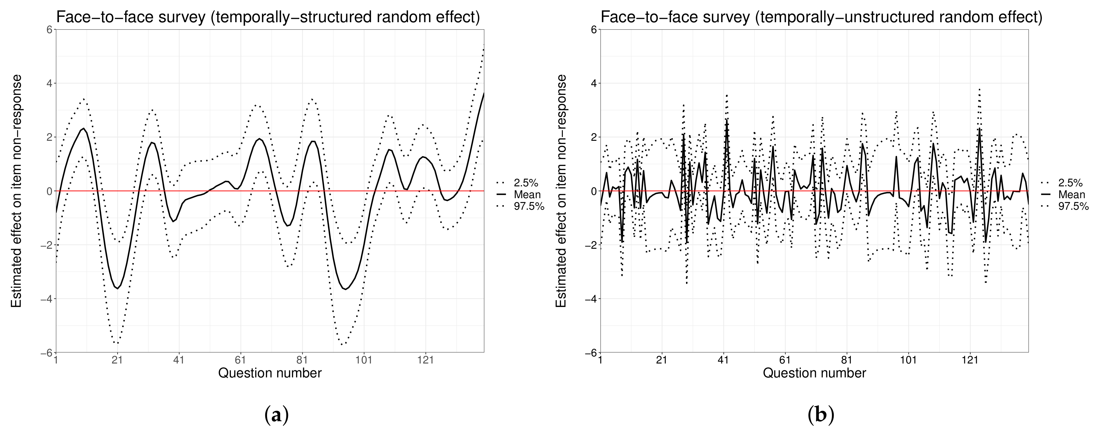
3.1. Modeling Item Non-Response Rates

Item non-response was identified as any response of the form “don’t know” or “don’t answer”. Thus, item non-response was modeled by a Bernoulli random variable, Y∼$B(1,p)$, where p represents the probability that a respondent provides a non-response statement. Specifically, if $Y_{ij}$ is a binary variable that indicates if respondent i provides a non-response statement to question j, the effect of a set of covariates on $Y_{ij}$ can be assessed through a logistic modeling framework [21], which allows establishing the following linear relationship between the logarithm of the odds in favor of the item non-response event (logit transformation) and the covariates:

$$\mathrm{logit}\left(P(Y_{ij}=1)\right)=log\frac{P(Y_{ij}=1)}{P(Y_{ij}=0)}={\beta }_0+\sum _{m=1}^n{\beta }_m{X}_{mi}+{\delta }_j{Q}_j$$

(1)

where ${\beta }_0$ is the intercept term, $X_m$ is a respondent-level covariate, ${\beta }_m$ is a coefficient that measures the effect of covariate $X_m$ on $\mathrm{logit}\left(P(Y_{ij}=1)\right)$, $Q_j$ represents the question typology, and ${\delta }_j$ is a coefficient that measures the effect of the question typology on $\mathrm{logit}\left(P(Y_{ij}=1)\right)$.

In order to assess the presence of respondent burden effects, the model summarized by Equation (1) can be expanded by the inclusion of two temporal random effects, ${\gamma }_j$ and ${\varphi }_j$:

$$\mathrm{logit}\left(P(Y_{ij}=1)\right)=log\frac{P(Y_{ij}=1)}{P(Y_{ij}=0)}={\beta }_0+\sum _{m=1}^n{\beta }_m{X}_{mi}+{\delta }_j{Q}_j+{\gamma }_j+{\varphi }_j$$

(2)

where ${\gamma }_j$ is a temporally-structured random effect, and ${\varphi }_j$ is a temporally-unstructured random effect. The temporally-structured effect, ${\gamma }_j$, was defined in terms of a second-order random walk of the form ${\gamma }_j|{\gamma }_{j-1},{\gamma }_{j-2}$∼$Normal(2{\gamma }_{j-1}+{\gamma }_{j-2},{\sigma }_{\gamma }^2)$, where ${\sigma }_{\gamma }^2$ is the variance component. Regarding the temporally-unstructured effect, an independent and identically distributed Gaussian prior, ${\varphi }_j$∼$Normal(0,{\sigma }_{\varphi }^2)$, was chosen. Thus, the temporal random effects collect some variability at the question level that is not explained by the respondent-level and question-level covariates. Specifically, the temporally-structured random effect captures time trends, whereas the temporally-unstructured random effect captures heterogeneity in the response variable.

Nakagawa’s marginal and conditional $R^2$ coefficients for mixed-effects models are used for measuring the goodness-of-fit of this model [22,23]. The marginal $R^2$, $R_{GLMM\left(m\right)}^2$, represents the proportion of variance explained by fixed effects, whereas the conditional $R^2$, $R_{GLMM\left(c\right)}^2$, indicates the proportion of variance explained by both fixed and random effects.

3.2. Measuring Careless Response

Multiple methods allow measuring the level of careless response presented by an individual answering a questionnaire, each of which offers its advantages and limitations. In particular, certain complications usually arise in the context of complex surveys made of questions of different types, admitting distinct response ranges. For instance, consistency indices such as the even-odd consistency index and the psychometric antonyms index [24] are mostly suitable for questionnaires consisting of numeric items and scales [25]. Other alternatives, such as computing the Mahalanobis distance [26] between the vector containing a person’s responses and the vector containing the “average response” per question in order to detect outliers, rely on the assumption of multivariate normality for the response variable, which rarely holds [25]. The interested reader can find more details about these methods in the literature [24,25,27]. In the present paper, two metrics have been chosen for measuring careless responding: the coefficient of unalikeability and the longstring index.

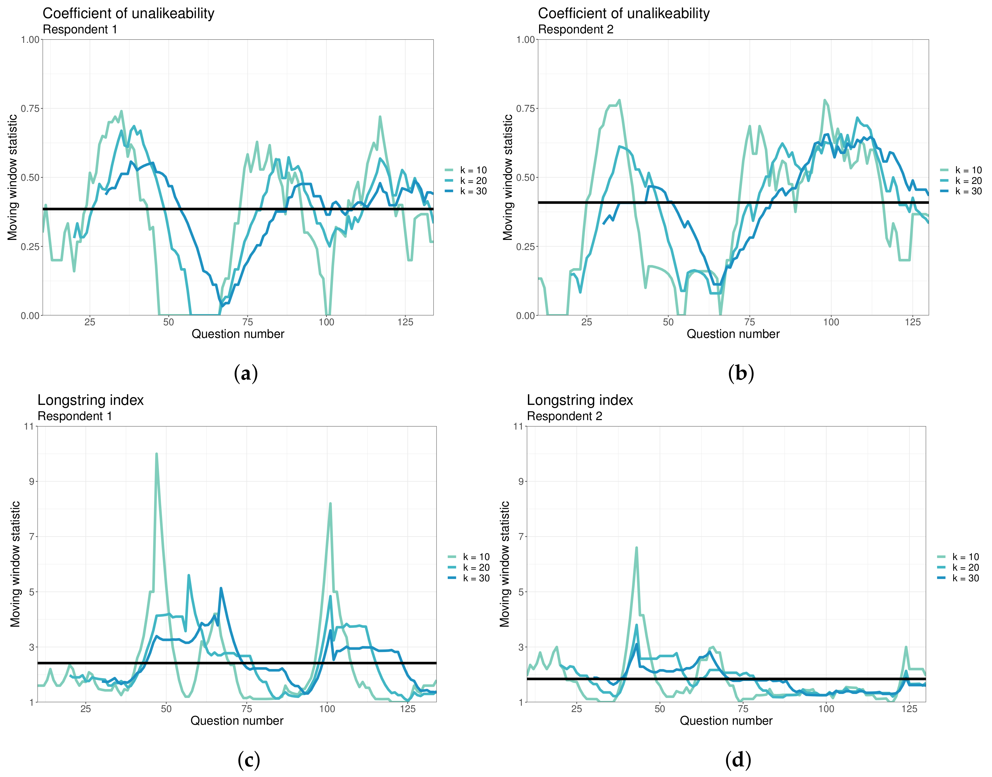
3.2.1. The Coefficient of Unalikeability

The coefficient of unalikeability was introduced by Perry and Kader [28] in order to compute the variability of a finite categorical vector. According to these authors, the unalikeability of a vector can be interpreted as “how often the observations differ from one another” [28]. The coefficient of unalikeability, u, of a categorical vector $\mathit{x}={\left\{x_i\right\}}_{i=1}^n$ is defined as follows:

$$u\left(\mathit{x}\right)=\frac{{\sum }_{i\ne j}c(x_i,x_j)}{n^2-n}$$

where $c(x_i,x_j)=1$ if $x_i\ne x_j$ and 0 otherwise. The coefficient of unalikeability lies in $[0,1]$. A higher value of the coefficient represents greater variation in the data, whereas a lower value means the opposite ($u\left(\mathit{x}\right)=0$ if $\mathit{x}$ is a constant categorical vector). Thus, if $\mathit{x}$ is a vector of responses, a lower value of $u\left(\mathit{x}\right)$ suggests that the respondent is providing identical responses with greater frequency, which is usually associated with careless responding.

The coefficient of unalikeability is conceived for a vector of categorical values that belongs to a unique sample space, that is, a set of possible responses invariant across questions. However, surveys often include multiple types of questions associated with different sample spaces, which prevents one from straightly following the coefficient’s definition. In order to allow the use of the coefficient on the full set of answers relative to a survey provided by an individual, some modifications are required. Hence, the use of the following weighted version of the coefficient according to a survey consisting of G question groups is proposed:

$$\tilde{u}\left(\mathit{x}\right)=\sum _{g=1}^G{w}_{g}u\left({\mathit{x}}_g\right)$$

(3)

where $\mathit{x}=({\mathit{x}}_1,\dots ,{\mathit{x}}_G)$ stands for the responses provided by an individual, ${\mathit{x}}_g$ corresponds to the responses to group $g\in \{1,\dots ,G\}$, and $w_g=\frac{|{\mathit{x}}_g|}{\left|\mathit{x}\right|}$ is the weight that question group $g\in \{1,\dots ,G\}$ represents within the survey ($|·|$ denotes the length of a vector of responses).

3.2.2. The Longstring Index

The maximum longstring, defined as the maximum number of times a respondent chooses the same response option consecutively, is another common method for detecting careless responding. Alternatively, one can also compute the average longstring index of a categorical vector, which is the average length of consecutive identical responses [25,29]. For instance, considering the categorical vector $\mathit{x}=(1,1,1,1,2,2,2,3,3)$, its maximum longstring is 4 (which corresponds to the length of the longest consecutive string of identical responses, formed by four 1 s). By contrast, its average longstring index is 3 (the average between 4, 3, and 2; the lengths of the three consecutive strings of identical responses included in $\mathit{x}$). In the present research, the average longstring index is chosen for analyzing the survey data considered. Thus, given a categorical vector $\mathit{x}$, $\ell \left(\mathit{x}\right)$ is used to denote the average longstring index of $\mathit{x}$. As in the case of the coefficient of unalikeability, the longstring index is weighted according to the structure of the survey following Equation (3), which yields a weighted value $\tilde{\ell }\left(\mathit{x}\right)$, given a vector of responses $\mathit{x}$.

A higher value of the average longstring index indicates that the respondent shows a greater tendency towards consecutive identical responses. Although this might sometimes result from attentive and consistent answers, a high average longstring index is usually associated with careless responding. It is expected that the values of the coefficient of unalikeability and the longstring index corresponding to a set of responses show, to some extent, an opposite behavior. Indeed, higher values of the coefficient of unalikeability should generally yield a lower longstring index and vice versa.

3.2.3. Moving-Window Metrics

Given the complete set of responses that an individual provides to a survey, denoted by $\mathit{x}$, the use of either $\tilde{u}\left(\mathit{x}\right)$ or $\tilde{\ell }\left(\mathit{x}\right)$ allows us to know the overall level of careless response provided by that individual but not how his/her level of attention varied throughout the survey. Hence, in order to capture how an individual’s attentiveness may change over time, a moving-window metric associated with either the coefficient of unalikeability or the longstring average index is constructed. These two moving-window metrics are denoted by ${\tilde{u}}_{mov}\left(\mathit{x}\right)$ and ${\tilde{\ell }}_{mov}\left(\mathit{x}\right)$, and they are computed as follows (only the case of ${\tilde{u}}_{mov}$ is shown as both are analogous):

$${\left({\tilde{u}}_{mov}\right)}_j=\tilde{u}(x_{j-k+1},\dots ,x_j), j\ge k$$

where k represents the period of the moving-window metric. Thus, the jth element of the moving-window metric is computed by applying either $\tilde{u}$ or $\tilde{\ell }$ to the set of k responses spanning from response $j-k+1$ to response j. The choice of a small k provides an accurate picture of the level of attention offered by the respondent, based on the two metrics considered, but it also can result in noisy time series. Conversely, choosing a value of k that is too large could render it impossible to observe any trend. For this reason, an intermediate value of k should be chosen, depending on the number of questions available in the survey. The main functions that were built in R to study careless responding attitudes among respondents are provided in Appendix A.

As an illustration, Figure 1 shows the moving-window metrics corresponding to two of the respondents of the face-to-face survey considering $k\in \{10,20,30\}$. A value of $k=20$ was finally chosen to conduct the analysis in this case.

Table 2. Summary statistics of the two moving-window metrics defined in Section 3.2 (considering $k=20$) for the face-to-face and telephone surveys under analysis.

	Face-to-Face Survey		Telephone Survey
	${\tilde{\mathit{u}}}_{\mathit{mov}}$	${\tilde{\ell }}_{\mathit{mov}}$	${\tilde{\mathit{u}}}_{\mathit{mov}}$	${\tilde{\ell }}_{\mathit{mov}}$
Min.	0.00	1.00	0.00	1.00
1st Qu.	0.30	1.36	0.30	1.22
Median	0.43	1.61	0.42	1.40
Mean	0.42	1.89	0.42	1.63
3rd Qu.	0.53	2.06	0.54	1.77
Max.	0.81	11.60	0.82	7.20

provides a summary of the values corresponding to the moving-window metrics for the two surveys under study.

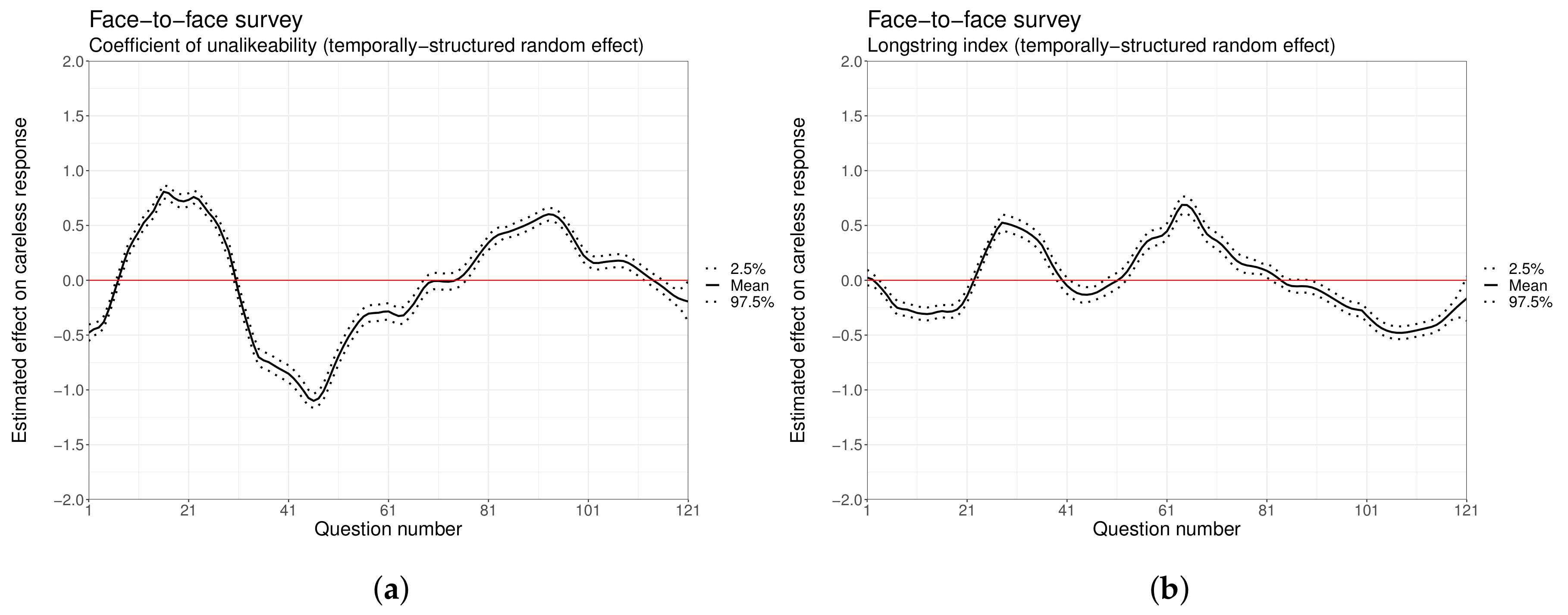
3.3. Modeling Careless Response

Having estimated careless response levels with either the coefficient of unalikeability or the longstring index, modeling these values in terms of the respondent-level and question-level covariates allows assessing which factors may increase careless response rates and how the intensity of careless responding may evolve over time. As with the item non-response rates, a mixed-effects model is considered for each of the metrics. The longstring index is assumed to be normally distributed, so a classical linear mixed-effects model is used [30]. By contrast, since the coefficient of unalikeability lies in $[0,1]$, this metric is modeled through a Beta distribution [31] after applying a widely used transformation to avoid the presence of 0 and 1 values [32]. Specifically, if ${\left({\tilde{u}}_{mov}\right)}_{ij}$∼$\mathrm{Beta}(a_{ij},b_{ij})$, then ${\mu }_{ij}=\frac{a_{ij}}{a_{ij}+b_{ij}}$ represents the mean value of this distribution and, therefore, the logit of ${\mu }_{ij}$ can be modeled in terms of a linear predictor (as in the logistic model). Thus, the following two separate mixed-effects models were considered for modeling the mean value of ${\left({\tilde{u}}_{mov}\right)}_{ij}$ and ${({\tilde{\ell }}_{mov})}_{ij}$, respectively:

$$\mathrm{logit}\left({\mu }_{ij}\right)=log\frac{{\mu }_{ij}}{1-{\mu }_{ij}}={\beta }_0+\sum _{m=1}^n{\beta }_m{X}_{mi}+{\delta }_j{Q}_j^k+{\gamma }_j+{\varphi }_j$$

(4)

$${({\tilde{\ell }}_{mov})}_{ij}={\beta }_0+\sum _{m=1}^n{\beta }_m{X}_{mi}+{\delta }_j{Q}_j^k+{\gamma }_j+{\varphi }_j$$

(5)

where parameters ${\beta }_0$, ${\beta }_m$, ${\delta }_j$, ${\gamma }_j$, and ${\varphi }_j$ roughly have the same meaning/interpretation than in Equation (2). In this case, however, due to definition of the moving-window metrics, the inclusion of question typology in the model needs to be reconsidered. Thus, $Q_j^k$ represents the most frequent question typology among questions $j-k+1$ to j of the questionnaire. A “Tie” category is created to account for the cases of multiple types of questions with the same frequency. As with the case of the mixed-effects logistic model, Nakagawa’s marginal and conditional $R^2$ coefficients are employed for assessing the goodness-of-fit of these models.

3.4. Software

All the analyses were carried out in the 4.0 version of the R programming language [33]. In particular, the R packages careless [29], ggplot2 [34], INLA [35,36], and ragree [37] were required for some specific parts of the study.

4. Results

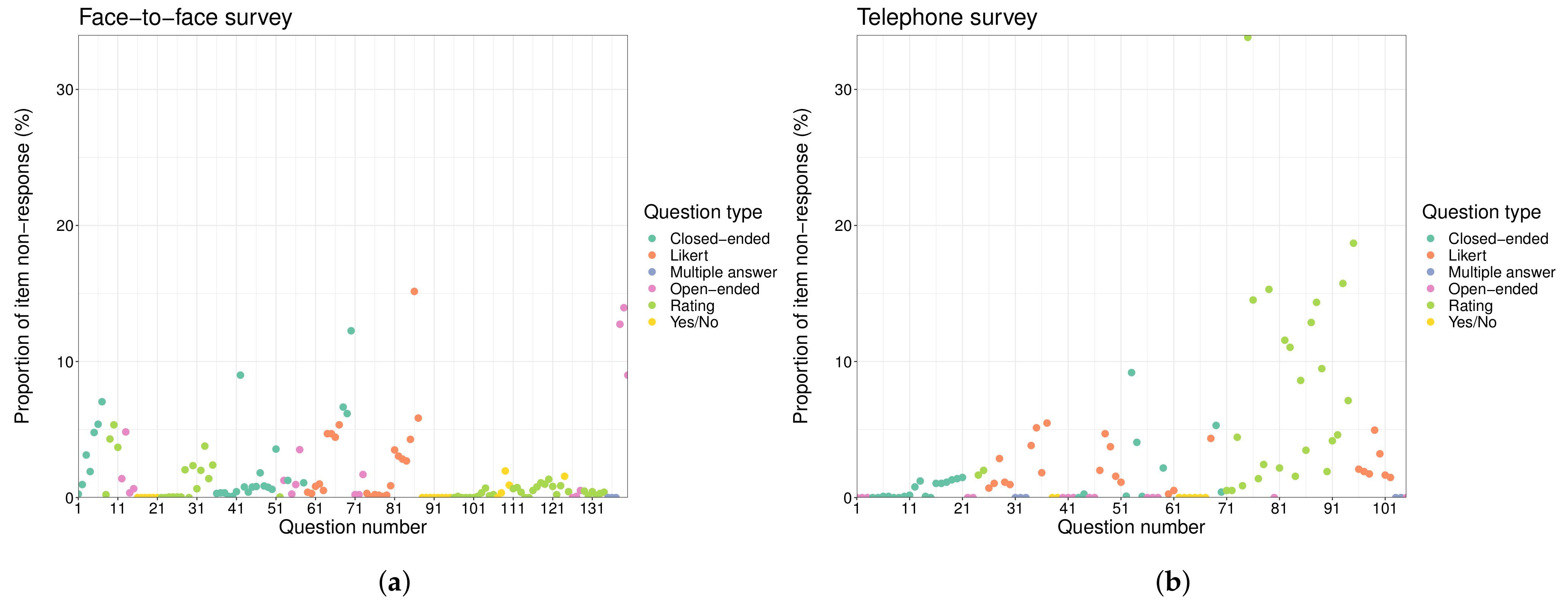
4.1. Item Non-Response

Figure 2 shows the proportion of item non-response found in each of the questions of the two surveys considered for the analysis.

Table 3. Fixed-effect estimates corresponding to the modeling of the item non-response values, following Equation (2), in terms of the mean of the posterior distribution of each parameter involved. The lower (Low) and upper (Up) bounds of the 95% credibility interval associated with each estimate are also provided.

		Face-to-Face Survey			Telephone Survey
		Mean	Low	Up	Mean	Low	Up
Intercept		−3.09	−4.31	−1.86	−2.86	−3.47	−2.27
Age	<40
	40–64	0.04	−0.04	0.12	−0.49	−0.59	−0.38
	≥65	0.12	0.03	0.21	0.17	0.05	0.28
Sex	Male
	Female	0.07	0.00	0.13	0.45	0.37	0.53
Academic level	No studies
	Secondary	−0.15	−0.30	0.00	−0.51	−0.65	−0.36
	High-school	−0.19	−0.33	−0.04	−1.12	−1.27	−0.96
	University	−0.48	−0.64	−0.32	−1.33	−1.49	−1.16
Question typology	Likert
	Closed-ended	0.48	−1.04	1.99	−0.46	−1.43	0.51
	Multiple answer	−11.24	−33.61	2.49	−10.03	−33.26	4.16
	Open-ended	−0.37	−1.89	1.13	−10.21	−33.14	3.87
	Rating	−1.00	−2.66	0.64	0.77	−0.16	1.68
	Yes/No	−2.25	−4.06	−0.51	−9.60	−33.24	4.86
$R_{GLMM\left(m\right)}^2$		0.2848			0.7339
$R_{GLMM\left(c\right)}^2$		0.6847			0.8455

contains the fixed-effects estimates obtained after fitting the logistic model indicated in Equation (2). For each of the (categorical) covariates considered at the individual or the question level, a reference level is used to which all of the other levels are compared (the reference level is the one for which the corresponding row is left blank in Table 3) so that each estimate must be interpreted with regard to the corresponding reference level. As the covariates have not been standardized, the fixed-effects estimates corresponding to different covariates are not comparable (the focus is only placed on the statistical significance and sign of each estimate). The $R_{GLMM\left(m\right)}^2$ and $R_{GLMM\left(c\right)}^2$ values are also provided in Table 3.

Thus, several parameter estimates are statistically significant and consistent in terms of their sign across the two surveys considered. In particular, older respondents (those aged 65 years and over) and females present higher item non-response rates, whereas having a higher academic level is associated with lower item non-response rates. Moreover, it is worth noting that respondents aged 40–64 present lower item non-response rates than those aged less than 40 only in the telephone survey. Regarding question typology, there is a greater level of inconsistency across the surveys, and only the parameter estimate corresponding to Yes/No questions is statistically significant in the case of the face-to-face survey.

The estimates corresponding to the two temporal random effects included in the model are shown in Figure 3 (for the face-to-face survey) and Figure 4 (for the telephone survey). Specifically, Figure 3a and Figure 4b display the estimation of the structured temporal effect (based on a second-order random walk), while Figure 3b and Figure 4b show the estimation of the unstructured temporal effect, which accounts for uncorrelated heterogeneity in item non-response rates. In light of the estimates obtained for the structured random effects, it can be concluded that the temporal evolution of item non-response rates varied significantly from one survey to another. In the face-to-face survey, no clear trend is observed as the question-level estimate of the structured random effect exhibits multiple variations in terms of sign. For instance, the temporally-structured random effect is positive for the first questions, then becomes negative, and turns positive again at the 30th question. This changing behavior of item non-response rates remains for the rest of the questionnaire. On the contrary, the telephone survey presents a very clear trend regarding the evolution of item non-response rates, which progressively grow over time. This increasing trend in item non-response rates, while accounting for several individual-level and question-level covariates, suggests the presence of respondent burden. In fact, the temporal random effects help to explain the variability in item non-response rates, as suggested by the improvement of the $R_{GLMM\left(c\right)}^2$ over the $R_{GLMM\left(m\right)}^2$ values (Table 3).

4.2. Careless Response

Table 4. Fixed-effect estimates corresponding to the modeling of the coefficient of unalikeability, following Equation (4), in terms of the mean of the posterior distribution of each parameter involved. The lower (Low) and upper (Up) bounds of the 95% credibility interval associated with each estimate are also provided.

		Face-to-Face Survey			Telephone Survey
		Mean	Low	Up	Mean	Low	Up
Intercept		−0.46	−0.53	−0.39	−0.37	−0.46	−0.28
Age	<40
	40–64	0.01	0.00	0.01	−0.07	−0.07	−0.06
	≥65	0.05	0.04	0.06	−0.03	−0.04	−0.01
Sex	Male
	Female	0.01	0.01	0.01	−0.04	−0.05	−0.03
Academic level	No studies
	Secondary	0.03	0.02	0.04	−0.14	−0.16	−0.12
	High-school	0.02	0.01	0.03	0.01	−0.01	0.03
	University	0.08	0.07	0.10	0.03	0.01	0.05
Most frequent question typology	Likert
	Closed-ended	−0.01	−0.09	0.08	−0.07	−0.19	0.05
	Open-ended	-	-	-	0.17	−0.00	0.36
	Rating	0.02	−0.09	0.12	−0.00	−0.20	0.20
	Tie	0.01	−0.08	0.09	−0.02	−0.12	0.09
	Yes/No	−0.01	−0.11	0.09	−0.03	−0.18	0.12
$R_{GLMM\left(m\right)}^2$		0.0040			0.0206
$R_{GLMM\left(c\right)}^2$		0.1263			0.1490

and

Table 5. Fixed-effect estimates corresponding to the modeling of the longstring index, following Equation (5), in terms of the mean of the posterior distribution of each parameter involved. The lower (Low) and upper (Up) bounds of the 95% credibility interval associated with each estimate are also provided.

		Face-to-Face Survey			Telephone Survey
		Mean	Low	Up	Mean	Low	Up
Intercept		1.97	1.90	2.04	1.61	1.57	1.66
Age	<40
	40-64	−0.02	−0.03	−0.02	0.05	0.04	0.06
	≥65	−0.09	−0.10	−0.08	0.07	0.06	0.09
Sex	Male
	Female	−0.01	−0.02	−0.01	0.05	0.04	0.06
Academic level	No studies
	Secondary	−0.05	−0.06	−0.03	0.06	0.04	0.09
	High-school	−0.03	−0.05	−0.01	−0.09	−0.11	−0.06
	University	−0.12	−0.13	−0.10	−0.13	−0.16	−0.11
Most frequent question typology	Likert
	Closed-ended	−0.03	−0.11	0.05	−0.06	−0.11	−0.01
	Open-ended	−	−	−	−0.00	−0.08	0.07
	Rating	0.04	−0.07	0.15	−0.04	−0.12	0.05
	Tie	0.00	−0.08	0.08	−0.03	−0.07	0.02
	Yes/No	−0.03	−0.12	0.07	−0.02	−0.09	0.04
$R_{GLMM\left(m\right)}^2$		0.0031			0.0132
$R_{GLMM\left(c\right)}^2$		0.6538			0.7532

show the fixed-effects estimates corresponding to the mixed-effects models represented by Equations (4) and (5). As in Table 3, the estimates provided in Table 4 and Table 5 must be interpreted with respect to the corresponding reference level, and they are also not comparable across different covariates. It should be noted that the sign of the estimates of Table 4 and Table 5 have the opposite meaning depending on the metric being considered. Indeed, whereas in Table 4 a (statistically significant) negative estimate indicates that the corresponding categorical level increases careless responding rates, in Table 5 a (statistically significant) negative estimate represents the opposite tendency. The $R_{GLMM\left(m\right)}^2$ and $R_{GLMM\left(c\right)}^2$ values are also displayed in Table 4 and Table 5.

Regarding the analysis of the coefficient of unalikeability (Table 4), the results suggest that respondents aged less than 40 years showed a greater tendency towards careless responding than those aged 40 years and over in the case of the face-to-face survey. By contrast, the same age group presents the opposite behavior in the context of the telephone survey. There is also disagreement on the effect of the sex of the respondent on careless response rates, as females showed a greater tendency towards careless responding than males in the context of the telephone survey, but the opposite tendency in the face-to-face survey is observed. Concerning academic levels, in general, respondents with some academic background exhibited more attentive behavior than respondents with no studies (except for the respondents with secondary education in the case of the telephone survey). Finally, the abundance of open-ended questions seems to be associated with a lower tendency towards careless responses in the telephone survey analyzed (compared to Likert questions).

On the other hand, the results obtained by modeling the longstring index values are highly coherent with those of the coefficient of unalikeability (Table 5). The most remarkable difference is that the analysis of the longstring values reveals that the abundance of closed-ended questions is associated with an increase in careless response rates in the telephone survey (compared to Likert questions). By contrast, the effects of the respondent’s age, sex, and academic level have remained consistent with those found by using the analysis of the coefficient of unalikeability.

Furthermore, in order to evaluate if the incidence of careless responding might be affected by a respondent burden effect, the estimates corresponding to the temporal random effects defined in Equations (4) and (5) are analyzed. Figure 5a and Figure 6a display the estimation of the structured temporal effect implicated in the modeling of the coefficient of unalikeability, whereas Figure 5b and Figure 6b show the analogous estimation that corresponds to the modeling of longstring index values. The interpretation of the temporal random effects in the case of the careless response rates is more challenging than in the item non-response rates, and the two moving-window metrics defined partially disagree with one another. In particular, the temporal effects estimated on the telephone survey (Figure 6) are quite similar for both metrics: the estimates are positive at the beginning of the questionnaire until, approximately, question number 20, they start to decrease and become negative at the central part of the questionnaire and grow again towards positive values from approximately question number 50. However, given that observing higher values for the coefficient of unalikeability means the opposite compared to observing higher values for the longstring index, it is very hard to conclude about respondent burden effects on careless responding. Nevertheless, it may be worth noting that the longstring index showed a tendency towards higher values at the beginning of the telephone survey, whereas the coefficient of unalikeability displayed a similar behavior at the end of the telephone survey. In the case of the face-to-face survey, no clear trend is appreciated for any of the metrics (Figure 5). However, the variability of the estimated temporally-structured effects is remarkable (Figure 5b), displaying multiple peaks and valleys throughout the questionnaire. Hence, although there is no evident relationship between question number and careless response rates, it seems clear that careless response rates evolved since the administration of the questionnaire started. Indeed, the $R_{GLMM\left(c\right)}^2$ values, which account for the contribution of random effects to model fitting, are considerably higher than the $R_{GLMM\left(m\right)}^2$ values (Table 4 and Table 5).

5. Discussion and Conclusions

There are two main types of methodologies available for measuring respondent burden: those that explicitly measure the level of burden experienced by the respondent throughout the interview and those that indirectly assess the existence of respondent burden by the subsequent analysis of respondents’ answers. In this paper, the latter of these two methodologies has been followed in order to evaluate the existence of a temporal structure in either item non-response or careless response rates that might reflect the presence of respondent burden. In particular, a model-based analysis of both item non-response and careless response rates (as two likely consequences of respondent burden) is proposed, which allows accounting for respondent-level and question-level covariates too. Hence, the analysis has reflected some knowledge on how certain sociodemographic and question-level covariates might impact these rates. Moreover, the incorporation of temporal random effects in the models has enabled accounting for respondent burden effects, meaning the impact of question number on item non-response and careless response rates. Anyhow, it is worth noting that this might be an oversimplification of respondent burden effects, and indeed there is still great uncertainty about how such burden influences the respondent. First, it has been shown that subjective perceptions of burden may not be strongly correlated with the true level of burden faced [38]. Moreover, as another important limitation, Bradburn already pointed out the difficulty of establishing a relationship between the level of burden that a respondent can potentially accept and the importance of the data being collected by the survey [2]. In the case of the two surveys analyzed in this study, we can assume that the one conducted by telephone during the early phase of the COVID-19 crisis (to build up knowledge regarding citizen response against the pandemic) must have aroused great interest among respondents. Despite this fact, the effects of the respondent burden were apparently stronger in terms of item non-response rates in the telephone survey rather than in the face-to-face survey, even though the latter did not focus on a hot topic. In order to avoid the circumstance where the topic of the questionnaire affects the results, it would be advisable to conduct a single questionnaire in the different modes of administration available. Furthermore, it should be noted that even though some evidence has been found on the potential prevalence of response burden as a consequence of questionnaire length, the implementation of very short questionnaires is not always advisable, as has been shown in the context of some fields such as psychometrics [39,40].

In addition to the difficulty of delimiting respondent burden effects and separating them from the context in which the survey is conducted, the quantification of careless responding is a highly complex task. It can be approached by using multiple alternative metrics, including the coefficient of unalikeability and the longstring index, which were the two finally chosen for performing this study. These two metrics have at least four advantageous properties: easily interpretable, computationally inexpensive, adaptable to multiple types of questions, and definable as moving-window metrics. The latter property is essential for allowing the study of respondent burden. Hence, the use of the moving-window statistics proposed in this paper, or other alternatives of similar nature, could be helpful for detecting (at the pretest stage) the parts of a questionnaire that are more prone to yield careless responses in order to be able to adjust it accordingly. However, it is also necessary to mention that these metrics are limited, and their interpretation may not always be straightforward. Specifically, in this study, it has been assumed that a low value of the unalikeability coefficient, which implies little variability in the responses, is associated with a careless responding attitude (similar to what is provided by the longstring index). However, some authors have shown that the high variability in a set of responses (considering a five item Likert scale) indicates the existence of randomness in the response [41]. Therefore, these types of metrics should be used with caution and may preferably be used as an exploratory tool and accompanied by a qualitative analysis of the questionnaire.

References

1. Yan, T.; Fricker, S.; Tsai, S. Response Burden: What Is It and What Predicts It? In Advances in Questionnaire Design, Development, Evaluation and Testing; John Wiley & Sons: Hoboken, NJ, USA, 2020; pp. 193–212. [Google Scholar]
2. Bradburn, N. Respondent burden. In Proceedings of the Survey Research Methods Section of the American Statistical Association; American Statistical Association: Alexandria, VA, USA, 1978; Volume 35, pp. 35–40. [Google Scholar]
3. Haraldsen, G. Identifying and Reducing Response Burdens in Internet Business Surveys. J. Off. Stat. 2004, 20, 393–410. [Google Scholar]
4. Sharp, L.M.; Frankel, J. Respondent burden: A test of some common assumptions. Public Opin. Q. 1983, 47, 36–53. [Google Scholar] [CrossRef]
5. Galesic, M.; Bosnjak, M. Effects of questionnaire length on participation and indicators of response quality in a web survey. Public Opin. Q. 2009, 73, 349–360. [Google Scholar] [CrossRef]
6. Rolstad, S.; Adler, J.; Rydén, A. Response burden and questionnaire length: Is shorter better? A review and meta-analysis. Value Health 2011, 14, 1101–1108. [Google Scholar] [CrossRef] [PubMed] [Green Version]
7. Olson, K.; Smyth, J.D.; Ganshert, A. The effects of respondent and question characteristics on respondent answering behaviors in telephone interviews. J. Surv. Stat. Methodol. 2019, 7, 275–308. [Google Scholar] [CrossRef] [Green Version]
8. Sun, H.; Conrad, F.G.; Kreuter, F. The Relationship between Interviewer-Respondent Rapport and Data Quality. J. Surv. Stat. Methodol. 2021, 9, 429–448. [Google Scholar] [CrossRef]
9. Bogen, K. The effect of questionnaire length on response rates: A review of the literature. In Survey Research Methods Section of the American Statistical Association; U.S. Census Bureau: Suitland, MD, USA, 1996; pp. 1020–1025. [Google Scholar]
10. Cook, C.; Heath, F.; Thompson, R.L. A meta-analysis of response rates in web-or internet-based surveys. Educ. Psychol. Meas. 2000, 60, 821–836. [Google Scholar] [CrossRef]
11. Warriner, G.K. Accuracy of self-reports to the burdensome question: Survey response and nonresponse error trade-offs. Qual. Quant. 1991, 25, 253–269. [Google Scholar] [CrossRef]
12. Brower, C.K. Too Long and too Boring: The Effects of Survey Length and Interest on Careless Responding. Master’s Thesis, Wright State University, Dayton, OH, USA, 2018. [Google Scholar]
13. Gibson, A.M.; Bowling, N.A. The effects of questionnaire length and behavioral consequences on careless responding. Eur. J. Psychol. Assess. 2020, 36, 410–420. [Google Scholar] [CrossRef]
14. Denscombe, M. Item non-response rates: A comparison of online and paper questionnaires. Int. J. Soc. Res. Methodol. 2009, 12, 281–291. [Google Scholar] [CrossRef]
15. Scott, A.; Jeon, S.H.; Joyce, C.M.; Humphreys, J.S.; Kalb, G.; Witt, J.; Leahy, A. A randomised trial and economic evaluation of the effect of response mode on response rate, response bias, and item non-response in a survey of doctors. BMC Med. Res. Methodol. 2011, 11, 126. [Google Scholar] [CrossRef] [Green Version]
16. Dupuis, M.; Strippoli, M.P.F.; Gholam-Rezaee, M.; Preisig, M.; Vandeleur, C.L. Mental disorders, attrition at follow-up, and questionnaire non-completion in epidemiologic research. Illustrations from the CoLaus| PsyCoLaus study. Int. J. Methods Psychiatr. Res. 2019, 28, e1805. [Google Scholar] [CrossRef] [PubMed]
17. Foddy, W. Constructing Questions for Interviews and Questionnaires: Theory and Practice in Social Research; Cambridge University Press: Cambridge, UK, 1994. [Google Scholar]
18. Joshi, A.; Kale, S.; Chandel, S.; Pal, D.K. Likert scale: Explored and explained. Curr. J. Appl. Sci. Technol. 2015, 7, 396–403. [Google Scholar] [CrossRef]
19. Reja, U.; Manfreda, K.L.; Hlebec, V.; Vehovar, V. Open-ended vs. close-ended questions in web questionnaires. Dev. Appl. Stat. 2003, 19, 159–177. [Google Scholar]
20. Galesic, M. Dropouts on the web: Effects of interest and burden experienced during an online survey. J. Off. Stat. 2006, 22, 313. [Google Scholar]
21. Agresti, A. An Introduction to Categorical Data Analysis; John Wiley & Sons: Hoboken, NJ, USA, 2018. [Google Scholar]
22. Nakagawa, S.; Schielzeth, H. A general and simple method for obtaining R2 from generalized linear mixed-effects models. Methods Ecol. Evol. 2013, 4, 133–142. [Google Scholar] [CrossRef]
23. Nakagawa, S.; Johnson, P.C.; Schielzeth, H. The coefficient of determination R2 and intra-class correlation coefficient from generalized linear mixed-effects models revisited and expanded. J. R. Soc. Interface 2017, 14, 20170213. [Google Scholar] [CrossRef] [PubMed] [Green Version]
24. Meade, A.W.; Craig, S.B. Identifying careless responses in survey data. Psychol. Methods 2012, 17, 437. [Google Scholar] [CrossRef] [PubMed] [Green Version]
25. Niessen, A.S.M.; Meijer, R.R.; Tendeiro, J.N. Detecting careless respondents in web-based questionnaires: Which method to use? J. Res. Personal. 2016, 63, 1–11. [Google Scholar] [CrossRef] [Green Version]
26. Mahalanobis, P.C. On the generalized distance in statistics. Proc. Natl. Inst. Sci. India 1936, 2, 49–55. [Google Scholar]
27. Dupuis, M.; Meier, E.; Cuneo, F. Detecting computer-generated random responding in questionnaire-based data: A comparison of seven indices. Behav. Res. Methods 2019, 51, 2228–2237. [Google Scholar] [CrossRef] [PubMed]
28. Perry, M.; Kader, G. Variation as unalikeability. Teach. Stat. 2005, 27, 58–60. [Google Scholar] [CrossRef]
29. Yentes, R.D.; Wilhelm, F. Careless: Procedures for Computing Indices of Careless Responding, R Package Version 1.1.3; 2018. Available online: http://r.meteo.uni.wroc.pl/web/packages/careless/index.html (accessed on 18 August 2021).
30. Oberg, A.L.; Mahoney, D.W. Linear Mixed Effects Models. In Topics in Biostatistics; Humana Press: Totowa, NJ, USA, 2007; pp. 213–234. [Google Scholar]
31. Ferrari, S.; Cribari-Neto, F. Beta regression for modelling rates and proportions. J. Appl. Stat. 2004, 31, 799–815. [Google Scholar] [CrossRef]
32. Smithson, M.; Verkuilen, J. A better lemon squeezer? Maximum-likelihood regression with beta-distributed dependent variables. Psychol. Methods 2006, 11, 54. [Google Scholar] [CrossRef] [PubMed] [Green Version]
33. R Core Team. R Language Definition; R Foundation for Statistical Computing: Vienna, Austria, 2020. [Google Scholar]
34. Wickham, H. ggplot2: Elegant Graphics for Data Analysis; Springer: New York, NY, USA, 2016. [Google Scholar]
35. Rue, H.; Martino, S.; Chopin, N. Approximate Bayesian Inference for Latent Gaussian Models Using Integrated Nested Laplace Approximations (with discussion). J. R. Stat. Soc. B 2009, 71, 319–392. [Google Scholar] [CrossRef]
36. Lindgren, F.; Rue, H. Bayesian Spatial Modelling with R-INLA. J. Stat. Softw. 2015, 63, 1–25. [Google Scholar] [CrossRef] [Green Version]
37. Redd, R. Ragree: Rater Agreement, R Package Version 0.0.4; 2020. Available online: https://rdrr.io/github/raredd/ragree/ (accessed on 18 August 2021).
38. Read, B. Respondent burden in a Mobile App: Evidence from a shopping receipt scanning study. Surv. Res. Methods 2019, 13, 45–71. [Google Scholar]
39. Schweizer, K. Some Thoughts Concerning the Recent Shift from Measures with Many Items to Measures with Few Items. Eur. J. Psychol. Assess. 2011, 27, 71–72. [Google Scholar] [CrossRef]
40. Rammstedt, B.; Beierlein, C. Can’t we make it any shorter? The limits of personality assessment and ways to overcome them. J. Individ. Differ. 2014, 35, 212–220. [Google Scholar] [CrossRef]
41. Marjanovic, Z.; Holden, R.; Struthers, W.; Cribbie, R.; Greenglass, E. The inter-item standard deviation (ISD): An index that discriminates between conscientious and random responders. Personal. Individ. Differ. 2015, 84, 79–83. [Google Scholar] [CrossRef] [Green Version]
Figure 1. Example of application of the two moving-window metrics defined in Section 3.2, considering two different respondents to the face-to-face survey studied and k { 10 , 20 , 30 } . Specifically, the values of u ˜ m o v ( x ) for respondents 1 and 2 are shown in (a,b), respectively, whereas the corresponding values of ˜ m o v ( x ) are shown in (c,d). The black horizontal line represents the average value of the moving-window metric for the respondent.
Mathematics 09 02035 g001
Figure 2. Proportion of item non-response observed for each of the questions included in the face-to-face (a) and the telephone survey (b) studied. The points are coloured according to question typology.
Mathematics 09 02035 g002
Figure 3. Estimation of the structured (a) and unstructured (b) temporal random effects considered for modeling item non-response values in the face-to-face survey. These estimates correspond to γ ^ j (a) and ϕ ^ j (b) according to Equation (2).
Mathematics 09 02035 g003
Figure 4. Estimation of the structured (a) and unstructured (b) temporal random effects considered for modeling item non-response values in the telephone survey. These estimates correspond to γ ^ j (a) and ϕ ^ j (b) according to Equation (2).
Mathematics 09 02035 g004
Figure 5. Estimation of the structured temporal random effect included for modeling careless response rates in the face-to-face survey by considering the coefficient of unalikeability (a) and the longstring index (b). These estimates correspond to γ ^ j according to Equation (4) (a) and Equation 5 (b).
Mathematics 09 02035 g005
Figure 6. Estimation of the structured temporal random effect included for modeling careless response rates in the telephone survey by considering the coefficient of unalikeability (a) and the longstring index (b). These estimates correspond to γ ^ j according to Equation (4) (a) and Equation 5 (b).
Mathematics 09 02035 g006