Estimating Spatial Econometrics Models with Integrated Nested Laplace Approximation

Abstract

The integrated nested Laplace approximation (INLA) provides a fast and effective method for marginal inference in Bayesian hierarchical models. This methodology has been implemented in the R-INLA package which permits INLA to be used from within R statistical software. Although INLA is implemented as a general methodology, its use in practice is limited to the models implemented in the R-INLA package. Spatial autoregressive models are widely used in spatial econometrics but have until now been lacking from the R-INLA package. In this paper, we describe the implementation and application of a new class of latent models in INLA made available through R-INLA. This new latent class implements a standard spatial lag model. The implementation of this latent model in R-INLA also means that all the other features of INLA can be used for model fitting, model selection and inference in spatial econometrics, as will be shown in this paper. Finally, we will illustrate the use of this new latent model and its applications with two data sets based on Gaussian and binary outcomes.

1. Introduction

In this paper we illustrate the use of the integrated nested Laplace approximation [1] to fit spatial econometrics models. Interest in the Bayesian analysis of regression models with spatial dependence has existed since spatial econometrics came into being in the late 1970s. Hepple [2] and Anselin [3] point to key benefits, such as being able to make exact, finite-sample inferences in models in which only large-sample, asymptotic inferences would be feasible, and in the examination of model robustness to specification error [2] (p. 180). Anselin [4] (pp. 88–91) extends this discussion, but admits that Bayesian approaches had not at that time been applied often in spatial econometrics. Hepple [5,6] continued to follow up topics within Bayesian estimation, including Bayesian model choice [7]. No software was available until the Spatial Econometrics Library was made available within the Econometrics Toolbox for Matlab, based on LeSage [8,9] (see http://www.spatial-econometrics.com/, accessed on 20 August 2021).

LeSage and Pace [10] provide a summary of spatial econometrics models and their applications. For Bayesian inference, they used Markov chain Monte Carlo (MCMC) algorithms to estimate the posterior distributions of the model parameters. These techniques give a feasible way of fitting Bayesian models, but can be computationally intensive. In addition, while the Matlab MCMC implementation does provide user access to change prior values from their defaults, the time required to check non-default settings may be considerable.

Bivand et al. [11,12] describe how to use the integrated nested Laplace approximation (INLA) [1] to fit some spatial econometrics models. They focus on some models based on spatial autoregressive specifications on the response and the error terms often used in spatial econometrics. Because of the lack of an implementation of these models within the R-INLA software at that time, Bivand et al. [11,12] fit many different models conditioning on values of the spatial autocorrelation parameter. These conditional models can be fitted with R-INLA and they are later combined using Bayesian model averaging (BMA) [13] to obtain the posterior marginals of the parameters of the desired model. The authors of [14] discuss different approaches to fit spatial econometrics with INLA and how to perform multivariate inference on the output. Similarly, [15] exploit Bayesian model averaging to fit spatial econometrics models with INLA.

INLA is based on approximating the posterior marginal distributions of the model parameters by means of different Laplace approximations. This provides a numerically fast method to fit models that can be applied to a wide range of research topics. INLA is restricted to models whose latent effects are Gaussian Markov random fields, but this class of models includes many models used in practice in a range of disciplines.

In this paper, we describe the implementation of a new latent class, that we will call slm, within R-INLA that facilitates fitting spatial econometrics models. This provides an alternative to fitting some of the models in the Spatial Econometrics Library. In addition, this creates a faster approach for Bayesian inference when only marginal inference on the model parameters is required.

This new approach will make fitting a wide range of spatial econometrics models very easy through the R-INLA package. A flexible specification of these models will allow the inclusion of smooth terms to explore non-linear relationships between variables. The new latent effects for spatial econometrics can be combined with other latent effects to fit more complex models. Furthermore, models will be fitted faster than with traditional MCMC, so a larger number of models can be explored and different model selection techniques can be used.

This paper has the following structure. After providing background descriptions of some spatial econometrics models and the integrated nested Laplace approximation, we introduce the new slm latent model in Section 3. A summary on the use of different likelihoods is included in Section 4. The computation of the impacts is laid out in Section 5. Section 6.1 describes some applications on model selection and Section 6.2 deals with other issues in Bayesian inference. Examples are included in Section 7, using the well-known Boston house price data set and the Katrina business re-opening data set, and a final discussion is given in Section 8.

2. Background

2.1. Spatial Econometrics Models

In this section, we summarise some of the spatial econometrics models that we will use throughout this paper. For a review on spatial econometrics models, see Anselin [16]. We will follow the notation used in Bivand et al. [11], which is in turn derived from Anselin [4] and LeSage and Pace [10], LeSage and Pace [17].

We will assume that we have a vector y of observations from n different regions. The adjacency structure of these regions is available in a matrix W, which may be defined in different ways. Unless otherwise stated, we will use standard binary matrices to denote adjacency between regions, with standardised rows. This is helpful in offering known bounds for the spatial autocorrelation parameters (see, for details, [18]). Additionally, we will assume that the p covariates available are in a design matrix X, which will be used to construct regression models. Pace et al. [19] have pointed out challenges involved in estimating models of this kind that we intend to address in further research.

The first model that we will describe is the spatial error model (SEM) which is based on a spatial autoregressive error term:

$$y=X\beta +u;u={\rho }_{\mathrm{Err}}Wu+e;e\sim MVN(0,{\sigma }^2{I}_n).$$

(1)

Here, ${\rho }_{\mathrm{Err}}$ is the spatial autocorrelation parameter associated with the error term. This measures how strong spatial dependence is. $\beta$ is the vector of coefficients of the covariates in the model. The error term e is supposed to follow a multivariate normal distribution with zero mean and diagonal variance–covariance matrix ${\sigma }^2{I}_n$. ${\sigma }^2$ is a global variance parameter while $I_n$ is the identity matrix of dimensions $n\times n$.

Alternatively, we can consider an autoregressive model on the response (spatial lag model, SLM):

$$y={\rho }_{\mathrm{Lag}}Wy+X\beta +e;e\sim MVN(0,{\sigma }^2{I}_n).$$

(2)

${\rho }_{\mathrm{Lag}}$ is now the spatial autocorrelation parameter associated with the autocorrelated term on the response.

Next, a third model that is widely used in spatial econometrics is the spatial Durbin model (SDM):

$$y={\rho }_{\mathrm{Lag}}Wy+X\beta +WX\gamma +e;e\sim MVN(0,{\sigma }^2{I}_n).$$

(3)

$\gamma$ is a vector of coefficients for the spatially lagged covariates, shown as matrix $WX$.

A variation of this model is the spatial Durbin error model (SDEM), in which the error is autoregressive:

$$y=X\beta +WX\gamma +u;u={\rho }_{\mathrm{Err}}Mu+e;e\sim MVN(0,{\sigma }^2{I}_n).$$

(4)

Here, M is an adjacency matrix for the error term that may be different from W.

All these models can be rewritten so that the response y only appears on the left hand side. The SEM can also be written as

$$y=X\beta +{(I_n-{\rho }_{\mathrm{Err}}W)}^{-1}e;e\sim MVN(0,{\sigma }^2{I}_n);$$

(5)

the SLM is equivalent to

$$y={(I_n-{\rho }_{\mathrm{Lag}}W)}^{-1}(X\beta +e);e\sim MVN(0,{\sigma }^2{I}_n);$$

(6)

the SDM is

$$y={(I_n-{\rho }_{\mathrm{Lag}}W)}^{-1}(X^{*}{\beta }^{\prime }+e);e\sim MVN(0,{\sigma }^2{I}_n);$$

(7)

with $X^{*}=[X,WX]$, the new matrix of covariates with the original, and the lagged covariates and ${\beta }^{\prime }=[\beta ,\gamma ]$, the associated vector of coefficients. Finally, the SDEM can be written as

$$y=X^{*}{\beta }^{\prime }+{(I_n-{\rho }_{\mathrm{Err}}M)}^{-1}e;e\sim MVN(0,{\sigma }^2{I}_n).$$

(8)

For completeness, we will include a simplified model without spatial autocorrelation parameters and lagged variables (spatially lagged X model, SLX):

$$y=X^{*}{\beta }^{\prime }+e;e\sim MVN(0,{\sigma }^2{I}_n),$$

(9)

These are a set of standard models in spatial econometrics, focussing on three key issues: spatially autocorrelated errors, spatially autocorrelated responses and spatially lagged covariates. More complex models can be built from these three standard models; the main difference is that those models incorporate more than one spatial autocorrelation parameter.

2.2. The Integrated Nested Laplace Approximation

Bayesian inference on hierarchical models has often relied on the use of computational methods among which Markov chain Monte Carlo is the most widely used. In principle, MCMC has the advantage of being able to handle a large number of models, but it has it drawbacks, such as slow convergence of the Markov chains and the difficulty of obtaining sampling distributions for complex models.

Rue et al. [1] have developed an approximate method to estimate the marginal distributions of the parameters in a Bayesian model. In particular, they focus on the family of latent Gaussian Markov random fields models. We describe here how this new methodology has been developed, but we refer the reader to the original paper for details.

First of all, a vector of n observed values $\mathbf{y}=(y_1,\dots ,y_n)$ are assumed to be distributed according to one of the distributions in the exponential family, with mean ${\mu }_i$. Observed covariates and a linear predictor on them (possibly plus random effects) may be linked to the mean ${\mu }_i$ by using an appropriate transformation (i.e., a link function). Hence, this linear predictor ${\eta }_i$ may be made of a fixed term on the covariates plus random effects and other non-linear terms.

The distribution of $\mathbf{y}$ will depend on a number of hyperparameters ${\mathit{\theta }}_1$. The vector $\mathbf{x}$ of latent effects forms a Gaussian Markov random field with precision matrix $Q\left({\mathit{\theta }}_2\right)$, where ${\mathit{\theta }}_2$ is a vector of hyperparameters. The hyperparameters can be represented in a unique vector $\mathit{\theta }=({\mathit{\theta }}_1,{\mathit{\theta }}_2)$. It should be noted that observations $\mathbf{y}$ are independent given the values of the latent effects $\mathbf{x}$ and the hyperparameters $\mathit{\theta }$. This can be written as

$$\pi \left(\mathbf{y}\right|\mathbf{x},\mathit{\theta })=\prod _{i\in \mathcal{I}}\pi \left(y_i\right|x_i,\mathit{\theta })$$

(10)

Here, $x_i$ represents the linear predictor ${\eta }_i$ and $\mathcal{I}$ is a vector of indices over $1,\dots ,n$. If there are missing values in $\mathbf{y}$, these indices will not be included in $\mathcal{I}$.

The posterior distribution of the latent effects $\mathbf{x}$ and the vector of hyperparameters $\mathit{\theta }$ can be written as

$$\begin{array}{c}\hfill \pi (\mathbf{x},\mathit{\theta }|\mathbf{y})\propto \pi \left(\mathit{\theta }\right)\pi \left(\mathbf{x}\right|\mathit{\theta })\prod _{i\in \mathcal{I}}\pi \left(y_i\right|x_i,\mathit{\theta })=\\ \hfill ={\pi \left(\mathit{\theta }\right)\left|\mathbf{Q}\left(\mathit{\theta }\right)\right|}^{1/2}exp\{-\frac{1}{2}{\mathbf{x}}^T\mathbf{Q}\left(\mathit{\theta }\right)\mathbf{x}+\sum _{i\in \mathcal{I}}log\left(\pi \left(y_i\right|x_i,\mathit{\theta })\right\}.\end{array}$$

(11)

INLA will not try to estimate the joint distribution $\pi (\mathbf{x},\mathit{\theta }|\mathbf{y})$ but the marginal distribution of single latent effects and hyperparameters, i.e., $\pi \left(x_j\right|\mathbf{y})$ and $\pi \left({\theta }_k\right|\mathbf{y})$. Indices j and k will move in a different range depending on the number of latent variables and hyperparameters.

INLA will first compute an approximation to $\pi \left(\mathit{\theta }\right|\mathbf{y})$, $\tilde{\pi }\left(\mathit{\theta }\right|\mathbf{y})$, that will be used later to compute an approximation to $\pi \left(x_j\right|\mathbf{y})$. This can be done because

$$\pi \left(x_j\right|\mathbf{y})=\int \pi \left(x_j\right|\mathit{\theta },\mathbf{y})\pi \left(\mathit{\theta }\right|\mathbf{y})d\mathit{\theta }.$$

(12)

Hence, an approximation can be developed as follows:

$$\tilde{\pi }\left(x_j\right|\mathbf{y})=\sum _g\tilde{\pi }\left(x_j\right|{\mathit{\theta }}_g,\mathbf{y})\times \tilde{\pi }\left({\mathit{\theta }}_g\right|\mathbf{y})\times {\Delta }_g,$$

(13)

Here, ${\mathit{\theta }}_g$ are values of the ensemble of hyperparameters in a grid, with associated weights ${\Delta }_g$. $\tilde{\pi }\left(x_j\right|{\mathit{\theta }}_g,\mathbf{y})$ is an approximation to $\pi \left(x_j\right|{\mathit{\theta }}_g,\mathbf{y})$ and this is thoroughly addressed in Rue et al. [1]. They comment on the use of a Gaussian approximation and others based on repeated Laplace approximations and explore the error of the approximation.

This methodology is implemented in the R-INLA package. It allows for easy access to many different types of likelihoods, latent models and priors for model fitting. However, this list is by no means exhaustive and there are many latent effects that have not been implemented yet. This is the reason why we describe a newly implemented slm latent effect that has many applications in spatial econometrics.

3. The slm Latent Model in R-INLA

Although the INLA methodology covers a wide range of models, latent models need to be implemented in compiled code in the INLA software to be able to fit the models described earlier in this paper. Hence, the newly implemented slm latent model fills the gap for spatial econometrics models. This new latent model implements the following expression as a random effect that can be included in the linear predictor:

$$\mathbf{x}={(I_n-\rho W)}^{-1}(X\beta +\epsilon )$$

(14)

Here, $\mathbf{x}$ is a vector of n random effects, $I_n$ is the identity matrix of dimension $n\times n$, $\rho$ is a spatial autocorrelation parameter (that we will discuss later), W is a $n\times n$ weight matrix, X a matrix of covariates with coefficients $\beta$ and $\epsilon$ is a vector of independent Gaussian errors with zero mean and precision $\tau I_n$.

In this latent model, we need to assign prior distributions to the vector of coefficients $\beta$, spatial autocorrelation parameter $\rho$ and precision of the error term $\tau$. By default, $\beta$ takes a multivariate Gaussian distribution with zero mean and precision matrix Q (which must be specified); $\mathrm{logit}\left(\rho \right)$ takes a Gaussian prior with zero mean and precision 10 and $log\left(\tau \right)$ takes a log-gamma prior with parameters 1 and $5\times {10}^{-5}$. Other priors can be assigned to these hyperparameters following standard R-INLA procedures.

Note that, as described in Section 2.1, spatial econometrics models can be derived from this implementation. In particular, the SEM is a particular case of Equation (14) with $\beta =0$. The SLM can be fitted with no modification and the SDM can be implemented using a matrix of covariates made of the original covariates plus the lagged covariates.

The SDEM simply takes two terms, a standard linear term on the covariates (and lagged covariates), plus a slm effect with $\beta =0$. Finally, the SLX model can be fitted using a standard linear regression on the covariates and lagged covariates and typical i.i.d. random effects.

Implementation

We will describe here the implementation of the new slm latent class. For a Gaussian response (and similarly for non-Gaussian likelihoods), the model can be written as

$$y={(I-\rho W)}^{-1}(X\beta +\epsilon )$$

It can be rewritten using $\mathbf{x}={(I-\rho W)}^{-1}(X\beta +\epsilon )$, so that with observations y, we then have

$$y=\mathbf{x}+e$$

where e is a tiny error that is introduced to fit the model. This is the error present in a Gaussian distribution and will not appear if another likelihood is used.

By re-writing the slm as $\mathbf{x}$ in this way, we define it so that it suits the f()-component in the R-INLA framework. Given this, we note that the slm is a Markov model with a sparse precision matrix, and so conforms to the INLA framework. We provide an introduction to the interface in the R-INLA package in Appendix A and a detailed proof in Appendix B, and we show here the main results.

The mean and precision of ($\mathbf{x},\beta )$ given the hyperparameters $\tau$ and $\rho$ are given by

$$E[\mathbf{x},\beta |\tau ,\rho ]=0$$

(15)

$$Prec[\mathbf{x},\beta |\tau ,\rho ]=\left[\begin{array}{cc}\tau (I_n-\rho W^{\prime })(I_n-\rho W)& -\tau (I_n-\rho W^{\prime })X\\ -\tau X^{\prime }(I_n-\rho W)& Q+\tau X^{\prime }X\end{array}\right]$$

(16)

Note that this precision matrix is highly sparse and symmetric. Efficient computation using this new latent effect can be carried out using the GMRF library, as described in Rue and Held [20].

The full model can then be derived conditioning on different parameters. Hence, the joint distribution of $\mathbf{x}$, $\beta$, $\tau$ and $\rho$ can be written as

$$\pi (\mathbf{x},\beta ,\tau ,\rho )=\pi (\mathbf{x},\beta |\tau ,\rho \left)\pi \right(\tau ,\rho )=\pi (\mathbf{x},\beta |\tau ,\rho )\pi \left(\tau \right)\pi \left(\rho \right)$$

$\pi \left(\mathbf{x}\right|\beta ,\rho )$ is a Gaussian distribution with mean and precision shown in Equations (15) and (16), respectively. The prior distribution of $\beta$ is Gaussian with zero mean and known precision matrix Q. This matrix is often taken diagonal to assume that the coefficients are independent a priori. In addition, it may be worth re-scaling the covariates in X to avoid numerical problems. Including lagged covariates may lead to further numerical instability as they may be highly correlated with the original covariates.

It is internally assumed that $\rho$ is between 0 and 1 so that a Gaussian prior is assigned to $log(\rho /(1-\rho \left)\right)$. When computing $I_n-\rho W$, $\rho$ is re-scaled to be in a range of appropriate values (see details in the description of the R interface in Appendix A).

The simulation study provided in one of the Appendices shows that the implementation works well in practice. A more thorough simulation study could be provided but this is out of the scope of this paper. Furthermore, the results presented in the examples in Section 7 also support the assertion that the new slm latent effect provides good estimates of the model parameters.

4. Using Different Likelihoods

4.1. Binary Response

The models described in Section 2.1 assume a Gaussian response but other distributions can be used for the response. Le Sage et al. [21] consider a binary outcome when studying the probability of re-opening a business in New Orleans in the aftermath of Hurricane Katrina. Binary outcome $y_i$ is modelled using a latent Gaussian variable $y_i^{*}$ as follows:

$$y_i=\left\{\begin{array}{cc}1& \mathrm{if}{y}_i^{*}\ge 0\\ 0& \mathrm{if}{y}_i^{*}<0\end{array}\right..$$

(17)

$y_i^{*}$ is the net profit, so if it is equal or higher than zero, the business will re-open. $y_i^{*}$ is assumed to be a Gaussian variable that can be modelled using the spatial econometrics models described in Section 2.1. Note that in this case the variance of the error term is set to 1 to avoid identifiability problems [11,21].

Several authors have assessed different methods for the estimation of spatial probit models. Billé [22] has compared the methods of maximum likelihood (ML) and generalised method of moments using a Monte Carlo study and proposed alternatives to avoid the inversion of $|I-\rho W|$ when fitting the models. Calabrese and Elkink [23] compared a larger number of estimation methods for spatial probit models, including MCMC algorithms, to estimate the spatial autocorrelation parameter and provide a study on the predictive quality of each method.

Instead of using a “broken-stick” function such as the one shown in Equation (17), R-INLA relies on standard logit and probit links, among others. In our examples, the spatial probit is based on using a (continuous) probit link function instead of the one shown in Equation (17). Hence, differences in some results can be expected.

4.2. Other Likelihoods

R-INLA provides a number of likelihoods that can be used when defining a model, so that an slm latent effect is included in the linear predictor. However, attention should be paid so that the resulting model makes sense. A particular problem of interest is whether all parameters in the model are identifiable. For example, if the spatial probit model is used, $\tau$ must be set to one so that $\beta$ can be properly estimated [10]. Using other highly parameterised likelihoods (such as, for example, zero-inflated models) obliges the analyst to pay attention to details to ensure that output makes sense.

4.3. Additional Effects

R-INLA makes it possible to include additional effects in the linear predictor. All models presented to date assume a spatial structure on the error terms. As for Besag et al. [24], it is possible to consider a model in which there are two different random effects: one spatial with an autocorrelated structured defined by the slm latent class plus unstructured random effects. For example, the SLM can be extended as follows:

$$y={(I_n-{\rho }_{\mathrm{Lag}}W)}^{-1}(X\beta +ϵ)+u;u\sim MVN(0,{\sigma }^2{I}_n)$$

(18)

Note that the random effect u can have different structures.

Furthermore, other effects than linear can be explored for the covariates, as R-INLA includes different types of smoothers, such as first and second order random walks.

5. Computation of the Impacts

Impacts are related to how changes in the covariates in one area will affect the response in other areas, and there are different types of impacts to measure these effects. As LeSage and Pace, in Section 2.7 of [10], explain, impacts appear because a change in the value of a covariate in a region will affect not only the region itself (direct impact) but also other regions indirectly (indirect impact).

For the linear models presented in Section 2.1, impacts per covariate r can be defined as

$$\frac{\partial E[y_i\mid x_r]}{\partial x_{jr}}i,j=1,\dots ,n;r=1\dots ,p$$

(19)

with $x_r$ being the r-th covariate. This will measure the change in the response observed in area i when covariate r is changed in area j. For the spatial probit models, the impacts are defined as [21]:

$$\frac{\partial Pr(y_i=1)}{\partial x_{jr}}i,j=1,\dots ,n;r=1\dots ,p$$

(20)

In both cases, the impacts will produce an $n\times n$ matrix of impacts $S_r\left(W\right)$ for each covariate. The values on the diagonal of this matrix are called direct impacts, as they measure the change in the response when the covariate is changed in the same area (i.e., the value of covariate r in area i is changed). In order to give an overall measure of the direct impacts, its average is often computed and it is called average direct impact.

Similarly, indirect impacts are defined as the off-diagonal elements of $S_r\left(W\right)$, and they measure the change in the response in one area when changes in covariate r happen in any other area. A global measure of the indirect impacts is the sum of all off-diagonal elements divided by n, which is called the average indirect impact.

Finally, the average total impact is defined as the sum of direct and indirect impacts. This gives an overall measure of how the response is affected when changes occur in a covariate in any area.

Bivand et al. [11] summarise the form of the impacts for different models and provide some ideas on how to compute the different average impacts with R-INLA and BMA. For a Gaussian response, the impacts matrix for the SEM is simply a diagonal matrix with coefficient ${\beta }_r$ in it, i.e., $S_r\left(W\right)=I_n{\beta }_r$. For the SDM, the impacts matrix is

$$S_r\left(W\right)={(I_n-{\rho }_{\mathrm{Lag}}W)}^{-1}(I_n{\beta }_r+W{\gamma }_r);r=1,\dots ,p.$$

(21)

The impact matrix for the SLM is the same as in Equation (21) with ${\gamma }_r=0,r=1,\dots ,v$, i.e., the coefficients of the lag covariates are not considered.

In addition, the impacts matrix for the SDEM is

$$S_r\left(W\right)=(I_n{\beta }_r+W{\gamma }_r);r=1,\dots ,p$$

(22)

Finally, the SLX model shares the same impacts matrix as the SDEM; in both cases, the average impacts are the coefficients ${\beta }_r$ (direct) and ${\gamma }_r$ (indirect), for which inferences are readily available.

In the case of the spatial probit, the impacts matrices are similar but they need to be premultiplied by a diagonal matrix $D\left(f\right(\eta \left)\right)$, which is an $n\times n$ diagonal matrix with entries $f\left({\eta }_i\right),i=1,\dots ,n$, where $f\left({\eta }_i\right)$ is the standard Gaussian distribution evaluated at the expected value of the linear predictor of observation i. For example, for the spatial probit SDM, this is:

$$S_r\left(W\right)=D\left(f\left(\eta \right)\right){(I_n-{\rho }_{\mathrm{Lag}}W)}^{-1}(I_n{\beta }_r+W{\gamma }_r);r=1,\dots ,v,$$

(23)

where $\eta$ is defined as

$$\eta ={(I_n-{\rho }_{\mathrm{Lag}}W)}^{-1}(X{\beta }_r+WX{\gamma }_r);r=1,\dots ,v.$$

(24)

The impacts matrix for other spatial probit models can be derived in a similar way.

Approximation of the Impacts

Average direct, indirect and total impacts can be computed by summing over the required elements in the impacts matrix (and dividing by n). In a few simple cases, such as the SEM, SDEM and SLX model, the impacts can be computed with R-INLA as the impacts are a linear combination of the covariate coefficients. In general, the impacts cannot be computed directly with R-INLA as they are a function on several parameters and INLA only provides marginal inference.

From a general point of view, the average impacts can be regarded as the computation of a function that involves two or three parameters in the model. Hence, multivariate posterior inference is required to obtain estimates of the impacts. We will try to approximate the posterior marginal of the average impacts the best we can by sampling from the approximate joint posterior (see below).

Let us consider the Gaussian case first. For the SEM, the average direct impact for covariate r is simply the posterior marginal of coefficient ${\beta }_r$. Therefore, this is a trivial case and inference is exact. Average indirect impacts are equal to zero, which makes the average total impact equal to the average direct impact, i.e., ${\beta }_r$.

For the SDM, the average total impact is

$$\frac{1}{1-{\rho }_{\mathrm{Lag}}}({\beta }_r+{\gamma }_r)$$

(25)

Note how this is the product of two terms, one on ${\rho }_{\mathrm{Lag}}$ and the other one on ${\beta }_r+{\gamma }_r$. In order to estimate the posterior distribution of the average total impacts, samples from the approximate joint posterior of the parameters involved can be drawn from the fitted INLA model using the inla.posterior.sample function from Chapter 2 of [25].

Regarding the average direct impact for the SDM, this is

$$n^{-1}tr\left({(I_n-{\rho }_{\mathrm{Lag}}W)}^{-1}\right){\beta }_r+n^{-1}tr\left({(I_n-{\rho }_{\mathrm{Lag}}W)}^{-1}W\right){\gamma }_r$$

(26)

Again, this expression is a non-linear term that involves several parameters and its posterior distribution can be approximated by sampling from the approximate posterior distribution obtained with INLA.

For the SDEM and SLX model, the distribution of the average total impact is the marginal distribution of ${\beta }_r+{\gamma }_r$, whilst the associated direct impact is given by

$$n^{-1}tr\left(I_n\right){\beta }_r+n^{-1}tr\left(W\right){\gamma }_r={\beta }_r$$

(27)

Hence, inference on the impacts is exact for the SDEM and SLX model.

In the case of the spatial probit, the average total impacts are as before but multiplied by

$$\sum _{i=1}^n\frac{f\left({\eta }_i\right)}{n}$$

(28)

The average direct impact is the trace of $S_r\left(W\right)$, which now takes a more complex form as it involves $D\left(f\right(\eta \left)\right)$, divided by n. For example, for the SDM it is

$$\begin{array}{c}\hfill n^{-1}tr\left[D\left(f\left(\eta \right)\right){(I_n-{\rho }_{\mathrm{Lag}}W)}^{-1}({\beta }_r+W{\gamma }_r)\right]=\\ \hfill n^{-1}tr\left[D\left(f\left(\eta \right)\right){(I_n-{\rho }_{\mathrm{Lag}}W)}^{-1}\right]{\beta }_r+\\ \hfill +n^{-1}tr\left[D\left(f\left(\eta \right)\right){(I_n-{\rho }_{\mathrm{Lag}}W)}^{-1}W\right]{\gamma }_r)\end{array}$$

(29)

The posterior distribution of the impacts will be approximated using sampling from INLA, as stated above.

6. Further Topics

6.1. Some Applications in Spatial Econometrics

LeSage and Pace [10] not only describe how to fit Bayesian spatial econometrics models using MCMC but also discuss how to take advantage of the Bayesian approach to tackle a number of other issues. In this section, we discuss other applications when dealing with spatial econometrics models.

6.1.1. Model Selection

R-INLA reports the marginal likelihood of the fitted model $\mathcal{M}$, i.e., $\pi \left(y\right|\mathcal{M})$, which can be used for model selection, as described in Section 6.3 of [10] and Bivand et al. [11]. For example, if we have a set of m fitted models ${\left\{{\mathcal{M}}_i\right\}}_{i=1}^m$ with marginal likelihoods ${\left\{\pi \left(y\right|{\mathcal{M}}_i)\right\}}_{i=1}^m$, we may select the model with the highest marginal likelihood as the “best” model.

Following a fully Bayesian approach, we could compute the posterior probability of each model by taking a set of prior model probabilities ${\left\{\pi \left({\mathcal{M}}_i\right)\right\}}_{i=1}^m$ and combining them with the marginal likelihoods using Bayes’s rule:

$$\pi \left({\mathcal{M}}_i\right|y)=\frac{\pi \left(y\right|{\mathcal{M}}_i)\pi \left({\mathcal{M}}_i\right)}{{\sum }_{j=1}^m\pi \left(y\right|{\mathcal{M}}_j)\pi \left({\mathcal{M}}_j\right)}i=1,\dots ,m$$

(30)

If all models are thought to be equally likely a priori, then the priors are taken as $\pi \left({\mathcal{M}}_i\right)=1/m$, so that the posterior probabilities are obtained by re-scaling the marginal likelihoods to sum up to one:

$$\pi \left({\mathcal{M}}_i\right|y)=\frac{\pi \left(y\right|{\mathcal{M}}_i)}{{\sum }_{j=1}^m\pi \left(y\right|{\mathcal{M}}_j)}i=1,\dots ,m$$

(31)

This model selection approach can be applied to models with very different structures. They could be models with different spatial structures, different latent effects or based on different sets of covariates. In Section 7, we show an example based on comparing models with different spatial structures in the second example on the Katrina business data.

In addition, R-INLA implements a number of criteria for model selection, such as the deviance information criterion (DIC) [26] and conditional predictive ordinate (CPO) [27]. These criteria can be used to compare different models and perform model selection as well.

6.1.2. Variable Selection

As a particular application of model selection, we will discuss here how to deal with variable selection. In this case, models differ in the covariates that are included as fixed effects. The number of possible models that appear is usually very large. For example, 20 covariates will produce $2^{20}$ possible models, i.e., more than 1 million models to be fitted. As stated before, posterior probabilities for each model can be computed using the marginal likelihood as in Equation (31). In principle, given that R-INLA fits models very quickly and that a large number of models can be fitted in parallel on a cluster of computers, it would be feasible to fit all possible models.

As an alternative approach, stepwise regression can be performed based on any of the model selection criteria available. In particular, the DIC provides a feasible way of performing variable selection. This can be included in a step-wise variable selection procedure which will not explore all possible models but can lead to a sub-optimal model.

6.1.3. Model Averaging

Sometimes, an averaged model may be obtained from other fitted models. We have already pointed out how Bivand et al. [11] used Bayesian model averaging to fit spatial econometrics models using other models with simpler random effects. The authors of [15] describe the use of Bayesian model averaging with INLA and how to fit spatial econometrics models with two spatial autoregression parameters. This approach can be employed to fit highly parameterised models with INLA.

However, a BMA approach can also be used to combine different models for other purposes. For example, when the adjacency matrix is unknown, we may fit different models using slightly different adjacency matrices. LeSage and Pace [10] discuss BMA in the context of spatial econometrics. In Section 7, we have considered this in the second example on the Katrina business data where different spatial structures are considered using a nearest neighbour algorithm.

6.2. Other Issues in Bayesian Inference

So far, we have reviewed some existing and widely used spatial econometrics models, and how these models can be fitted using INLA and its associated software R-INLA. Now, we will focus on other general problems that can be tackled using this new approach.

6.2.1. Linear Combinations and Linear Constraints on the Parameters

R-INLA allows the computation of posterior marginals of linear combinations on the latent effects. This can be very useful to compute some derived quantities from the fitted models, such as some of the impacts described in Section 5.

Furthermore, R-INLA allows the user to define linear constraints on any of the latent parameters and other quantities, including the linear predictor. This is useful, for example, to produce benchmarked estimates, i.e., model-based estimates obtained at an aggregation level that must match a particular value at a different aggregation level.

6.2.2. Prediction of Missing Values in the Response

Missing values often appear in spatial econometrics because actual data have not been gathered for some regions or the respondent was not available at the time of the interview. Sometimes, missing data appear because of the way surveys are designed as the sample is taken to be representative of the whole population under study and many small areas may not be sampled at all. Missing values may also appear in the covariates, but we will only consider here the case of missing values in the response.

With R-INLA, a posterior marginal distribution will be obtained and inference and predictions on the missing responses can be made from this. Note that this is a prediction only and that uncertainty about the missing values will not influence the parameter estimates.

The case of missing values in the covariates is more complex. First of all, we will need to define a reasonable imputation model and, secondly, the missing values and the parameters in the new imputation model will be treated as hyperparameters in our approach, increasing the number of hyperparameters and making a computational solution infeasible.

6.2.3. Choice of the Priors

LeSage and Pace [10] briefly discuss the choice of different priors for the parameters in the model, and they stress the importance of having vague priors. For the spatial autocorrelation parameter, they propose a uniform distribution in the range of this parameter. A normal prior with zero mean and large variance is used for $\beta$. A gamma prior with small mean and large variance is proposed for the variance ${\sigma }^2$. However wise these choices may seem, it is not clear how these priors will impact on the results.

Because of the way different models in the Spatial Econometrics Toolbox are implemented, it is difficult to assess the impact of the priors, as using different priors will require re-thinking how the MCMC sampling is carried out. New conditional distributions need to be worked out and implemented.

R-INLA provides a simple interface with some predefined priors that can be easily used. Other priors can be defined by using a convenient language and plugged into the R-INLA software. Hence, it is easier and faster to assess the impact of different priors. See Chapter 5 in [25] for a general discussion on the use of priors with R-INLA.

For example, Gelman [28] has suggested that gamma priors for the variances were not adequate for the variance parameter in Gaussian models as they were too informative. Instead, they have proposed the use of a half-Cauchy distribution. A model with this prior can be easily implemented by defining the half-Cauchy prior and passing it to R-INLA.

7. Examples

7.1. Boston Housing Data

Harrison and Rubinfeld [29] studied the median value of owner-occupied houses in the Boston area using 13 covariates. Note that the median value has been censored at USD 50,000 and that we omit tracts that are censored, leaving 490 observations [30]. The spatial adjacency that we will consider is for census tract contiguities.

Bivand et al. [11] use INLA and Bayesian model averaging to fit SEMs, SLMs and SDMs to this data set (but including all 506 tracts and using a different representation of adjacency). Here, we will use the new slm latent model for R-INLA to fit the same models. In principle, we should obtain similar results and we will benefit from all the other built-in features in R-INLA (such as summary statistics, model selection criteria, prediction, etc.).

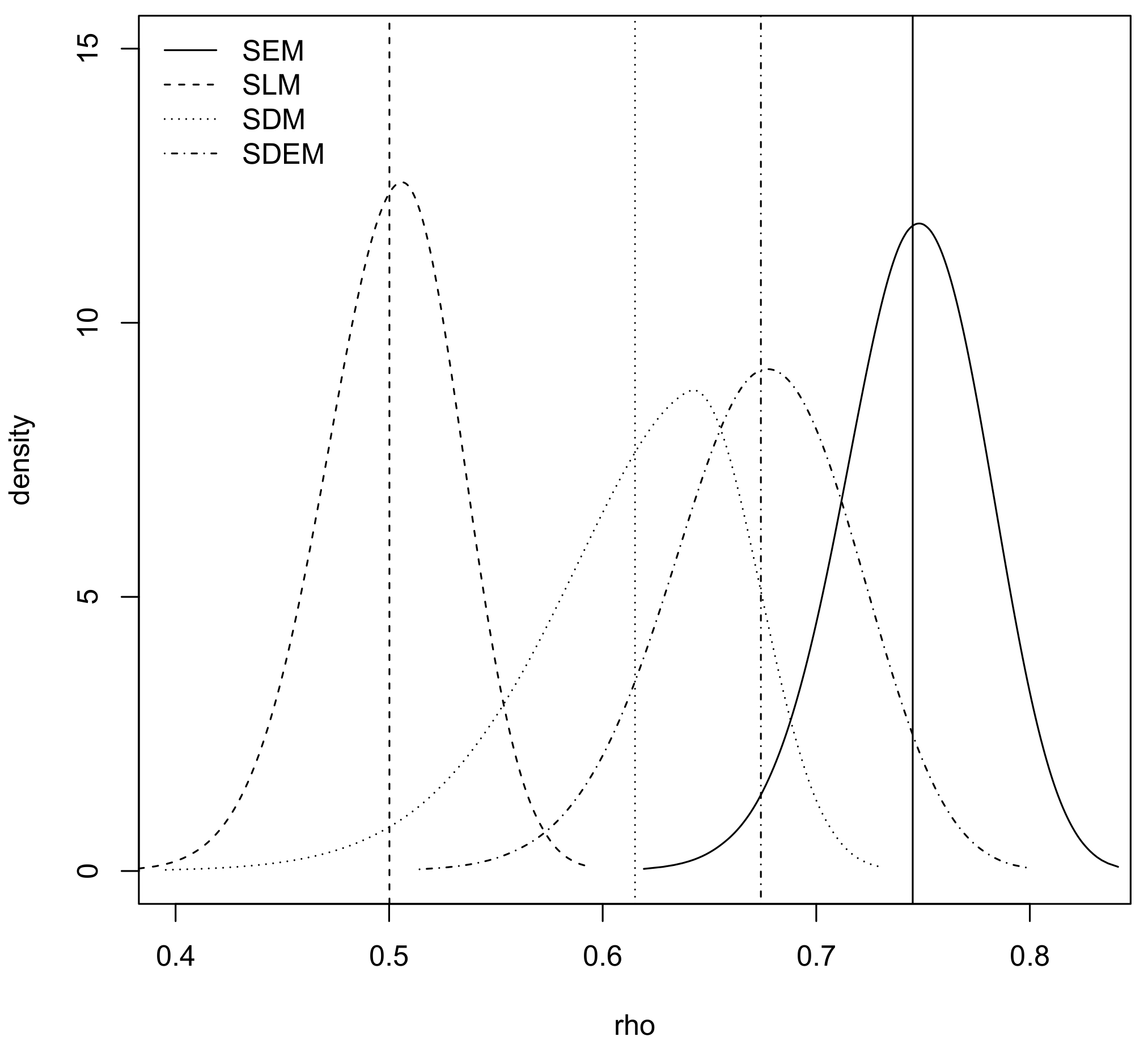
First of all, we have fitted the five models described in Section 2.1. Point estimates of the fixed effects are summarised in

Table 1. Posterior means of the fixed effects coefficients, Boston housing data.

	SEM	SLM	SDM	SDMlag	SDEM	SDEMlag	SLX	SLXlag
(Intercept)	3.542	2.168	1.946		4.364		5.122
CRIM	$-0.007$	$-0.007$	$-0.006$	$-0.003$	$-0.007$	$-0.006$	$-0.007$	$-0.015$
ZN	0.000	0.000	0.000	$-0.000$	0.000	$-0.001$	0.000	0.000
INDUS	0.001	0.002	$-0.000$	0.000	0.001	0.001	$-0.002$	0.002
CHAS1	$-0.047$	$-0.002$	$-0.062$	0.110	$-0.047$	0.133	$-0.065$	0.194
NOX^2	$-0.149$	$-0.232$	0.011	$-0.404$	$-0.050$	$-0.585$	0.081	$-1.056$
RM^2	0.010	0.008	0.010	$-0.009$	0.010	$-0.002$	0.009	$-0.007$
AGE	$-0.001$	$-0.000$	$-0.001$	0.002	$-0.001$	0.001	$-0.001$	0.002
log(DIS)	$-0.033$	$-0.140$	$-0.040$	$-0.064$	$-0.082$	$-0.076$	$-0.038$	$-0.221$
log(RAD)	0.059	0.062	0.052	$-0.004$	0.059	0.014	0.043	0.078
TAX	$-0.001$	$-0.000$	$-0.000$	0.000	$-0.000$	0.000	$-0.000$	0.000
PTRATIO	$-0.018$	$-0.013$	$-0.013$	$-0.002$	$-0.016$	$-0.016$	$-0.012$	$-0.027$
B	0.001	0.000	0.001	$-0.001$	0.000	$-0.000$	0.001	$-0.001$
log(LSTAT)	$-0.226$	$-0.218$	$-0.215$	0.054	$-0.233$	$-0.112$	$-0.234$	$-0.180$

. In addition, the posterior marginal of the spatial autocorrelation parameters are displayed in Figure 1, including posterior means. Note that these values are not the ones reported in the R-INLA output and that we have re-scaled them as explained in Section 3. In this case, the range used for the spatial autocorrelation parameter is $(-1,1)$. This will make the summary statistics for $\rho$ directly comparable to those reported in Bivand et al. [11].

In general, all our results match theirs, as expected. However, the new slm latent effects make fitting these models with R-INLA simpler. Finally, Figure 2 shows a map of the values of the slm latent effects for the SEM and SDEM.

Note that in order to fit the model, we have set the variance of the Gaussian likelihood to a fixed and tiny value (by setting the log-precision to 15) because this error term does not appear in the different spatial econometrics model fits. A side effect of this is that the DIC will be the same for all models (and it cannot be used for model comparison) and that the fitted values will also have a tiny variance. The fitted values could be computed in the right way by adding extra observations with missing values (i.e., NA) in the response; this observation will not be used for model fitting and the fitted values will now account for the required uncertainty.

7.1.1. Smoothing Covariates

So far, we have considered the squared values of NOX in our models but the relationship between this covariate and the response may take other forms. In Section 4.3, we have discussed how R-INLA implements some latent effects to smooth covariates (see, for example, Chapter 9 of [25]). One of them is the second order random walk that we have used here to smooth the values of nitric oxide concentration (parts per 10 million), which is covariate NOX. This smoother needs to be included additively in all the other effects, so it is only readily available for the SEM, SDEM and SLX model. This latent model has only one hyperparameter, which is its precision. In order to avoid overfitting and force the random walk to produce a smooth function, a gamma prior with mean 2000 and variance 10 has been used for the precision in all models, so that the level of smoothing can be compared. The results are shown in Figure 3.

SEM and SDEM show a similar linear effect, which is consistent with the findings in Harrison and Rubinfeld [29]. The SLX model seems to provide similar estimates of this effect but with considerably narrower credible intervals. As no spatial random effects are included in this model, we believe that the smoother on NOX is picking up residual spatial effects.

7.1.2. Impacts

Average direct, indirect and total impacts have been computed for the models fitted to the Boston housing data set. In addition, for the SLM and SDM, we have also fitted the models using maximum likelihood and computed their impacts for purposes of comparison. Average direct impacts, average total impacts and average indirect impacts are provided in the Supplementary Materials. Impacts are very similar between ML and Bayesian estimation for the models where we have computed them using functions in the spdep package.

Inference on the different impacts is based on their respective posterior marginal distributions provided by R-INLA. In addition to the posterior means, other statistics can be obtained, such as standard deviation, quantiles and credible intervals. These posterior marginal distributions can also be compared to assess how different models produce different impacts. Figure 4 shows the total impacts for NOX-squared under five different models. Given that for SLM and SDM we were using an approximation, we have included, with a thicker line, the distribution of the total impacts obtained with the Matlab code in the Spatial Econometrics Toolbox for these two models. The results clearly show that our approximation is very close to the results based on MCMC. Furthermore, we have checked that similar accuracy is obtained for all the covariates included in the model.

7.1.3. Prediction of Missing Values

As stated in Section 6.2.2, INLA and R-INLA can provide predictions of missing values in the response. We will use this feature to provide predictions of the 16 tracts with censored observations of the median values, treated as missing values. This will allow us to use the complete adjacency structure and to borrow information from neighbouring areas to provide better predictions.

With R-INLA, this is as simple as setting the censored values in the response to NA. We will obtain a predictive distribution for the missing values so that inference can be made from them. We have represented the five marginal distributions obtained with the models in Figure 5 for six selected areas. The vertical line shows where the censoring cuts in.

Areas 13 to 17 seem to have predicted values well below the cut-off point. These areas are located in the city centre, where house prices are likely to be higher than average and that is why our model does not predict well there. Furthermore, the predicted values of the remaining 11 areas with missing values have a similar behaviour as in Area 312 (included in Figure 5), that is, the cut-off point is close to the median of the predicted values.

Furthermore, in the Supplementary Materials, we show the posterior means of the slm latent effects for the SEM and SDEM in the same way as in Figure 2 for the incomplete data set. The main difference is that the new maps include predictions for the areas with the censored observations but the estimates in the common tracts are similar.

7.2. Business Opening after Katrina

LeSage et al. [21] studied the probabilities of re-opening a business in New Orleans in the aftermath of hurricane Katrina. They used a spatial probit, like the one described in Equation (17). Here, we reproduce the analysis with a continuous link function (i.e., a probit function) and the new slm latent model, similarly as in Bivand et al. [11].

7.2.1. Standard Models

Table 2. Summary of point estimates of the fixed effects coefficients, Katrina business data.

	SEM	SLM	SDM	SDMlag	SDEM	SDEMlag	SLX	SLXlag
(Intercept)	$-19.800$	$-8.142$	$-15.108$		$-12.775$		$-9.116$
flood_depth	$-0.434$	$-0.187$	$-0.480$	0.012	$-0.497$	0.100	$-0.323$	0.048
log_medinc	1.925	0.776	2.329	$-0.891$	2.092	$-0.887$	1.453	$-0.582$
small_size	$-0.348$	$-0.403$	$-0.431$	$-1.113$	$-0.403$	$-0.583$	$-0.287$	$-0.703$
large_size	$-0.403$	$-0.475$	$-0.372$	$-1.646$	$-0.416$	$-1.913$	$-0.242$	$-1.011$
low_status_customers	$-0.335$	$-0.480$	$-0.103$	$-1.759$	$-0.089$	$-1.620$	$-0.059$	$-1.083$
high_status_customers	0.135	0.105	0.049	0.113	0.067	0.261	0.035	0.083
owntype_sole_proprietor	0.774	0.790	0.910	1.393	0.844	0.853	0.613	0.808
owntype_national_chain	0.087	0.138	0.213	2.066	0.174	2.449	0.119	1.167
DIC	664.563	664.358	683.732		664.680		703.411
M. Lik.	$-386.500$	$-401.648$	$-435.459$		$-408.367$		$-410.769$

shows point estimates (posterior means) of the fixed effects for the five of the models discussed in Section 2.1.

Furthermore, Figure 6 shows the marginal distribution of the spatial autocorrelation parameters of four different spatial econometrics models for INLA and MCMC. For the INLA models, the values of the spatial autocorrelation parameters have been properly re-scaled to fit in the correct range and not constrained to the $(0,1)$ interval. In this example, $\rho$ could be from $-3.276$ to 1, but we have only considered it to be in the $(-1,1)$ so that a fair comparison with MCMC can be made. INLA estimates for both fixed and spatial autocorrelation estimates are very similar to those reported by Bivand et al. [11]. The posterior mean of the spatial autocorrelation for the SDM differs but this may be because Bivand et al. [11] constrained $\rho$ to be in the (0,1) interval. The SDM seems to have a weaker residual spatial correlation, probably because the inclusion of the lagged covariates reduces the autocorrelation in the response.

Regarding INLA and MCMC estimates, although the marginals are close for the SLM, they are a bit further away for all the other three models presented in Figure 6. The posterior modes are close but these differences may be due to the fact that two different link functions are used as the MCMC implementation which defines a latent continuous variable $y_i^{*}$ so that the response is 1 when $y_i^{*}$ is non-negative and 0 otherwise. This makes the models fit with INLA and MCMC differently in practice. The results obtained in the simulation study included in the Appendix A and Appendix B also support the assertion that the differences are due to the different link functions.

7.2.2. Exploring the Number of Neighbours

LeSage et al. [21] used a nearest neighbours method to obtain an adjacency matrix for the businesses in the data set. In addition, they explored the optimal number of nearest neighbours by fitting the model using different numbers of nearest neighbours and using the model with the lowest DIC [26] as the one with the optimal number of neighbours. For the 3-month horizon model, they compared a window of 8–14 neighbours, probably because of the computational burden of MCMC, which they used to fit their models.

The newly available slm in R-INLA makes exploring the optimal number of neighbours faster and simpler. We have increased the number of neighbours considered, between 5 and 35, and fitted the SLM using different adjacency matrices. These adjacency matrices have been created using the nearest neighbour algorithm with different values of the number of neighbours. Figure 7 shows how the optimal number of neighbours seems to be 22 according to both the DIC and the posterior probability (as explained in Section 6.1) criteria. However, we believe that this should be used as a guide to set the number of neighbours as there may be other factors to take into account. In particular, a nearest neighbour approach may consider as neighbours businesses that are in different parts of the city, particularly if the number of nearest neighbours is allowed to be high.

When computing the posterior probability, the prior probability of each model is taken so that $\pi \left({\mathcal{M}}_i\right)\propto 1$, and there is no prior preference on the number of neighbours. If we decide to favour adjacencies based on a small number of neighbours, we may use a more informative prior. For example, we could take $\pi \left(k\right)\propto \frac{1}{k^2}$ so that neighbourhoods with a smaller number of neighbours are preferred. Figure 7 shows the prior and posterior probability for different values of the number of neighbours. Now, it can be seen how our prior information produces different posterior probabilities, with an optimal number of neighbours of 8.

Finally, it is also possible to average over the ensemble of models using Bayesian model averaging. This will produce a fitted model that takes into account all the adjacency structures, weighted according to their marginal likelihoods.

Table 3. Summary statistics of the covariate coefficients for the model with the highest probability (under two different priors) and the BMA model (under two different priors.)

	Model with Highest Post. Prob				BMA Models
	Uniform Prior		Informative Prior		Uniform Prior		Informative Prior
	Mean	SD	Mean	SD	Mean	SD	Mean	SD
(Intercept)	$-6.831$	2.880	$-8.645$	3.086	$-7.452$	3.109	$-8.544$	3.299
flood_depth	$-0.130$	0.054	$-0.206$	0.056	$-0.155$	0.067	$-0.201$	0.070
log_medinc	0.643	0.281	0.829	0.301	0.708	0.304	0.819	0.323
small_size	$-0.409$	0.187	$-0.407$	0.186	$-0.421$	0.188	$-0.410$	0.187
large_size	$-0.419$	0.441	$-0.545$	0.449	$-0.457$	0.445	$-0.509$	0.449
low_status_customers	$-0.436$	0.207	$-0.492$	0.208	$-0.450$	0.212	$-0.497$	0.213
high_status_customers	0.099	0.171	0.124	0.171	0.108	0.172	0.107	0.172
owntype_sole_proprietor	0.805	0.262	0.757	0.262	0.788	0.262	0.772	0.262
owntype_national_chain	0.085	0.503	0.107	0.496	0.106	0.500	0.116	0.496

shows the estimates of the fixed effects for the model with the highest posterior probability according to a uniform prior ($\pi \left(k\right)\propto 1$) and an informative prior ($\pi \left(k\right)\propto 1/k^2$), and the estimates obtained by averaging over all the fitted models. These models should take into account the uncertainty about the number of neighbours and can provide different estimates of the fixed effects. As it happens, the posterior means and standard deviations are slightly different, but we can observe higher differences in the case of an informative prior.

7.2.3. Impacts

We have followed the method described in Section 5 to approximate the impacts for the models fitted to the Katrina data set. In this case, we do not have any model fitted using ML with which to compare. The implementation of the spatial probit in the Spatial Econometrics Toolbox is for a different link, so our results cannot be directly compared to MCMC, as reported by LeSage et al. [21]. Direct impacts are shown in

Table 4. Direct impacts, Katrina data set.

	INLASEM	INLASLM	INLASDM	INLASDEM	INLASLX
flood_depth	$-0.086$	$-0.038$	$-0.100$	$-0.099$	$-0.090$
log_medinc	0.381	0.159	0.504	0.409	0.386
small_size	$-0.070$	$-0.084$	$-0.097$	$-0.079$	$-0.079$
large_size	$-0.078$	$-0.100$	$-0.085$	$-0.080$	$-0.068$
low_status_customers	$-0.067$	$-0.100$	$-0.034$	$-0.018$	$-0.016$
high_status_customers	0.027	0.022	0.009	0.014	0.010
owntype_sole_proprietor	0.154	0.165	0.201	0.165	0.169
owntype_national_chain	0.016	0.025	0.060	0.033	0.033

, whilst total and indirect impacts are available in the Supplementary Materials.

Inference on the impacts relies on sampling from the approximation to the joint posterior distribution which is then used to compute the impacts and estimate their posterior distributions, as we have already seen in the Boston housing data example. Figure 8 shows the estimates of the average total impacts for flood depth for four models. With a thicker line, we have included the posterior marginal of the impacts computed using the output from MCMC using the spatialprobit package. As previously stated, MCMC results can be roughly compared to our SLM estimates but keeping in mind that different link functions have been used and that differences may appear. In this case, the quality of our approximations differs with the models. We have found similar accuracy for all the other variables, which means that our approximation appears to be acceptable.

Note that the impacts estimated with INLA and MCMC are close regardless of the estimates of the spatial autocorrelation parameters shown in Figure 6. We believe that this is because the impacts themselves build on the fitted model parameter values rather than the posterior distributions, which only enter into simulations to obtain the distributions of the impacts.

8. Discussion and Final Remarks

In this paper, we have described how the analysis of spatial econometrics data requires the use of very specific models and how the integrated nested Laplace approximation offers an alternative to model fitting. Instead of resorting to MCMC methods, INLA aims at providing approximate inference on the marginal distribution of the model parameters. This methodology is implemented in the R package R-INLA, which includes a particular latent effect called slm which can be used to fit many spatial econometrics models.

We have also shown how impacts can be approximated when models are fitted with R-INLA. As this requires multivariate posterior inference, the estimation of the impacts is achieved by sampling from the approximation to the joint posterior of the required coefficients and spatial autocorrelation parameter and computing the impacts using these samples. It is worth noting that these samples are independent, so fewer samples are required for inference than with typical MCMC algorithms.

It should be noted that there are several advantages of using INLA and R-INLA. Not only are model specification and fitting very easy using R but also the computational speed allows us to explore a large number of models. When the model is not available within the range of latent models available in R-INLA, it is often possible to fit conditional models, on one or two model parameters, and then obtain the desired model by averaging over these models. Furthermore, other important topics in Bayesian inference, such as prediction of missing responses, model selection and variable selection, can be tackled with INLA. Several authors (see, for example, [31,32]) have assessed the accuracy of INLA (as compared to MCMC) for a wide range of models, so we believe that this will also be the case for the spatial econometrics models presented herein.

In the future, we expect to explore how to increase the number of spatial econometrics models available in R-INLA and how to extend them. In particular, we find that there is interesting work to do on models with more than one spatial term, spatio-temporal models, the analysis of panel data and how to account for measurement error in covariates, for example.