Extension of SEIR Compartmental Models for Constructive Lyapunov Control of COVID-19 and Analysis in Terms of Practical Stability

Abstract

Due to the worldwide outbreak of COVID-19, many strategies and models have been put forward by researchers who intend to control the current situation with the given means. In particular, compartmental models are being used to model and analyze the COVID-19 dynamics of different considered populations as Susceptible, Exposed, Infected and Recovered compartments (SEIR). This study derives control-oriented compartmental models of the pandemic, together with constructive control laws based on the Lyapunov theory. The paper presents the derivation of new vaccination and quarantining strategies, found using compartmental models and design methods from the field of Lyapunov theory. The Lyapunov theory offers the possibility to track desired trajectories, guaranteeing the stability of the controlled system. Computer simulations aid to demonstrate the efficacy of the results. Stabilizing control laws are obtained and analyzed for multiple variants of the model. The stability, constructivity, and feasibility are proven for each Lyapunov-like function. Obtaining the proof of practical stability for the controlled system, several interesting system properties such as herd immunity are shown. On the basis of a generalized SEIR model and an extended variant with additional Protected and Quarantined compartments, control strategies are conceived by using two fundamental system inputs, vaccination and quarantine, whose influence on the system is a crucial part of the model. Simulation results prove that Lyapunov-based approaches yield effective control of the disease transmission.

1. Introduction

The COVID-19 pandemic, among other pandemics from the past, has attracted great attention not only from mathematicians but researchers from numerous fields. This is due to the fact that the exponential growth in the number of cases of infection has made the recent situation very worrying. Hence, various measures are taken for the purpose of limiting the spread of infection. Concerning COVID-19, since the extent and duration of it has lasted much longer than expected, solving the overwhelming chaos is recognized as being the most important issue in recent months. The outbreak of the pandemic has been affecting almost all countries in the world, changing people’s daily lives and causing heavy casualties. The situation calls for a dynamic model of the pandemic to analyze the system behavior. When the outbreak is in an active stage, the model should be not only descriptive, but also suitable for controller design.

1.1. Historical Development of Compartmental Models for Epidemics

In the history of mathematical models in epidemiology, the focus has always been on deterministic compartmental models, which can be defined as a sub-categorization of the whole population into different compartments, introducing transfer rates from one category to another, and modeling contact between individuals from two compartments using multiplication of the two. The works of Daniel Bernoulli (1700–1782), see [1,2], are considered as the first models and studies in mathematical epidemiology. These two pioneer works have always aroused a strong resonance in the mathematical scientific community, see, for instance, in D’Alembert [3] and Duvillard [4]. Nevertheless, the model proposed by Kermack and McKendrick [5] is the first model which takes the spread of infection into consideration. It is remarkable that the Kermack and McKendrick model can be considered as a special case of the Lotka–Volterra model of predator and prey dynamics, which was published by Lotka in 1925 [6] and by Volterra in 1926 [7]. The Lotka–Volterra equation can be used to model a pandemic, because infected people can be regarded as predators and susceptible people can be treated as a prey compartment. Setting the parameter $\alpha =0$ in the Lotka–Volterra model, which states the contact between the prey and predator in the equation characterizing the dynamics of the prey, simplifies the model to the one of Kermack and McKendrick.

According to Kermack and McKendrick [5], the original mathematical description of the spread of infectious diseases in a population is the SIR model, which separates the whole population into three parts: Susceptible (S), Infected (I) and Removed (R) compartments. However, this model is only suitable for diseases against which people can obtain permanent immunity after a short period of infection, and only for short durations of the latent stage. In the much more complicated case of COVID-19, the SEIR model is assumed to be more appropriate. The additional compartment is the group of Exposed individuals, who are in their latent state, not showing symptoms yet. Some works which utilize the SEIR model in this simple form consider individuals from compartment E to be already infectious, but most do not. To further increase the model fidelity, the SPEIQRD model has been put forward in [8], where Q represents the Quarantined, P the Protected, and D the Dead compartment. This model advances the previous one by categorizing people into more detailed compartments to analyze the complex situation. In many recent studies, researchers have proposed numerous models with a good deal of variables and parameters, aiming at making reliable predictions for the evolution of the current epidemic in spite of the limited knowledge of this specific disease and considerable uncertainty of the data collection. The common goal is to quickly estimate the impact of COVID-19 on the future of each compartment, the measures to be taken by the public health system and the effectiveness of different quarantine and vaccination measures [9].

1.2. Motivation

Compartmental models are a common tool to tackle problem formulations such as the given one, as they allow to precisely describe the transmission patterns of diseases. Based on a compartmental model, ref. [10] focuses on risk estimation and prediction while [11] puts an eye on the effect of time delay and relaxation of isolation. The aim of our study, on the other hand, is to evaluate the effectiveness of interventions, analyzing and simulating the situation in a more mathematical way. Judging from the sparsity of corresponding literature, the application of methods from the mathematical field of control to COVID-19 dynamic models still seems to be in its initial stage. Therefore, in the paper at hand, we consider both the SEIR model and the SPEIQRD model accompanied with two control actions: vaccination and quarantine, in order to estimate the spread of the virus and control the number of infected and dead people by tuning the controller. Another focus is on analyzing the stability of the closed-loop system by using the Lyapunov theory.

The Lyapunov theory is one of the most important approaches to analyze and control nonlinear systems. In the last decades, it was noticed that Lyapunov’s approaches are suitable also for constructive purposes, for overcoming concrete problems in physics and in particular in technological systems. Since then, as the growing number of publications shows, problems concerning stability and controlling dynamics can be constructively solved using this theory. Today, this theory is also used for practical tasks in the fields of mechanical and electrical engineering, especially in control engineering. The theory of Lyapunov’s direct method has been greatly promoted and brought to a certain conclusion. In the recent years, constructive results in many areas of control applications [12,13] indicate the efficacy of this theory in practical applications. Many variations of this theory appeared in the last years to make its general approach to different applications more elastic. The classical Lyapunov theory, however, sometimes is not constructive enough for practical purposes. This turns out to be the case in this contribution. Thus, practical stability [14] is considered here. Although a desired state of a given system may be mathematically unstable, the system may be permitted to oscillate around (and sufficiently near) this trajectory, which can be stipulated as acceptable. As defined in [14], if a Lyapunov-like function reaches a specific minimum point which is not equal to zero, it can still be implied that the system is practically stable. Furthermore, Moreau and Aeyels [15] describe the practical stability as a consequence of the convergence property of solutions, attaining a globally uniformly asymptotically stable equilibrium point.

In the paper at hand, the concept of practical stability is applied and plays a crucial role in the proposed solutions. The aim of this study is to achieve a practically stable system by analyzing the change of the size of Susceptible, Exposed, Infected, Recovered and Dead compartments based on the protection and contact controls, infection rate, latent period, recovery rate and mortality.

1.3. Literature Review

As shown in [16], mathematical models are a key tool for guiding public health measures in order to make decisions regarding potential economic and health interventions and when deciding how to intervene. To obtain models, a possible approach are evolutionary epidemic diffusion models [17] using suitable data, or more traditionally, compartmental models similar to the classic SEIR model, an overview of which can be found in [18]. An interesting paper is [19], where an SEIR model for COVID-19 dynamics incorporating the environment and social distancing is considered. This model indicates that disregarding social distancing and hygiene concepts can cause devastating effects on the human population. On the other hand, as shown in [20], lockdowns limited to communities together with travel restrictions are commonly employed to reduce epidemic spreading, but not totally effective if the people are not completely sealed off. In this contribution, a stochastic model on different social networks is considered to determine the level of effectiveness of lockdowns and to identify which social network compartments should be considered. A case study of the cruise ship Diamond Princess is presented in [21]. It is used as a sample population for a dedicated SEIR model that is sub-partitioned not only into symptomatic and asymptomatic infections, but also into passengers and crew members for the other compartments. Splitting or sub-partitioning compartments like this is an approach to refine the modeling depth, for finer reproduction of observed phenomena. The same is done in [22], where symptomatic and asymptomatic compartments are split again into detected and undetected compartments, respectively. In [23], the S, E, I, and A (asymptomatic) compartments are split into active and self-isolating (or social distancing) compartments for an investigation, showing how effective several different countermeasures are.

Some authors [24,25] propose to keep the model as simple as possible because of the thin data availability in early periods, with the purpose of focusing on specific local peculiarities. Simultaneously, some authors [8,26,27,28,29,30] use fractional-order models and/or controllers instead of classical integer-order calculus to model the dynamics of the compartments, at the cost of increased complexity and required computational resources, because of the infinite memory problem and other aspects. Nevertheless, to control the system using a fractional model is a new trend which can be generally justified by the chaotic nature of the considered phenomena, as already tested for other nonlinear oscillating systems.

As soon as a model is formulated with a sensible modeling depth and identified, given suitable data, it can be used to mathematically analyze the system and also predict the progression of the pandemic. The contribution [31] treats the simple SEIR model and derives analytical solutions for the compartments in case of free spread. In addition, in [32], an estimation of undetected cases based on compartmental models is presented. A system-theoretic approach is pursued in [33], where the resulting parameters are analyzed regarding the sensitivity and conditional local asymptotic stability of the equilibria is mathematically proven. In [34], the global stability is calculated using a Lyapunov function construction while the local stability is determined using a Jacobian. In [35], an interval predictor in combination with the SEIR model is proposed to predict the virus propagation in eight different countries. For this purpose, the system parameters are modeled to be time-varying and are identified using the available data, reflecting the societal reactions to the pandemic and the countermeasures. The goal of the paper [36] is to predict the system response using different values of a protection-related system parameter as control influence.

Regarding the application of methods from the field of control theory, a few papers have appeared only recently, ref. [37] being one of the first. In this work, a proportional-integral-derivative (PID) controller is applied for the first time in the context of epidemiological models. In [38], the control strategy is derived from a classical SIR epidemiological model. In this work, the vaccination rate is the control variable and chaotic behavior can be avoided by using a constant and suitably large vaccination rate. More recently [38], a vaccination based sliding mode control (SMC) strategy is designed to guarantee that the proportion of infected sub-compartments in the total compartment converges to the desired reference.

In addition, in the field of identification and modeling for the control, different papers appeared very recently, in particular in the field of network structures, including neural networks and networks of models. In [39], to help the control of the infection rate by the early identification of suspected COVID-19 cases, an algorithm which transforms the original problems into an optimization problem for a dynamic network topology is proposed. In [40], the authors analyze the limiting behavior of the SEIR model, presenting necessary and sufficient conditions for estimating the spreading parameters from data with the intention to have a tool to predict the spread of the infection.

After setting up the network of model, the selection of controllers, along with reliable data, is also a critical process, aiming at suiting national conditions. In [41], an SEIR model of city-level transmission of an infectious agent characterizes spread using different conditions: from no control to partial, from full lockdown to social distancing. Estimates of the relevant parameters of the SEIR model are obtained and the robustness of predictions under uncertainty of those estimates are shown. Possible control actions representing social, political, and medical interventions are proposed in [42]. Optimal control of COVID-19 in Ireland is treated in [43], where the cost to the economy is minimized, subject to state constraints regarding the health service capacity. The control input is realized as a piecewise-constant, time-varying infection rate, representing non-pharmaceutical interventions. In a similar contribution [44], an optimal control based on a compartmental model to steer the progression of COVID-19 is proposed. In [45], a mathematical model for COVID-19 based on an increased number of compartments is developed and stability of its equilibria is analyzed depending on the model parameters. Optimal control analysis involving a min-max optimization problem reveals that the combination of public health education, personal protective measure, and treating COVID-19 patients realizes the best control solution, obtaining the requested mitigation of transmission of the infection. Two controllers have been designed in [46]: media campaigns and treatment. By analyzing the diffusion mechanism of COVID-19, a new compartmental model and a nonlinear adaptive control problem are established. The adaptive laws are then used to update the parameters of the designed controller to achieve the goals.

1.4. Structure of the Paper

The paper is structured in the following way. Section 2.1 shows the classical SEIR model and a controller based on this. Due to problematic model behavior, an extended version is presented in Section 2.3, together with two controllers based on different Lyapunov-like function candidates. Then, Section 4 illustrates the experimental results obtained from computer simulations and Section 5 gives some concluding remarks, outlook and possible future work.

2. Methodology

Two models are described in the following subsections, representing different modeling depths and level of detail. Moreover, the derivation of the corresponding control methodology is presented. Obtaining the proof of practical stability for the closed-loop system, several interesting system properties such as herd immunity are shown.

2.1. Generalized SEIR Model

The generalized SEIR model takes Kermack and McKendrick’s SIR model as a basis and modifies it in several aspects. It is assumed that the sum of the four categories $S,E,I,R$ is equal to the total population (M) at time $t=0$ (system parameters relate to the time t in days):

$$S\left(0\right)+E\left(0\right)+I\left(0\right)+R\left(0\right)=M.$$

(1)

Then, the dynamics are

$$\begin{array}{cc}\hfill \frac{\mathrm{d}S\left(t\right)}{\mathrm{d}t}& =-\alpha I\left(t\right)\frac{S\left(t\right)}{M}+{\mu }_v\left(t\right)\hfill \\ \hfill \frac{\mathrm{d}E\left(t\right)}{\mathrm{d}t}& =\alpha I\left(t\right)\frac{S\left(t\right)}{M}-\beta E\left(t\right)-{\mu }_q\left(t\right)\hfill \\ \hfill \frac{\mathrm{d}I\left(t\right)}{\mathrm{d}t}& =\beta E\left(t\right)-\left(\gamma +\lambda \right)I\left(t\right)\hfill \\ \hfill \frac{\mathrm{d}R\left(t\right)}{\mathrm{d}t}& =\left(\gamma +\lambda \right)I\left(t\right),\hfill \end{array}$$

(2)

where the states and parameters can be interpreted as:

• $S\left(t\right)$: The number of susceptible individuals who could be potentially subjected to the infection;
• $E\left(t\right)$: The number of exposed hosts in the latent state, modeled to be not yet infectious for this model variant;
• $I\left(t\right)$: The number of infected individuals after the latent period with symptoms;
• $R\left(t\right)$: The number of removed individuals, either recovered or dead;
• $\alpha$: The infection rate, at which susceptible individuals get infected each day. $\alpha$ quantifies how many people are transitioned from $S\left(t\right)$ to $E\left(t\right)$ due to contact with $I\left(t\right)$. Since this parameter should not depend on the population size, ratio $S\left(t\right)/M$ is used in the model, so $\alpha$ has the same physical dimension as the other transition rates.
• $\beta$: Inverse of the average duration of the latent state, which turns the exposed into the infected;
• $\gamma$: The recovery rate, at which infected individuals recover ($1/\gamma$ is the average recovery time);
• $\lambda$: The death rate, at which infected individuals die ($1/\lambda$ being the average death time);
• ${\mu }_v$: Vaccination control, showing the number of susceptible individuals vaccinated per day (represented using negative signal values);
• ${\mu }_q$: Quarantine control, showing the number of susceptible individuals quarantined per day (represented using positive signal values).

Without doubt, the current situation of the pandemic is expected to stop and sustain an acceptable number of susceptible individuals. In this sense, it is useful to regard an acceptable number of Susceptibles as a minimum immunity level, $S_d$. To this goal, it is necessary to determine, coordinate and stabilize the error between the desired setpoints as the balance points of the whole population and the actual values represented by the current levels of Susceptible, Exposed and Infected individuals. This is explored through application of the direct method of Lyapunov. With zero being the intended value of $E\left(t\right)$ and $I\left(t\right)$, $S_d$ is the desired value of $S\left(t\right)$.

2.2. Analysis and Control of the Generalized SEIR Model

A possible problem formulation can be stated in the following way:

Problem 1.

Given the underactuated system defined in Equation (2), find two control laws $u_v\left(t\right)$ and $u_q\left(t\right)$ which reduce both states $I\left(t\right)$ and $E\left(t\right)$ to zero and allow $S\left(t\right)$ to reach an acceptable number $S_d$.

The so-formulated problem can be solved using the results offered by the following Theorem.

Theorem 1.

Let us consider the underactuated system defined in Equation (2) and let $S_d$ be the target for compartment $S\left(t\right)$ which guarantees the acceptable immunity in a given population M, then, there exist two control laws ${\mu }_q\left(t\right)$ and ${\mu }_v\left(t\right)$ which guarantee the asymptotical stability to zero of the Infected and Exposed compartments and a finite time convergence of the Susceptibles, respectively.

Proof. 

In order to reduce the error, let us define the following Lyapunov function candidate:

$$V_1(S,E,I)=\frac{1}{2}{\left(S\left(t\right)-S_d\right)}^2+\frac{1}{2}E{\left(t\right)}^2+\frac{1}{2}I{\left(t\right)}^2.$$

(3)

It is enough for asymptotical stability to obtain

$${\dot{V}}_1(S,E,I)<0,$$

(4)

if this is true then the desired equilibrium can be reached. By differentiating the function, we obtain $\dot{V_1}$:

$$\begin{array}{cc}\hfill \dot{V_1}(S,E,I)& =\left(S\left(t\right)-S_d\right)\dot{S}\left(t\right)+E\left(t\right)\dot{E}\left(t\right)+I\left(t\right)\dot{I}\left(t\right)\hfill \\ \hfill & =\left(S\left(t\right)-S_d\right)\left(-\frac{\alpha }{M}I\left(t\right)S\left(t\right)+{\mu }_v\left(t\right)\right)\hfill \\ \hfill & +E\left(t\right)\left(\frac{\alpha }{M}I\left(t\right)S\left(t\right)-\beta E\left(t\right)-{\mu }_q\left(t\right)\right)\hfill \\ \hfill & +I\left(t\right)\left(\beta E\left(t\right)-\left(\gamma +\lambda \right)I\left(t\right)\right).\hfill \end{array}$$

(5)

In order to obtain ${\dot{V}}_1(S,E,I)=0$, the following two equivalent control laws can be obtained

$$\begin{array}{cc}\hfill {\mu }_{eqv}\left(t\right)& =\frac{\alpha }{M}I\left(t\right)S\left(t\right),\hfill \end{array}$$

(6)

$$\begin{array}{cc}\hfill {\mu }_{eqq}\left(t\right)& =\frac{\alpha }{M}I\left(t\right)S\left(t\right)-\beta E\left(t\right).\hfill \end{array}$$

(7)

Inspired by the sliding mode control (SMC) approach, we add a corrective part to the two control laws, in which ${\eta }_{v,q}>0$, with the goal to stabilize the error dynamics:

$$\begin{array}{cc}\hfill {\mu }_v\left(t\right)& ={\mu }_{eqv}\left(t\right)-{\eta }_v\mathrm{sgn}\left(S\left(t\right)-S_d\right),\hfill \end{array}$$

(8)

$$\begin{array}{cc}\hfill {\mu }_q\left(t\right)& ={\mu }_{eqq}\left(t\right)+{\eta }_q\mathrm{sgn}\left(E\left(t\right)\right).\hfill \end{array}$$

(9)

Let us consider the following part of the model:

$$\begin{array}{cc}\hfill \frac{\mathrm{d}S\left(t\right)}{\mathrm{d}t}& =-\alpha I\left(t\right)\frac{S\left(t\right)}{M}+{\mu }_v\left(t\right)\hfill \end{array}$$

(10)

$$\begin{array}{cc}\hfill \frac{\mathrm{d}E\left(t\right)}{\mathrm{d}t}& =\frac{\alpha }{M}I\left(t\right)S\left(t\right)-\beta E\left(t\right)-{\mu }_q\left(t\right)\hfill \end{array}$$

(11)

with the control laws as defined, in which $S\left(0\right)-S_d>0$, the following dynamics are obtained:

$$\begin{array}{cc}\hfill \frac{\mathrm{d}S\left(t\right)}{\mathrm{d}t}& =-{\eta }_v\mathrm{sgn}\left(S\left(t\right)-S_d\right),\hfill \end{array}$$

(12)

$$\begin{array}{cc}\hfill \frac{\mathrm{d}E\left(t\right)}{\mathrm{d}t}& =-{\eta }_q\mathrm{sgn}\left(E\left(t\right)\right).\hfill \end{array}$$

(13)

There exist finite times $t_{S,E}^{☆}$ depending on ${\eta }_{v,q}$ such that $S\left(t_S^{☆}\right)=S_d$ and $S\left(t_E^{☆}\right)=0$:

$$\begin{array}{cc}\hfill t_S^{☆}& =\frac{S\left(0\right)-S_d}{{\eta }_v},\hfill \end{array}$$

(14)

$$\begin{array}{cc}\hfill t_E^{☆}& =\frac{E\left(0\right)}{{\eta }_q}.\hfill \end{array}$$

(15)

If ${\eta }_v>0$ and ${\eta }_q>0$, inserting the control laws into ${\dot{V}}_1(S,E,I)$ yields

$${\dot{V}}_1(S,E,I)=-{\eta }_v\left|S\left(t\right)-S_d\right|-{\eta }_q\left|E\left(t\right)\right|+I\left(t\right)\left(\beta E\left(t\right)-\left(\gamma +\lambda \right)I\left(t\right)\right).$$

(16)

Considering system model parameters $\gamma >0$ and $\lambda >0$ and the fact that $S\left(t\right)$ and $E\left(t\right)$ converge in finite time, this simplifies to

$$-I{\left(t\right)}^2\left(\gamma +\lambda \right)<0,$$

(17)

which is always true for $I\left(t\right)\ne 0$. Concluding the proof, ${\dot{V}}_1(S,E,I)<0$ or, when all errors have converged and the goal $V_1(S,E,I)=0$ is achieved, it remains at ${\dot{V}}_1(S,E,I)=0$. □

However, there is still considerable ambiguity with regard to this relatively simple model. The model neglects the contacts between exposed individuals, who do not show symptoms but are also able to spread the virus, and susceptible individuals. It also considers in the model equations a constant population size M, which is not true for this incarnation of the SEIR model, due to inputs ${\mu }_{v,q}$ that influence only single dynamics, respectively, and not in a balanced/conservative way that preserves the total population size. Moreover, owing to the complex disease, recovered people can become susceptible again, which is not covered by this simplistic model. Other aspects such as temporary isolation and a Quarantined (Q) or Protected compartment (P) are also not explicitly considered in the simple SEIR model, which leads to a total population size M that is not constant. Thus, a more detailed and specific model is proposed so as to get closer to the reality which can solve the open issues left until now.

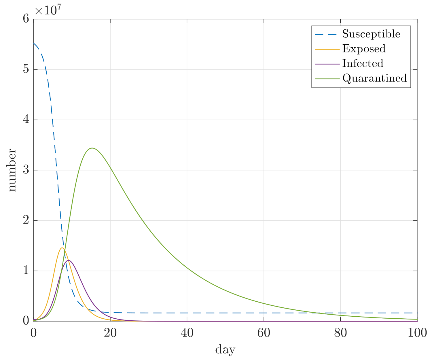
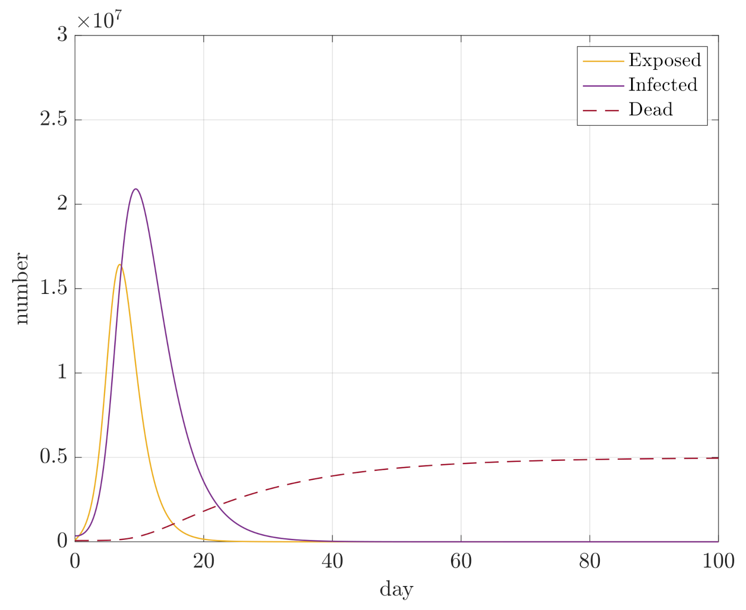
2.3. Advanced SPEIQRD Model

Considering the drawbacks of the approach proposed in the previous section, let us introduce the following modified model:

$$\begin{array}{cc}\hfill \frac{\mathrm{d}S\left(t\right)}{\mathrm{d}t}& =-\alpha \left(I\left(t\right)+E\left(t\right)\right)\frac{S\left(t\right)}{M}-\zeta \left(t\right)S\left(t\right)+\varphi R\left(t\right)\hfill \\ \hfill \frac{\mathrm{d}P\left(t\right)}{\mathrm{d}t}& =\zeta \left(t\right)S\left(t\right)\hfill \\ \hfill \frac{\mathrm{d}E\left(t\right)}{\mathrm{d}t}& =\alpha \left(I\left(t\right)+E\left(t\right)\right)\frac{S\left(t\right)}{M}-\beta E\left(t\right)\hfill \\ \hfill \frac{\mathrm{d}I\left(t\right)}{\mathrm{d}t}& =\beta E\left(t\right)-\delta \left(t\right)I\left(t\right)-\left({\gamma }_1+{\lambda }_1\right)I\left(t\right)\hfill \\ \hfill \frac{\mathrm{d}Q\left(t\right)}{\mathrm{d}t}& =\delta \left(t\right)I\left(t\right)-\left({\gamma }_2+{\lambda }_2\right)Q\left(t\right)\hfill \\ \hfill \frac{\mathrm{d}R\left(t\right)}{\mathrm{d}t}& ={\gamma }_{1}I\left(t\right)+{\gamma }_{2}Q\left(t\right)-\varphi R\left(t\right)\hfill \\ \hfill \frac{\mathrm{d}D\left(t\right)}{\mathrm{d}t}& ={\lambda }_{1}I\left(t\right)+{\lambda }_{2}Q\left(t\right).\hfill \end{array}$$

(18)

Based on the generalized SEIR model, some new variables and parameters are added or modified, as well as building up more realistic relationships between the two controllers and each category.

Remark 1.

In contrast to the SEIR model, the total population size

$$M=S\left(t\right)+P\left(t\right)+E\left(t\right)+I\left(t\right)+R\left(t\right)+Q\left(t\right)+D\left(t\right)$$

(19)

remains constant, which is due to the fact that the inputs structurally act no longer “dissipatively”, but mirrored or anti-symmetric: both inputs $\zeta \left(t\right)$, $\delta \left(t\right)$ appear in two places in the model, with opposite signs. This is obvious when considering Equation (19): differentiating this equation, we obtain that the sum of the dynamics is equal to zero, which indicates conservation of the population. Another point of view is that the inputs of the simple SEIR model (which is affine in the inputs) are external, while those of the modified model (being multiplicative in the inputs) are internal.

The parameters and states are:

• $E\left(t\right)$: The number of exposed hosts in the latent state, modeled to already be infectious for this model variant;
• $P\left(t\right)$: The number of protected individuals who have been vaccinated;
• $Q\left(t\right)$: The number of quarantined individuals who get quarantined when they are infectious;
• $R\left(t\right)$: The number of recovered individuals;
• $D\left(t\right)$: The number of dead individuals;
• $\zeta \left(t\right)$: The protection rate, at which susceptible individuals get vaccinated;
• $\varphi$: The recurrence rate, at which recovered people become susceptible again. Since the probability is tiny, we assume this parameter to be zero;
• $\delta \left(t\right)$: The quarantine rate, at which infected people get quarantined;
• ${\gamma }_2$: The recovery rate, at which quarantined individuals recover;
• ${\gamma }_1$: At this recovery rate, those infected individuals recover before quarantine. We assume the parameter to be zero since the probability is much smaller than ${\gamma }_2$;
• ${\lambda }_2$: The death rate, at which quarantined individuals die;
• ${\lambda }_1$: At this death rate, those infected individuals die before quarantine. We assume the parameter also to be zero since the probability is much smaller than ${\lambda }_2$.

2.4. Analysis and Control of the Advanced SPEIQRD Model

The improved model proposed in Equation (18) is no longer linear in the inputs, complicating the task to control, but it is possible to consider a similar problem formulation as before:

Problem 2.

Given the underactuated system defined in Equation (18), find two control laws $\zeta \left(t\right)$ and $\delta \left(t\right)$ that asymptotically reduce states $I\left(t\right)$, $E\left(t\right)$ to zero and $S\left(t\right)$ to a desired $S_d$.

Theorem 2.

Let us consider the underactuated system defined in Equation (18), together with a Lyapunov-like function candidate $V_2$ that is the same as Lyapunov function $V_1$ candidate, as in Theorem 1:

$$V_2(S,E,I)=\frac{1}{2}{\left(S\left(t\right)-S_d\right)}^2+\frac{1}{2}E{\left(t\right)}^2+\frac{1}{2}I{\left(t\right)}^2,$$

(20)

then, there exist two control laws $\zeta \left(t\right)$ and $\delta \left(t\right)$ which guarantee the asymptotical convergence of the Infected and Exposed compartments to zero, and the Susceptibles to a suitable immunity level, if the following sufficient conditions are met:

$$\begin{array}{cc}\hfill {\eta }_q& >\frac{E\left(t\right)\alpha \left(I\left(t\right)+E\left(t\right)\right)\frac{S\left(t\right)}{M}+\beta E\left(t\right)I\left(t\right)}{I{\left(t\right)}^2},\hfill \end{array}$$

(21)

$$\begin{array}{cc}\hfill {\eta }_v& >\frac{\alpha E{\left(t\right)}^2}{M\left|S\left(t\right)-S_d\right|},\hfill \end{array}$$

(22)

$$\begin{array}{cc}\hfill S_d& <\frac{\beta M}{\alpha }.\hfill \end{array}$$

(23)

Remark 2.

Classical Lyapunov functions contain all the system states (or to be more precise in a control context, the corresponding state variables’ errors)—$V_2$ does not, rendering it a Lyapunov-like function candidate. Stability analyses using Lyapunov-like functions are called practical stability analyses and usually require a more in-depth investigation than the classic Lyapunov theory. On the other hand, choosing a classical Lyapunov function not only is an implicit constraint regarding the constructivity of the control law, but can also complicate the stability analysis in case of large number of states. Willingly neglecting some states in the Lyapunov function, diverging from conventional Lyapunov theory, will introduce the need to do a posteriori analyses regarding these state variables, but can significantly simplify the derivation of the results.

Proof. 

The goal is to find two control laws $\zeta \left(t\right)$ and $\delta \left(t\right)$ such that

$${\dot{V}}_2(S,E,I)<0,$$

(24)

i.e., guaranteeing convergence of the three errors to zero, and additionally showing that non-considered states also converge. By differentiating the function, we obtain ${\dot{V}}_2(S,E,I)$ as

$$\begin{array}{cc}\hfill {\dot{V}}_2& =\left(S\left(t\right)-S_d\right)\dot{S}\left(t\right)+E\left(t\right)\dot{E}\left(t\right)+I\left(t\right)\dot{I}\left(t\right)\hfill \\ \hfill & =\left(S\left(t\right)-S_d\right)\left(-\alpha \left(I\left(t\right)+E\left(t\right)\right)\frac{S\left(t\right)}{M}-\zeta \left(t\right)S\left(t\right)\right)\hfill \\ \hfill & +E\left(t\right)\left(\alpha \left(I\left(t\right)+E\left(t\right)\right)\frac{S\left(t\right)}{M}-\beta E\left(t\right)\right)\hfill \\ \hfill & +I\left(t\right)\left(\beta E\left(t\right)-\delta \left(t\right)I\left(t\right)\right).\hfill \end{array}$$

(25)

In order to reach ${\dot{V}}_2(S,E,I)<0$, consider the following two non-singular, approximate equivalent control laws

$$\begin{array}{cc}\hfill \zeta \left(t\right)& =-\frac{\alpha }{M}\left(I\left(t\right)+E\left(t\right)\right)+{\eta }_v\mathrm{sgn}\left(S\left(t\right)-S_d\right),\hfill \end{array}$$

(26)

$$\begin{array}{cc}\hfill \delta \left(t\right)& =\frac{\beta E\left(t\right)}{I\left(t\right)+1}+{\eta }_q,\hfill \end{array}$$

(27)

in which ${\eta }_{v,q}>0$. In $\delta \left(t\right)$, the denominator is chosen as $I\left(t\right)+1$ in order to approximately cancel out the factor $I\left(t\right)$ while avoiding singularities. In addition, this control law does not include a switching function as it is not required to get $\dot{V_2}<0$. Considering the inputs $\zeta \left(t\right)$ and $\delta \left(t\right)$ within the dynamics of $S\left(t\right)$, for example, yields

$$\dot{S}\left(t\right)=-{\eta }_v\mathrm{sgn}\left(S\left(t\right)-S_d\right)S\left(t\right),$$

(28)

which is an exponentially decreasing state evolution, converging to $S_d$. However, to demonstrate stability, it is sensible to insert the inputs $\zeta \left(t\right)$ and $\delta \left(t\right)$ into ${\dot{V}}_2$, to obtain the condition

$$\begin{array}{cc}\hfill \dot{V_2}& =-{\eta }_v\left|S\left(t\right)-S_d\right|S\left(t\right)\hfill \\ \hfill & +E\left(t\right)\left(\alpha \left(I\left(t\right)+E\left(t\right)\right)\frac{S\left(t\right)}{M}-\beta E\left(t\right)\right)\hfill \\ \hfill & +\beta E\left(t\right)I\left(t\right)\left(1-\frac{I\left(t\right)}{I\left(t\right)+1}\right)-{\eta }_{q}I{\left(t\right)}^2<0.\hfill \end{array}$$

(29)

In order to simplify the investigation, it is possible to consider a more conservative expression based on $\dot{V_2}$, where some terms $\le 0$ are discarded:

$${\dot{V}}_{2a}=E\left(t\right)\alpha \left(I\left(t\right)+E\left(t\right)\right)\frac{S\left(t\right)}{M}+\beta E\left(t\right)I\left(t\right)-{\eta }_{q}I{\left(t\right)}^2.$$

(30)

Using this, a condition for ${\eta }_q$ can be found that, together with another condition for ${\eta }_v$ and one for the target size of the Susceptibles compartment $S_d$, guarantees $\dot{V_2}<0$:

$${\eta }_q>\frac{E\left(t\right)\alpha \left(I\left(t\right)+E\left(t\right)\right)\frac{S\left(t\right)}{M}+\beta E\left(t\right)I\left(t\right)}{I{\left(t\right)}^2},$$

(31)

while $I\left(t\right)>0$. As soon as $I\left(t\right)=0$ is reached, the choice of ${\eta }_q$ is irrelevant. When considering $I\left(t\right)=0$, the original condition becomes

$$\dot{V_2}=-{\eta }_v\left|S\left(t\right)-S_d\right|S\left(t\right)+E{\left(t\right)}^2\left(\alpha \frac{S\left(t\right)}{M}-\beta \right)<0,$$

(32)

or, thanks to $S\left(t\right)\ge 0$ and using another more conservative expression again (neglecting negative part involving $\beta$),

$${\dot{V}}_{2b}=-{\eta }_v\left|S\left(t\right)-S_d\right|+E{\left(t\right)}^2\frac{\alpha }{M}<0$$

(33)

and, finally,

$${\eta }_v>\frac{\alpha E{\left(t\right)}^2}{M\left|S\left(t\right)-S_d\right|},$$

(34)

as long as $S\left(t\right)$ has not reached $S_d$ yet. (When $S_d$ is reached, the choice of ${\eta }_v$ is irrelevant.) Considering again Equation (32), assuming $S\left(t\right)=S_d$, the condition simplifies to

$$\dot{V_2}=E{\left(t\right)}^2\left(\alpha \frac{S_d}{M}-\beta \right)<0,$$

(35)

so

$$S_d<\frac{\beta M}{\alpha }.$$

(36)

□

Remark 3.

Note that condition (36) can be seen as a level of herd immunity, since it relates to the case where the control laws have no more influence on the system (due to their multiplicative nature in combination with variables that are already zero in the model equations). Similar conditions regarding herd immunity, derived from compartmental models, are given in [47] and, numerically, in [48].

Remark 4.

While the given conditions for ${\eta }_q$, ${\eta }_v$ and $S_d$ together are sufficient to guarantee $\dot{V_2}<0$ and thus asymptotical convergence of the considered errors to zero in all circumstances compatible with the conditions, they are not necessary and rather conservative. In fact, condition (31) alone is able to achieve the overall convergence if E and S converge faster than I does. Condition (34), on the other hand, is sufficient in case S is the slowest compartment to converge. The third condition (36) about $S_d$ is sufficient if both I and S converge faster than E. If E is the slowest compartment to converge, that is, in case $I=0$ and $S=S_d$, Equation (36) states the condition for convergence of the remaining compartment E. Depending on which state converges the slowest, in a mathematical sense it is enough to employ only one of the three sufficient conditions, but using all three (if possible) obviously speeds up convergence to our real-life goal.

In addition, the Lyapunov-like function $V_2$ already is not an orthodox choice for the system described by Equation (18) as it does not include all states, as is the case in classic Lyapunov theory, but only the states whose deviation from a reference could be seen as problematic in the given application (so S, E, and I). In fact, considering the compartment S in the Lyapunov-like function is not required in order to reach the actual real-life goal of eradicating the disease or establishing enough immunity. If one of these is achieved, it does not matter which portion of the population is still susceptible. Using the advanced model (18), other compartments are available that hold a much more direct connection to the abstract real-life goals. Thus, a more constructive Lyapunov-like approach can be found by considering the compartments P, R, E, and I. The goal is to maximize the sum of P (Protected) and R (Recovered), bringing them as close to the total population size M as possible, which means with as few D (Deaths) as possible, while at the same time forcing E and I to zero. In this sense, the following Theorem states a more suitable approach.

Theorem 3.

Let us consider the underactuated system defined in Equation (18), together with the following new Lyapunov-like function candidate:

$$V_3(P,R,E,I)=\frac{1}{2}{\left(M-P\left(t\right)-R\left(t\right)\right)}^2+\frac{1}{2}E{\left(t\right)}^2+\frac{1}{2}I{\left(t\right)}^2,$$

(37)

then, there exist two control laws $\zeta \left(t\right)$ and $\delta \left(t\right)$ which guarantee the asymptotical convergence of the Infected and Exposed compartments to zero.

Proof. 

The derivative ${\dot{V}}_3(P,R,E,I)$ is as follows:

$${\dot{V}}_3(P,R,E,I)=\left(M-P\left(t\right)-R\left(t\right)\right)\left(-\dot{P}\left(t\right)-\dot{R}\left(t\right)\right)+E\left(t\right)\dot{E}\left(t\right)+I\left(t\right)\dot{I}\left(t\right).$$

(38)

Inserting the state dynamics leads to

$$\begin{array}{cc}\hfill {\dot{V}}_3& =\left(M-P\left(t\right)-R\left(t\right)\right)\left(-\zeta \left(t\right)S\left(t\right)-{\gamma }_{2}Q\left(t\right)\right)\hfill \\ \hfill & +E\left(t\right)\left(\alpha \left(I\left(t\right)+E\left(t\right)\right)\frac{S\left(t\right)}{M}-\beta E\left(t\right)\right)\hfill \\ \hfill & +I\left(t\right)\left(\beta E\left(t\right)-\delta \left(t\right)I\left(t\right)\right).\hfill \end{array}$$

(39)

Compensating parts of each dynamics, the control laws again consist of equivalent control parts together with robustifying corrective parts similar to SMC, in which ${\eta }_{v,q}>0$:

$$\begin{array}{cc}\hfill \zeta \left(t\right)& =-\frac{{\gamma }_{2}Q\left(t\right)}{S\left(t\right)+1}+{\eta }_v\mathrm{sgn}\left(M-P\left(t\right)-R\left(t\right)\right),\hfill \end{array}$$

(40)

$$\begin{array}{cc}\hfill \delta \left(t\right)& =\frac{\beta E\left(t\right)}{I\left(t\right)+1}+{\eta }_q.\hfill \end{array}$$

(41)

By inserting the control laws into ${\dot{V}}_3$, we can obtain a condition for reaching ${\dot{V}}_3(P,R,E,I)<0$:

$$\begin{array}{cc}\hfill {\dot{V}}_3& =\left(M-P\left(t\right)-R\left(t\right)\right)[{\gamma }_{2}Q\left(t\right)\left(\frac{S\left(t\right)}{S\left(t\right)+1}-1\right)\hfill \\ \hfill & -{\eta }_{v}S\left(t\right)\mathrm{sgn}\left(M-P\left(t\right)-R\left(t\right)\right)]\hfill \\ \hfill & +E\left(t\right)\left(\alpha \left(I\left(t\right)+E\left(t\right)\right)\frac{S\left(t\right)}{M}-\beta E\left(t\right)\right)\hfill \\ \hfill & +I\left(t\right)\left(\beta E\left(t\right)\left(1-\frac{I\left(t\right)}{I\left(t\right)+1}\right)-{\eta }_{q}I\left(t\right)\right)<0.\hfill \end{array}$$

(42)

For increased readability, a new symbol ${\Delta }_{MPR}$ can be introduced:

$${\Delta }_{MPR}=\left(M-P\left(t\right)-R\left(t\right)\right){\gamma }_{2}Q\left(t\right)\left(\frac{S\left(t\right)}{S\left(t\right)+1}-1\right).$$

(43)

Since $\frac{S\left(t\right)}{S\left(t\right)+1}<1$ and $M-P\left(t\right)-R\left(t\right)>0$, ${\Delta }_{MPR}$ is always negative and does not have to be considered in the following. Including it in the calculation could potentially yield a less conservative condition, but considering that $\frac{S\left(t\right)}{S\left(t\right)+1}\approx 1$ for the most part of the reaching phase, ${\Delta }_{MPR}$ is relatively small and can be neglected without much increase in conservativeness. Thanks to this, similar to the previous approach, it is possible to find a more conservative condition by neglecting some terms $\le 0$:

$${\dot{V}}_{3a}=\alpha \left(I\left(t\right)+E\left(t\right)\right)E\left(t\right)\frac{S\left(t\right)}{M}+\beta E\left(t\right)I\left(t\right)-{\eta }_{q}I{\left(t\right)}^2<0.$$

(44)

From this, a sufficient condition for ${\eta }_q$ can be derived as

$${\eta }_q>\frac{\beta E\left(t\right)I\left(t\right)+\alpha \left(I\left(t\right)+E\left(t\right)\right)E\left(t\right)\frac{S\left(t\right)}{M}}{I{\left(t\right)}^2},$$

(45)

while $I\left(t\right)>0$. As soon as $I\left(t\right)=0$ is reached, the choice of ${\eta }_q$ is irrelevant and ${\eta }_v$ must be additionally considered, using another simplified condition stemming from ${\dot{V}}_3$:

$${\dot{V}}_{3b}=-{\eta }_{v}S\left(t\right)\mathrm{sgn}\left|M-P\left(t\right)-R\left(t\right)\right|+\alpha E{\left(t\right)}^2\frac{S\left(t\right)}{M}<0.$$

(46)

The resulting condition for ${\eta }_v$ then is

$${\eta }_v>\frac{\alpha E{\left(t\right)}^2\frac{S\left(t\right)}{M}}{S\left(t\right)\mid M-P\left(t\right)-R\left(t\right)\mid },$$

(47)

as long as $S\left(t\right)\ne 0$. When both $S\left(t\right)=0$ and $I\left(t\right)=0$ are reached thanks to adherence to conditions (45,47), the original condition simplifies to

$${\dot{V}}_3=-{\gamma }_{2}Q\left(t\right)\left(M-P\left(t\right)-R\left(t\right)\right)-\beta E{\left(t\right)}^2<0,$$

(48)

which is always true. □

Remark 5.

Conditions (45,47) are time-dependent expressions that can be evaluated for any state of the system. However, for constructive control design, worst case considerations can be done, introducing even more conservativeness

$${\eta }_q>\max \left(\frac{\beta E\left(t\right)I\left(t\right)+\alpha \left(I\left(t\right)+E\left(t\right)\right)E\left(t\right)\frac{S\left(t\right)}{M}}{I{\left(t\right)}^2}\right),$$

(49)

which obviously means $I=1$, $S=1$, $E=M-1$, yielding an even more conservative condition

$${\eta }_q>\beta E+\frac{\alpha }{M}\left(1+E\right)E.$$

(50)

A similar worst-case investigation can be done for ${\eta }_v$.

Remark 6.

Regarding the stability in practice, in the experiments section, it is shown that significantly lower values of ${\eta }_{v,q}$ than dictated from the conditions mentioned above achieve convergence, due to the fact that the conditions are rather conservative and not necessary. Nevertheless, the control laws based on $V_3$ result to be the least conservative of those investigated. Like $V_2$, function $V_3$ isnota Lyapunov function in the classic sense since it can never achieve zero, due to the term ${(M-P\left(t\right)-R\left(t\right))}^2$. M consists of the sum of all modeled compartments, $M=S\left(t\right)+P\left(t\right)+E\left(t\right)+I\left(t\right)+Q\left(t\right)+R\left(t\right)+D\left(t\right)$, so evaluating this yields a residual ${(S\left(t\right)+E\left(t\right)+I\left(t\right)+Q\left(t\right)+D\left(t\right))}^2$. While S, E, I (and, in consequence, Q) converge to zero, the D compartment cannot be decreased and remains in $V_3$.

3. Model Validation

In order to validate the quantitative prediction capabilities of the model given in Equation (18), limited though they may be, we consider the model parameters given in [49], which utilizes an SEIR model that is comparable to ours, within a well-identified sample scenario. The following shared characteristics of compartmental models are particularly important for COVID modeling: exposed patients are assumed to be infectious, there is the effect of temporary immunity, and quarantining action is modeled as well. In order to compare, we took the data from Tables 4 and 5 at page 1671 in [49] and adapted them to fit our situation, using the following changes, where the index${}_{ours}$ indicates the parameters’ symbols as used in our compartmental structure, and the right sides of the equations correspond to the symbols used in [49]:

$$\begin{array}{cc}\hfill S_{ours}\left(0\right)& =9.5\times {10}^4,\hfill \end{array}$$

(51)

$$\begin{array}{cc}\hfill {\alpha }_{ours}& ={\beta }_1+{\beta }_2+\chi ,\hfill \end{array}$$

(52)

$$\begin{array}{cc}\hfill {\beta }_{1,ours}& ={\theta }_1+{\theta }_2,\hfill \end{array}$$

(53)

$$\begin{array}{cc}\hfill {\gamma }_{1,ours}& =3\left({\gamma }_1+{\gamma }_2\right),\hfill \end{array}$$

(54)

$$\begin{array}{cc}\hfill {\gamma }_{2,ours}& =\varphi (\mathrm{set}\mathrm{to}0.1),\hfill \end{array}$$

(55)

$$\begin{array}{cc}\hfill {\delta }_{ours}\left(t\right)& =\phi (\mathrm{set}\mathrm{to}0.4)\hfill \end{array}$$

(56)

$$\begin{array}{cc}\hfill {\lambda }_{1,2,ours}& =0,\hfill \end{array}$$

(57)

$$\begin{array}{cc}\hfill {\zeta }_{ours}\left(t\right)& =0,\hfill \end{array}$$

(58)

$$\begin{array}{cc}\hfill {\varphi }_{ours}& =\alpha .\hfill \end{array}$$

(59)

The data correspond to the period from January 2020 to July 2020 in the Hubei province. In Figure 1, a simulation of the compartments of system (18) using the parameters given above is shown, to be compared with Figure 13 at page 1679 [49]. Discrepancies between the two models stem from a slightly different compartmental structure and require adjustment of some of the rates, as given above, in order to obtain some degree of comparability, even in the presence of nonlinearities. In the simulation, we can see a good match between all compartments, apart from differences in the evolution of the Infected compartment. The model proposed in [49] considers two separate compartments for the Infected and differentiates between Quarantined (Q) and Hospitalized (H) patients, while the contribution at hand uses only one compartment for the Infected and treats the Hospitalized like the Quarantined. Therefore, by comparing the sum of $I_{1,2}$ of [49] with I, we can see a good matching of the predictive capabilities of our proposed model along with that in [49].

4. Simulation Results

The simulation results for the SPEIQRD model with both approaches $V_{2,3}$ can be seen in Figure 2, Figure 3, Figure 4, Figure 5, Figure 6, Figure 7, Figure 8, Figure 9, Figure 10, Figure 11 and Figure 12. They are obtained using Matlab/Simulink computer simulations, using the system model parameters as detailed in

Table 1. Parameters.

Parameter or Variable	Value
M	60,359,546
$S\left(0\right)$	55,223,559
$P\left(0\right)$	2,215,504
$E\left(0\right)$	100,000
$I\left(0\right)$	355,983
$Q\left(0\right)$	118,661
$R\left(0\right)$	2,274,400
$D\left(0\right)$	71,439
$\alpha /M$	$1.657\times {10}^{-8}$
$\alpha$	1
$\beta$	$0.5$
${\gamma }_1$	0
${\gamma }_2$	$0.05$
${\lambda }_1$	0
${\lambda }_2$	$5\times {10}^{-3}$
$\varphi$	0
${\eta }_v$	10
${\eta }_q$	1

. The parameter values were taken from the literature [50] and complemented using guesses and plausibility considerations. In this sense, the simulation study has limited validity in terms of quantitative pandemic predictions, but it still allows to analyze the system stability as well as trends using different control strategies.

In Figure 2, all signals are displayed. In order to investigate how these two methods affect the advanced SPEIQRD model, we use Simulink to compare different results we obtained by using $V_2$ and $V_3$, showing different interpretations of each compartment and controller.

After comparing the numbers of Susceptibles, Exposed, Infected and Quarantined in Figure 3 and Figure 4, it is interesting to note that the number of the Susceptibles will reach our intended value (which is inherently zero in case of $V_3$) much faster by using $V_3$ than $V_2$, which is what was expected.

Although the sizes of Recovered and Dead compartments do not show much variation between Figure 5 and Figure 6, what we can note is that using a controller based on $V_3$ enables the size of the Protected compartment to be always larger than that of the Dead one, as is shown in Figure 6.

As aforementioned, we set two control inputs in the models: vaccination and quarantine. The simulation results, anti-intuitively, demonstrate that vaccinating has an immediate but slow effect on $S\left(t\right)$, whereas quarantining does not have an immediate effect but works much faster in decreasing $S\left(t\right)$.

The vaccination control action based on $V_2$ can be seen in Figure 7, where a realistic limitation of 125,000 is imposed to the number of vaccinations per day, represented by the expression $\zeta \left(t\right)S\left(t\right)$. Due to the large initial control answer, control input $\zeta \left(t\right)$ hits a saturation that is depending on the current $S\left(t\right)$ population right away, which is depicted in Figure 8. This control input limitation is implemented as:

$${\zeta }_{sat}\left(t\right)=\frac{\mathrm{sat}\left(\zeta \left(t\right)S\left(t\right)\right)}{S\left(t\right)+1},$$

(60)

where the $+1$ in the denominator again helps avoid possible singularities and $\mathrm{sat}$ is defined as:

$$\mathrm{sat}\left(x\right)=\left\{\begin{array}{cc}125,000\hfill & \mathrm{if}\begin{array}{c}\hfill named-contentcolortypergbcontent-type0,0,0x\ge 125,000\end{array}\hfill \\ 0\hfill & \mathrm{if}x<0.\hfill \end{array}\right.$$

(61)

As it is shown by the blue signal in Figure 7, representing the unsaturated signal, a curious phenomenon can be observed in this figure: a negative control input after a certain time. Due to the prescribed error dynamics of the compartment $S\left(t\right)$, which is asymptotically decreasing as per Equation (28), a negative control becomes necessary because otherwise $S\left(t\right)$ decreases faster than prescribed. Negative signals in this context represent reducing the Protected and increasing the Susceptibles, which is not possible nor effective. In fact, de-immunization clashes with the real-life goals.

Since negative control inputs have no meaning in reality, the lower saturation limit in Equation (61) is chosen as 0. In this sense, $V_2$ does not represent a reasonable Lyapunov-like function in order to achieve the actual goal of wiping out the virus, because it practically imposes an upper limit on the convergence speed of $S\left(t\right)$. Besides, the trend chart of the absolute number of vaccinations per day as provided in Figure 9 also seems to be not feasible. The modified Lyapunov function $V_3$ does not have this problem, as can be seen in Figure 10. This is due to the fact that $S\left(t\right)$ is no longer explicitly considered in the Lyapunov-like function. Naturally, the initial control action is larger than possible, because of the saturation function (60) that is also used for this control variant. However, the control always stays positive.

The quarantine control input using $V_2$ and $V_3$ is shown in Figure 11 and Figure 12, respectively. This input $\delta$ is subjected to saturation with realistic limits, as well as $\zeta$. The upper limit is chosen as $1/2$, which corresponds to a quarantining reaction time of 2 days, while the lower limit is set to zero (no quarantining). It can be observed that more quarantining is required for $V_2$ than for $V_3$. The main reason for this result is the faulty vaccination program.

In order to evaluate which controller is more effective to control the current situation, regarding the minimization of Infected and Dead compartments, we come up with four different scenarios A, B, C, D to compare. Since the vaccination campaign and quarantine campaign should be viable, we set the upper limits for the protection rate $\zeta$ and the quarantine rate $\delta$ as mentioned before. In order to assess the performance, several indicators or metrics can be considered:

• Maximum sizes of compartments D, E, and I;
• Integral of E and I for the duration of the simulation, so ${\int }_0^{T_{sim}}E\left(\tau \right)\mathrm{d}\tau$ and ${\int }_0^{T_{sim}}I\left(\tau \right)\mathrm{d}\tau$, in order to assess how quickly the compartments converge.

In the “Baseline” scenario (scenario A) shown in Figure 13, the upper limit of quarantine campaign is 1/2 and upper limit of vaccination campaign is 125,000. In the “Half quarantine campaign” scenario (scenario B) shown in Figure 14, we simply reduce the upper limit of $\delta$ to 1/4 and keep the upper limit for vaccination as before. This change could represent a number of abstract influences, such as a less strict lockdown action, a larger average reaction time, or as slower COVID-19 testing. This change gives a 2.7% rise in the maximum number D and a 70% rise in the maximum number of I, along with a 105% rise in integral of I. Interestingly, after comparing the E and I compartments, we discover that max E is larger than max I if the limit of quarantine equals 1/2, while max I is larger than max E if the limit of quarantine is 1/4. As expected, the results demonstrate that reducing the quarantine action always leads to a drastic increase of integral of I and a slight growth of integral of E. On the basis of the change in quarantine campaign, we try to figure out what should be the upper limit of vaccinations if we want to match either max D or max I in the “Baseline” scenario. As follows, Figure 15 shows scenario C, which is the “Half quarantine campaign” with a modified vaccination limit that matches max D from the “Baseline” scenario while Figure 16 shows the fourth one, scenario D, which again is the “Half quarantine campaign” using a modified vaccination limit in order to match max I of the “Baseline” scenario.

The required upper limit of the vaccination action reaches 257,000 for scenario C, which signifies that we need almost double the vaccination rate as before in order to compensate the effect of reducing quarantining in terms of max D. However, max I and integral of I are still very large. Therefore, only implementing vaccination as a controlling measure is not suitable, as it does not help in case of unknown possible long-term effects. With respect to scenario D, the upper limit of vaccination campaign attains 2,430,000, so that we need 20 times as much vaccination to achieve similar amounts of max I and integral of I as in scenario A, but this will also cause a 40% lower max D value and integral of E value.

The evidence from these four scenarios points towards the idea that the control law of vaccination is effective for reducing the final size of D, but not very effective for reducing I. However, the control law of quarantine is effective for both of them.

As a result, our proposed COVID-19 dynamic model is not only inductive but also tends to be deductive, fulfilling the goals of describing the pandemic and serving as a basis for control design. Our approach could also be applied to solve similar epidemic problems with different initial states and conditions, being adaptive to many different scenarios. In case of COVID-19, the vaccination and quarantining capacities are the bottlenecks, but with the development of the infrastructure over time, more experience and better facilities enable the saturation limits to be set much higher than we assume in this paper. By setting different values of limits, parameters, initial conditions, the simulation of the model will generate dramatically different outcomes.

5. Conclusions and Outlook

In this paper, two compartmental models along with three controllers, including stability analyses, are proposed. Involving methods from the field of control theory, we present a constructive solution regarding to COVID-19 based on vaccination and quarantine, using three different controllers. The controllers guarantee the practical stability with the help of the Lyapunov theory, which is shown in an experiment using computer simulations. We put emphasis on the aspect of practical stability by using so-called “Lyapunov-like functions”, as they are often more tractable than a rigorously defined Lyapunov function. The most important limitation of the first solution lies in the lack of compartments of the model and lack of feasibility in implementation, due to the limitations of the simplistic SEIR model. The second possible solution, obtained using an advanced SPEIQRD model but with the same Lyapunov-like function, shows a behavior that does not correspond to possible real-world control actions. Thus, another, more constructive solution obtained using the same extended model but with a new dedicated Lyapunov-like function is introduced as a feasible solution. This paper emphasizes the derivation and improvement of control-oriented compartmental models of the COVID-19 pandemic intended for constructive Lyapunov control. The work proves the effectiveness of the controllers. Our experiments confirm that the measures of vaccination and quarantine being implemented today are beneficial to the control of the epidemic spreading, but it is also critical to note that the two countermeasures have different degrees of effectiveness in terms of the real-life goals. The speed of convergence and the power to react will be affected mostly by the actual vaccination and quarantine capacities which are modeled using the saturation limits of the corresponding control inputs. Future studies, which take the chaotic system behavior into account, could be undertaken. Since it is hard to predict the ever-changing future, the strategy should be further refined by focusing more on the characteristics and equilibrium points of the nonlinear system.

References

1. Bernoulli, D. Réflexions sur les avantages de l’inoculation. Mercur. Fr. 1760, 173–190. [Google Scholar] [CrossRef]
2. Bernoulli, D. Essai d’une nouvelle analyse de la mortalite causee par la petite vérole. In Mémoires de Mathématique et de Physique, Presentés à l’Académie Royale des Sciences, par Divers Sçavans & lûs dans ses Assemblées; Complutense University of Madrid: Madrid, Spain, 1760–1766; pp. 1–45. [Google Scholar]
3. Alembert, J.D. Onzième mémoire, Sur l’application du calcul des probabilités à l’inoculation de la petite vérole. In Opuscules Mathématiques, Tome Second; David: Paris, France, 1761; pp. 26–95. [Google Scholar]
4. Duvillard, E. Analyse et tableaux de l’influence de la petite vérole sur la mortalité à chaque age; Impr. ImpÉRiale: Paris, France, 1806. [Google Scholar]
5. Kermack, W.O.; McKendrick, A.G. A contribution to the mathematical theory of epidemics. Proc. R. Soc. London. Ser. A 1927, 115, 700–721. [Google Scholar] [CrossRef] [Green Version]
6. Lotka, A. Elements of Physical Biology; Williams and Wilking Company: Baltimora, MD, USA, 1925. [Google Scholar]
7. Volterra, V. Variazioni e fluttuazioni del numero d’individui in specie animali conviventi. In Memoria della Reale Accademia Nazionale dei Lincei; Accademia Nazionale dei Lincei: Rome, Italy, 1926; pp. 31–113. [Google Scholar]
8. Bahloul, M.A.; Chahid, A.; Laleg-Kirati, T.M. Fractional-Order SEIQRDP Model for Simulating the Dynamics of COVID-19 Epidemic. IEEE Open J. Eng. Med. Biol. 2020, 1, 249–256. [Google Scholar] [CrossRef]
9. Postnikov, E.B. Estimation of COVID-19 dynamics “on a back-of-envelope”: Does the simplest SIR model provide quantitative parameters and predictions? Chaos Solitons Fractals 2020, 135, 109841. [Google Scholar] [CrossRef]
10. Wan, H.; Cui, J.A.; Yang, G.J. Risk estimation and prediction of the transmission of coronavirus disease-2019 (COVID-19) in the mainland of China excluding Hubei province. Infect. Dis. Poverty 2020, 9, 116. [Google Scholar] [CrossRef]
11. Zu, J.; Li, M.L.; Li, Z.F.; Shen, M.W.; Xiao, Y.N.; Ji, F.P. Transmission patterns of COVID-19 in the mainland of China and the efficacy of different control strategies: A data- and model-driven study. Infect. Dis. Poverty 2020, 9, 83. [Google Scholar] [CrossRef]
12. Haus, B.; Mercorelli, P.; Aschemann, H. Gain Adaptation in Sliding Mode Control Using Model Predictive Control and Disturbance Compensation with Application to Actuators. Information 2019, 10, 182. [Google Scholar] [CrossRef] [Green Version]
13. Aschemann, H.; Haus, B.; Mercorelli, P. Second-Order SMC with Disturbance Compensation for Robust Tracking Control in PMSM Applications. IFAC-PapersOnLine 2020, 53, 6225–6231. [Google Scholar] [CrossRef]
14. Lakshmikantham, V.; Martyniuk, A.A.; Leela, S. Practical Stability of Nonlinear Systems; World Scientific Pub. Co.: Singapore, 1990. [Google Scholar]
15. Moreau, L.; Aeyels, D. Practical stability and stabilization. IEEE Trans. Autom. Control 2000, 45, 1554–1558. [Google Scholar] [CrossRef]
16. Thompson, R.N. Epidemiological models are important tools for guiding COVID-19 interventions. BMC Med. 2020, 18. [Google Scholar] [CrossRef]
17. Tenreiro Machado, J.A. An Evolutionary Perspective of Virus Propagation. Mathematics 2020, 8, 779. [Google Scholar] [CrossRef]
18. Avram, F.; Adenane, R.; Ketcheson, D.I. A Review of Matrix SIR Arino Epidemic Models. Mathematics 2021, 9. [Google Scholar] [CrossRef]
19. Mwalili, S.; Kimathi, M.; Ojiambo, V.; Gathungu, D.; Mbogo, R. SEIR model for COVID-19 dynamics incorporating the environment and social distancing. BMC Res. Notes 2020, 13. [Google Scholar] [CrossRef] [PubMed]
20. Gosak, M.; Duh, M.; Markovič, R.; Perc, M. Community lockdowns in social networks hardly mitigate epidemic spreading. New J. Phys. 2021, 23, 043039. [Google Scholar] [CrossRef]
21. Batista, B.; Dickenson, D.; Gurski, K.; Kebe, M.; Rankin, N. Minimizing disease spread on a quarantined cruise ship: A model of COVID-19 with asymptomatic infections. Math. Biosci. 2020, 329, 108442. [Google Scholar] [CrossRef]
22. Das, A.; Dhar, A.; Goyal, S.; Kundu, A.; Pandey, S. COVID-19: Analytic results for a modified SEIR model and comparison of different intervention strategies. Chaos Solitons Fractals 2021, 144, 110595. [Google Scholar] [CrossRef] [PubMed]
23. Aronna, M.; Guglielmi, R.; Moschen, L. A model for COVID-19 with isolation, quarantine and testing as control measures. Epidemics 2021, 34, 100437. [Google Scholar] [CrossRef]
24. Roda, W.C.; Varughese, M.B.; Han, D.; Li, M.Y. Why is it difficult to accurately predict the COVID-19 epidemic? Infect. Dis. Model. 2020, 5, 271–281. [Google Scholar] [CrossRef]
25. Zhu, H.; Li, Y.; Jin, X.; Huang, J.; Liu, X.; Qian, Y.; Tan, J. Transmission dynamics and control methodology of COVID-19: A modeling study. Appl. Math. Model. 2021, 89, 1983–1998. [Google Scholar] [CrossRef]
26. Zhang, Y.; Yu, X.; Sun, H.; Tick, G.R.; Wei, W.; Jin, B. Applicability of time fractional derivative models for simulating the dynamics and mitigation scenarios of COVID-19. Chaos Solitons Fractals 2020, 138, 109959. [Google Scholar] [CrossRef]
27. Omar, O.A.; Elbarkouky, R.A.; Ahmed, H.M. Fractional stochastic models for COVID-19: Case study of Egypt. Results Phys. 2021, 23, 104018. [Google Scholar] [CrossRef]
28. Noeiaghdam, S.; Micula, S.; Nieto, J.J. A Novel Technique to Control the Accuracy of a Nonlinear Fractional Order Model of COVID-19: Application of the CESTAC Method and the CADNA Library. Mathematics 2021, 9, 1321. [Google Scholar] [CrossRef]
29. Dong, N.P.; Long, H.V.; Khastan, A. Optimal control of a fractional order model for granular SEIR epidemic with uncertainty. Commun. Nonlinear Sci. Numer. Simul. 2020, 88, 105312. [Google Scholar] [CrossRef]
30. Razzaq, O.A.; Rehman, D.U.; Khan, N.A.; Ahmadian, A.; Ferrara, M. Optimal surveillance mitigation of COVID-19 disease outbreak: Fractional order optimal control of compartment model. Results Phys. 2021, 20, 103715. [Google Scholar] [CrossRef] [PubMed]
31. Piovella, N. Analytical solution of SEIR model describing the free spread of the COVID-19 pandemic. Chaos Solitons Fractals 2020, 140, 110243. [Google Scholar] [CrossRef] [PubMed]
32. Huo, X.; Chen, J.; Ruan, S. Estimating asymptomatic, undetected and total cases for the COVID-19 outbreak in Wuhan: A mathematical modeling study. BMC Infect. Dis. 2021, 21. [Google Scholar] [CrossRef] [PubMed]
33. Memon, Z.; Qureshi, S.; Memon, B.R. Assessing the role of quarantine and isolation as control strategies for COVID-19 outbreak: A case study. Chaos Solitons Fractals 2021, 144, 110655. [Google Scholar] [CrossRef]
34. ud Din, R.; Algehyne, E.A. Mathematical analysis of COVID-19 by using SIR model with convex incidence rate. Results Phys. 2021, 23, 103970. [Google Scholar] [CrossRef]
35. Efimov, D.; Ushirobira, R. On an interval prediction of COVID-19 development based on a SEIR epidemic model. Annu. Rev. Control 2021. [Google Scholar] [CrossRef]
36. López, L.; Rodó, X. A modified SEIR model to predict the COVID-19 outbreak in Spain and Italy: Simulating control scenarios and multi-scale epidemics. Results Phys. 2021, 21, 103746. [Google Scholar] [CrossRef]
37. Ghezzi, L.L.; Piccardi, C. PID control of a chaotic system: An application to an epidemiological model. Automatica 1997, 33, 181–191. [Google Scholar] [CrossRef]
38. Jiao, H.; Shen, Q. Dynamics Analysis and Vaccination-Based Sliding Mode Control of a More Generalized SEIR Epidemic Model. IEEE Access 2020, 8, 174507–174515. [Google Scholar] [CrossRef]
39. Wang, B.; Sun, Y.; Duong, T.Q.; Nguyen, L.D.; Hanzo, L. Risk-Aware Identification of Highly Suspected COVID-19 Cases in Social IoT: A Joint Graph Theory and Reinforcement Learning Approach. IEEE Access 2020, 8, 115655–115661. [Google Scholar] [CrossRef]
40. Vrabac, D.; Shang, M.; Butler, B.; Pham, J.; Stern, R.; Paré, P.E. Capturing the Effects of Transportation on the Spread of COVID-19 with a Multi-Networked SEIR Model. IEEE Control Syst. Lett. 2021, 6, 103–108. [Google Scholar] [CrossRef]
41. Small, M.; Cavanagh, D. Modelling Strong Control Measures for Epidemic Propagation With Networks—A COVID-19 Case Study. IEEE Access 2020, 8, 109719–109731. [Google Scholar] [CrossRef] [PubMed]
42. Giamberardino, P.D.; Iacoviello, D.; Papa, F.; Sinisgalli, C. Dynamical Evolution of COVID-19 in Italy With an Evaluation of the Size of the Asymptomatic Infective Population. IEEE J. Biomed. Health Inform. 2021, 25, 1326–1332. [Google Scholar] [CrossRef]
43. Ó Náraigh, L.; Byrne, A. Piecewise-constant optimal control strategies for controlling the outbreak of COVID-19 in the Irish population. Math. Biosci. 2020, 330, 108496. [Google Scholar] [CrossRef]
44. Sasmita, N.R.; Ikhwan, M.; Suyanto, S.; Chongsuvivatwong, V. Optimal control on a mathematical model to pattern the progression of coronavirus disease 2019 (COVID-19) in Indonesia. Glob. Health Res. Policy 2020, 5. [Google Scholar] [CrossRef]
45. Deressa, C.T.; Mussa, Y.O.; Duressa, G.F. Optimal control and sensitivity analysis for transmission dynamics of Coronavirus. Results Phys. 2020, 19, 103642. [Google Scholar] [CrossRef]
46. Cao, B.; Kang, T. Nonlinear adaptive control of COVID-19 with media campaigns and treatment. Biochem. Biophys. Res. Commun. 2021. [Google Scholar] [CrossRef]
47. Nicho, J. The SIR Epidemiology Model in Predicting Herd Immunity. Undergrad. J. Math. Model. ONE+ Two 2010, 2. [Google Scholar] [CrossRef] [Green Version]
48. Britton, T.; Ball, F.; Trapman, P. A mathematical model reveals the influence of population heterogeneity on herd immunity to SARS-CoV-2. Science 2020, 369, 846–849. [Google Scholar] [CrossRef] [PubMed]
49. He, S.; Peng, Y.; Sun, K. SEIR modeling of the COVID-19 and its dynamics. Nonlinear Dyn. 2020, 101, 1667–1680. [Google Scholar] [CrossRef] [PubMed]
50. Godio, A.; Pace, F.; Vergnano, A. SEIR Modeling of the Italian Epidemic of SARS-CoV-2 Using Computational Swarm Intelligence. Int. J. Environ. Res. Public Health 2020, 17, 3535. [Google Scholar] [CrossRef] [PubMed]
Figure 1. An overview of all compartments for the model comparison with [49].
Mathematics 09 02076 g001
Figure 2. An overview of all compartments: Susceptible, Protected, Exposed, Infected, Quarantined, Recovered, and Dead (controller based on V 2 ).
Mathematics 09 02076 g002
Figure 3. The trend chart of compartments: Susceptible, Exposed, Infected, and Quarantined (controller based on V 2 ).
Mathematics 09 02076 g003
Figure 4. The trend chart of compartments: Susceptible, Exposed, Infected, and Quarantined (controller based on V 3 ).
Mathematics 09 02076 g004
Figure 5. The trend chart of compartments: Protected, Recovered and Dead (controller based on V 2 ).
Mathematics 09 02076 g005
Figure 6. The trend chart of compartments: Protected, Recovered and Dead (controller based on V 3 ).
Mathematics 09 02076 g006
Figure 7. A comparison between expectation and reality of vaccination control action ζ (controller based on V 2 ).
Mathematics 09 02076 g007
Figure 8. A comparison between expectation and reality of vaccination control action ζ (controller based on V 2 —zoomed in for details).
Mathematics 09 02076 g008
Figure 9. The trend chart of the absolute number of vaccinations per day, ζ S ( t ) (controller based on V 2 ).
Mathematics 09 02076 g009
Figure 10. A comparison between expectation and reality of vaccination control action ζ (controller based on V 3 ).
Mathematics 09 02076 g010
Figure 11. A comparison between expectation and reality of quarantine control action δ (controller based on V 2 ).
Mathematics 09 02076 g011
Figure 12. A comparison between expectation and reality of quarantine control action δ (controller based on V 3 ).
Mathematics 09 02076 g012
Figure 13. Scenario A: the upper limit of quarantine campaign is 1/2 and upper limit of vaccination campaign is 125,000.
Mathematics 09 02076 g013
Figure 14. Scenario B: reduce the upper limit of quarantine campaign to 1/4 and keep the upper limit of vaccination campaign as 125,000.
Mathematics 09 02076 g014
Figure 15. Scenario C: a modified vaccination limit that matches max D of the scenario A.
Mathematics 09 02076 g015
Figure 16. Scenario D: a modified vaccination limit that matches max I of the scenario A.
Mathematics 09 02076 g016