Abstract
Since its launch in 2009, bitcoin has thrived, attracting the attention of investors, regulators, academia, and the public in general. Its price dynamics, characterized by extreme volatility, severe jumps, and impressive long-term appreciation, suggest that bitcoin is a new digital asset. This study presents a comprehensive overview of the fractality of bitcoin in a high-frequency framework, namely by applying Multifractal Detrended Fluctuation Analysis (MF-DFA) and a Multifractal Regime Detecting Method (MRDM) to Bitstamp 1 min bitcoin returns from January 2013 to July 2020. The results suggest that bitcoin is multifractal, with smaller and larger fluctuations being persistent and anti-persistent, respectively. Multifractality comes from significant long-range correlations, which cast some doubts on the informational efficiency at this frequency, but mainly comes from fat-tails, which highlights the significant risks undertaken by investors in this market. Our most important result is that the degree and richness of multifractality is time-varying and increased after 2017, when volumes and prices experienced an explosive behaviour. This complexity puts into perspective the duality of bitcoin: while it is characterized by long-run attractiveness and increasing valuation, it also has a high short-run instability. Hence, this study provides some empirical evidence supporting the relationship between these two observable features.
Keywords:
bitcoin; multifractality; MF-DFA; market efficiency; high-frequency; statistical inference 1. Introduction
The history of bitcoin begins on 31 October 2008, when the pseudonym Satoshi Nakamoto published a white paper on an electronic peer-to-peer payment system without physical representation based on cryptography [1]. Just a few months later, the bitcoin network was created based on blockchain—a permissionless distributed ledger technology (DLT). Since the launch of bitcoin, many other cryptocurrencies have been created. According to CoinMarketCap https://coinmarketcap.com/ (accessed on 17 May 2021), there are more than 9500 cryptocurrencies available for trading, with a total market capitalization of more than USD 2 trillion, although bitcoin retains the dominant position with a market share of around 40%. These cryptocurrencies can be considered new synthetic tradable assets not supported by any financial intermediary or monetary authority [2].
Bitcoin runs in a public decentralized network, where trading is available 24/7. All transactions are public knowledge, although the system is pseudo-anonymous (public keys are known by the network, but the real identity of users is not revealed). The blockchain is immutable, in the sense that once recorded, a transaction cannot be altered or dismissed, and has shown to be resilient to any attempt to disturb it. These features bring confidence and security to market participants, mainly by solving the double-spending problem, i.e., by avoiding the possibility of a digital entity to be used by the same address in different transactions. The supply of bitcoin is capped at 21 million units; hence, due to its high attractiveness, the demand pressure is prone to long-term price appreciation, and bitcoin is subjected to a long-run deflating process [3].
Fractal theory has been widely used to analyse financial markets, casting some doubts on conventional finance theory, and proving its usefulness in clarifying certain phenomena and features of financial series, such as broad probability distributions, which may be related to extreme events, long memory, self-similarity, volatility clustering, and asymmetry [4]. When there is evidence of fractality, then there are strong reasons to suspect that the Efficient Market Hypothesis (EMH), systematized by Fama [5], does not hold, and most probably price dynamics are better explained by the Fractal Market Hypothesis (FMH) of [6], according to which market liquidity exists because participants have different investment horizons, and this gives stability to the market.
Market liquidity is necessary to guarantee its stable functioning [7], that is, a “stable market is a liquid market” [6]. In a liquid market, long-term investors intervene to stabilize the price system in the face of forced trading by short-term investors. A market becomes unstable when long-term investors become short-term investors or cease to participate in the market. When long-term investors feel that fundamental information is not reliable, panic is introduced into the market, causing big price movements and contributing to fattening the tails of the price distribution. According to [6], long-term investors become more nervous in periods of instability and crisis, when fundamental information loses its value, making short-term investors more active and dominant. Because prices are the result of trading based on technical information, important in the short-term, and fundamental information, important in the long-term, the unbalance between these two types of investors reduces market liquidity and disrupts the stability of the price system. In sum, the causal relation runs from investor heterogeneity to market liquidity and from market liquidity to market stability. This efficiency hypothesis was named “fractal” because it implies a self-similar structure—a characteristic of fractals—i.e., investors should share the same levels of risk, because long-term investors will counterbalance short-term investors to keep the market stable. This leads to different time horizons being intertwined. In particular, self-similarity is associated with complexity under magnification, i.e., if one considers shorter time periods, the smoothness that occurs in longer periods tends to decrease; however, there is invariance in scale, i.e., there is similarity at different scales [8]. Ref. [7] supports this hypothesis by concluding that the FMH gives good predictions of market dynamics in turbulent times, specifically during the global financial crisis that began in 2007.
Multifractality can be modelled assuming that the fractal process used to model price changes is indexed not by normal clock time but by a stochastic process representing trading time—an artificial clock [9]. This trading time reflects the fact that market activity and the resulting price dynamics change through different periods and mimics the apparent intermittency in observed paths. Models based on this multifractal representation are parsimonious and empirically well-adjusted since the time deformation introduced acts in many scales, not just in one as happens with GARCH-type models. This is the case, for instance, of the Multifractal Model of Asset Returns proposed in [10].
Fractal theory has several financial implications. Most notably, it may be used to test the possibility of investors to use past information to obtain abnormal returns, i.e., returns higher than the overall market, which in trading jargon means “beating the market”, and to assess the probability of extreme events and hence the level of risk exposure [4].
This study examines multifractality in bitcoin high-frequency returns using Multifractal Detrended Fluctuation Analysis (MF-DFA) [11]. This method is an enhancement of the Detrended Fluctuation Analysis (DFA) of [12], which allows the evaluation of fractality of non-stationary time series and the characterization of series that do not present a monofractal scaling behaviour. This analysis is complemented with the application of a Multifractal Regime Detecting Method (MRDM), which aims at characterizing the time-varying features of fractality, namely by identifying those periods of multifractality dominance. Our MRDM differs from the one of [13] because we use the estimates of the generalized Hurst exponents obtained from the MF-DFA to make statistical inferences. This methodology allows the characterization of the degree and richness of multifractality through time.
The main contribution of the paper is to assess the link between the inherent attractiveness of bitcoin and potential long-run price appreciation and its extreme short-run instability. Arguably, due to its capped supply, accrued demand pressure in localized periods appears to generate additional instability, which translates into an increased degree of multifractality. Using a time-moving procedure drawn on a conservative version of a multifractality test, the paper detects periods of increased multifractality, especially after 2017, that can be associated with a near interconnection between those two features of the bitcoin price dynamics. In the conclusion, we propose a possible explanation drawn upon an analogy to the “wind tunnel” model of Mandelbrot.
The paper is organized as follows. Section 2 reviews the most relevant empirical literature on the fractality of bitcoin and cryptocurrencies in general. Section 3 presents some basic concepts related to fractal theory, explains the two sources of multifractality, and presents the MF-DFA and MRDM methodologies. Section 4 describes the data and performs several preliminary analyses. Section 5 shows the main results, and Section 6 concludes the paper.
2. Literature Review: Multifractality in Cryptocurrencies
In financial markets, large fluctuations, caused by crashes or speculative bubbles, occur more frequently than would be expected if returns follow a normal distribution. Financial returns often exhibit heavy-tailed distributions [14], which, arguably, may be associated with a fractal behaviour. In addition, according to the FMH, market liquidity dynamics create significant long-range correlations, especially during periods of “fast markets” [6]. Multifractality has been found in many financial markets, such as foreign exchanges [4], stock indexes [15], gold [16], and bonds [17], and even in inflation rates [18]. This evidence, mainly achieved using MF-DFA, is by now quite compelling; however, there is no consensus on the main source of multifractality or the rejection of EMH.
Cryptocurrencies are prone to frequent “fast markets” events characterized by extreme volatility, and hence it is not surprising that an important stream of the financial literature on cryptocurrencies deals with the analysis of fractal structures and their financial implications.
One of the first papers to address the efficiency of bitcoin [19] uses several efficiency tests on daily prices, among which is the rescaled Hurst exponent (R/S Hurst). The main conclusion is that bitcoin was inefficient, especially until 2013. The Efficiency Index based on long-range dependence, fractal dimension, and entropy, proposed by [20], is used in [21] to study gold prices in several fiat currencies and bitcoin, showing that prices expressed in bitcoin are among the least efficient and is used in [22] to study bitcoin in US dollars and Chinese yuan, showing that both price series are mostly inefficient, although efficiency increases in market cooling periods after bubble-type events. Ref. [23] also studies the bitcoin series in dollars and yuan, concluding that large fluctuations in the yuan market are persistent, while in the dollar market, they are anti-persistent. Refs. [2,24] analyse the daily and intraday returns via DFA, showing that in the first years bitcoin was persistent, but since 2014, the Hurst exponent has declined to approximately 0.5, implying that the market became more efficient. Ref. [25] categorically concludes that bitcoin returns have a long memory; hence, bitcoin is inefficient and has not become more efficient over time. Ref. [26] focuses on prices and returns of bitcoin, finding long-range correlations in both, and that fat-tails are the main cause of multifractality. In addition, multifractality was stronger in returns than prices for negative q scales, while the opposite happened for positive q scales. Using MF-DFA, ref. [27] highlights that multifractality in 1 min bitcoin returns comes from both sources. Ref. [28] analyses twelve-hour bitcoin prices and concludes that multifractality in bitcoin is stronger than in other financial markets. Ref. [29] also reaches this broad conclusion when comparing bitcoin with gold, stock, and foreign exchange markets. Ref. [30] shows that multifractality is evident in prices and volumes, which comes mainly from fat-tails. However, prices and volumes are persistent and anti-persistent, respectively. Ref. [31] uses wavelet transform modulus maxima and MF-DFA on bitcoin high-frequency data and finds that fat-tails are the main source of multifractality. Ref. [32] shows that bitcoin returns and volatility are persistent, the degree of multifractality in bitcoin is greater than in gold, and both sources of multifractality are present. Ref. [33] develops an empirical multifractal scaling test in the presence of fat-tails and applies it to 1 min and daily prices. The authors conclude that the scaling behaviour of bitcoin is more akin to a multifractal model than to a heavy tail process; however, multifractality in high-frequency data is only revealed in smaller samples. Conversely, fewer papers (see, for instance, [34,35]) conclude in favour of the efficiency of bitcoin.
Several papers address the issue of fractal structures of several cryptocurrencies, mainly showing that these structures may be different and that they have a time-varying nature. Ref. [36] finds some persistence in bitcoin, litecoin, ripple, and dash, although this indication of inefficiency tended to be less expressive in more recent periods. Ref. [37] finds persistent cross-correlation between an index of cryptocurrencies and the Dow Jones Industrial Average. Ref. [38] shows that multifractality is present in both bitcoin and ethereum, efficiency has a time-varying nature, and bitcoin is the most inefficient. Ref. [39] shows that bitcoin is more efficient than ethereum, ripple, and litecoin, although persistence is predominant at the end of 2017. Ref. [40] finds that persistence is observable in almost all periods for the most capitalized cryptocurrencies, although during periods of turbulence and crisis, there is anti-persistence. Ref. [41] concludes that bitcoin and ethereum reveal a strong momentum effect (long-range memory), while ripple and EOS show price reversals (anti-persistence). Ref. [42] applies the MF-DFA to prices and volumes of 50 cryptocurrencies, concluding that large fluctuations dominate multifractality in price changes, while the opposite happens in volume changes. Price changes do not present significant correlations, while volume changes are anti-persistent. Ref. [43] uses asymmetric MF-DFA to conclude that cryptocurrencies are multifractal, particularly bitcoin and litecoin. Ref. [44] studies the informational efficiency of 84 cryptocurrencies, showing that multifractal dynamics are mostly present, but, for the largest cryptocurrencies, a monofractal process seems to fit. Ref. [45] shows that most of the five major cryptocurrencies were multifractal before COVID-19, and bitcoin was the most efficient before the pandemic, but less efficient than ethereum afterwards. Ref. [46] finds that the Hurst exponents of ethereum, ripple, and litecoin at an hourly frequency are approximately 0.5, which indicates relative efficiency. Conversely, also considering hourly frequency, ref. [47] concludes that after COVID-19 there is a stronger degree of multifractality of bitcoin, ethereum, litecoin, and ripple, especially in upward trends.
In a nutshell, the main highlights from the aforementioned literature are that bitcoin presents multifractality at different frequencies, coming from long-range correlations but most particularly from broad probability distributions. In general, multifractality seems to be stronger in bitcoin than in more traditional financial markets. The existence of significant long-range correlations casts some doubts on the informational efficiency of the market, although there is some weak evidence that efficiency is increasing as the market matures. The fractal structure of bitcoin and other cryptocurrencies may be quite different and have a time-varying nature.
3. Interpretations and Methodology
3.1. Basic Notions in Fractal Theory
A fractal is a geometric shape where each part is identical to the whole. A fractal is self-similar if it scales in the same way in all directions (self-similarity, which is associated with scale invariance). A self-affine fractal is one that scales more in one direction than another. A multifractal is a fractal that scales in several different ways over distinct interwoven subsets of the series [9,48]. Thus, the main difference between a fractal and a multifractal is that the scaling behaviour of the former is characterized by a single scaling exponent, while the behaviour of the latter is characterized by multiple exponents.
A stochastic process is self-similar if it satisfies
where q is a positive constant (scaling factor), is a time scale, and H is the Hurst exponent [4,14,33]. Equation (1) is a scaling rule where H, with , is constant and unique. If , the process is persistent (positive long memory); if , the process is not long-range dependent (there is no long memory); and if , the process is anti-persistent (negative long memory). For a multifractal process:
where is the generalized Hurst exponent [23]. Therefore, multifractality is distinguishable from monofractality given the dependence of on q. The degree of multifractality may be measured by the range of generalized Hurst exponents , denoted by :
One may also use the information on the generalized Hurst exponents to obtain some insights into the EMH, namely by computing the Market Efficiency Measure (MEM), defined by [49] as follows:
If EMH holds, then should take a value close to 0.5 for all q orders. The further away from 0 the value of is, the lower the degree of market efficiency is.
The generalized Hurst exponent, , is also related to the classical scaling exponent (also called Rényi exponent) , defined by the standard partition function multifractal formalism:
Unfortunately, this standard multifractal formalism does not produce satisfactory results for non-stationary series [48].
In addition, a multifractal time series may be characterized by its spectrum which relates two exponents: (the Hölder exponent or singularity strength), defined as the exponent of the scale relationship of the fluctuation dimension on a time scale, and (singularity spectrum), defined as the exponent in a scale relationship of the dimension of the subset of the series sharing the same . This gives a metric on the asymmetry between small and large fluctuations. The multifractal spectrum is related to , via Legendre transform [50]:
The width of the spectrum is given by
and determines the strength of multifractality: the wider the spectrum, the richer the multifractality, meaning that the difference between periods with small and large fluctuations is bigger [4,32]. The multifractal spectrum is usually presented graphically by the plot of on . The width and shape of the spectrum provide information about multifractality. Additionally, if the series have a multifractal spectrum with a long left tail (long right tail), then the multifractal structure of the series is less sensitive to small (large) size local fluctuations [51]. Thus, the spectrum may be used to compute an asymmetry parameter:
If (), the spectrum is left-skewed (right-skewed), and the scaling behaviour of large (small) fluctuations dominates the multifractal behaviour [32].
3.2. Sources of Multifractality
According to [48], multifractality may result from two sources: (a) fat-tailed probability density functions and (b) different long-range correlations of small and large fluctuations. Given that these two effects are mixed up in the original data, one needs to use two different data transformations to assess their relative importance: (i) shuffled data and (ii) surrogate data via phase-randomization.
The shuffling process consists of randomly blending the observations of the original series, aiming at eliminating the existing correlations. Through this process, the importance of source (b) is removed, while the impact of source (a) remains in the transformed series [4,11,48]. Thus, if multifractality comes only from source (b), the shuffled series will exhibit a simple random behaviour, and its generalized Hurst exponent is equal to . On the other hand, if (a) is the only source, will not change (i.e., ). The phase-randomization technique is usually based on the randomization of the Fourier phases of original data aiming at eliminating the non-linearities stored in the phases. The resulting series are called surrogate series, and the interpretation, similar to the previous one but now for source (b), may be applied to . In sum, if the shuffled series remain multifractal, then fat-tails are also a source of multifractality; otherwise, if it turns closely monofractal, the long-range correlations are the only source of multifractality. If the surrogate series remain multifractal, then the long-range correlations are also a source of multifractality; otherwise, fat-tails are the only source of multifractality.
The impact of the two sources of multifractality can be assessed by comparing the range of generalized Hurst exponents, ; the width of the spectrum, ; and the asymmetry parameter, A, (given by Equations (3), (8) and (9), respectively) of the shuffled and surrogate series and original series. Additionally, one may look at the differences between the generalized Hurst exponents of the shuffled and surrogate series and the generalized Hurst exponents of the original data. According to [52], the contribution to the multifractality of long-range correlations can be quantified as
while the contribution of fat-tails can be quantified as
3.3. Multifractal Detrended Fluctuation Analysis (MF-DFA)
Multifractal Detrended Fluctuation Analysis (MF-DFA) [11] is based on five steps, where the first three are identical to classical DFA [12]. Let be a time series with length N and compact support (i.e., only for a small portion of values). First, the profile is computed as
where is the mean.
Second, is split into non-overlapping segments of equal length s, where s is a given time scale, and represents rounding down to the nearest integer. Because N is often not a multiple of s, the same procedure has to be considered starting from the end of the sample to consider the residual part of the series. In this way, one obtains segments.
Third, after obtaining the local trends for every segment by a least-squares fit of the profile on a polynomial function, the variances are computed as
where is the polynomial trend fitted to segment . In the fitting procedure, the polynomials can be linear, quadratic, cubic, or of higher-order, m, which is not necessarily superior to (at this point, a comparison of the quality of trend fitting for different orders of DFA should be conducted [11]).
The fourth step consists of obtaining the q order fluctuation function and by averaging over all segments:
increases with s and depends on the order m.
Steps 2 to 4 must be repeated for several time scales s in order to know the dependence of on s for different values of q. Finally, the scaling behaviour of fluctuation functions is determined by analysing log-log plots of on s for each value of q. The following relationship is obtained:
i.e., increases as a power-law, for large values of s, if the series are long-range power-law correlated. The q-th order generalized Hurst exponent, , is the slope of . For (), specifies the scaling behaviour of the segments with small (large) fluctuations. Moreover, for and stationary series, [48]. One should note that the fluctuation function of order 0, , is not obtainable from (15), and the following procedure must be used:
MF-DFA may be used to provide a rich graphical analysis. The slopes of the regression lines correspond to ; hence, in face of multifractality, there are differences between these slopes for negative and positive q, which are more pronounced in small segment sizes [4]. Usually, this information is obtained by looking at the plot of on . As is the slope corresponding to q, another commonly used figure is the plot of on q. Similar behaviour of for different q is indicative of near monofractal behaviour, while wide variations of imply strong multifractality. Usually, in the case of multifractality, the function of on q is non-linear and decreasing on q [4]. The plot of on q concerns the classical multifractal scaling exponent for the partition function on different orders of q. Monofractality is associated with a linear , since , while nonlinearity indicates multifractality. Finally, one may look at the multifractal spectrum, . In face of monofractality, is reduced to a single point, with , whereas if there is multifractality, has a concave downward parabola shape. These four plots are therefore closely related.
3.4. MRDM and the Detection of Time-Varying Fractality
MRDM consists of a loop of a multifractality test applied within overlapping fixed-width windows. The multifractality test is the following. Firstly, different maximum time scales in powers of two are considered, . Then, MF-DFA is applied for each one of those maximum scales, and the values of the generalized Hurst exponents for and are estimated, with . Ref. [13] considers because the scaling function is likely to diverge for . By proceeding this way, one ends up with two vectors, and , with the same number of elements as the elements considered for . Finally, the Wilcoxon rank-sum test is used on the null of non-multifractality () against the alternative of multifractality ([13] considers a significance level of ). One should notice that the null does not imply global monofractality, as different Hurt exponents can be found for different values of and q. Thus, in fact, this is a test conditional on and q, and the results can be quite different according to these two parameters.
It should be remarked that the procedure used here differs from [13] since and are estimated using MF-DFA, while those authors estimate the generalized Hurst exponents using the procedure proposed by [53].
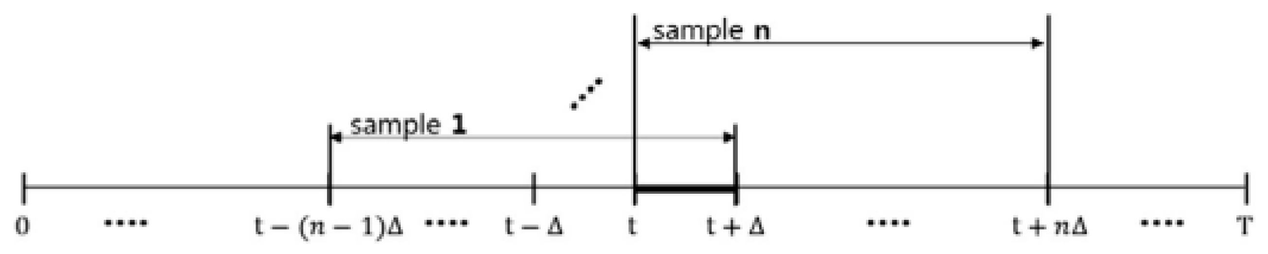
The MRDM procedure is as follows. Let us consider a sample window with fixed width , which is rolled forward by △ units each time. In each window, the aforementioned multifractality test is performed, and the result of the test (1 if the test rejects the null and 0 otherwise) is recorded. The result for window i may be denoted by , where is the indicator function. Now, consider that the period of interest is , which is included in n moving windows, as shown in Figure 1.

Figure 1.
The time range included in n sample windows. Reprinted from [13], Copyright (2015), with permission from Elsevier.
Hence, there are n windows in the period that contain . Multifractality is checked in through the proportion index:
represents the proportion of the n windows containing that reject . Following the same convention as [13], the existence of multifractality in is assumed to hold if the proportion index is above a certain threshold value, , which the authors propose to be 0.7.
4. Data and Preliminary Analysis
The database, retrieved from the Bitcoincharts API website (http://api.bitcoincharts.com/v1/csv/ (accessed on 28 July 2020)), contains the trading information on bitcoin from one of the main bitcoin online exchanges—Bitstamp. The data file contains the timestamp in Unix time, the trading price in USD, and the trading volume in bitcoin units. A significant part of these volumes is not integers, because bitcoin may be traded in multiples of of a bitcoin, i.e., a satoshi. These raw data were then sampled considering the last price before each minute observation point. The final data are formed by 3,981,601 1 min observations covering the period from 1 January 2013 to 26 July 2020.
The time series of bitcoin prices were then used to compute the logarithmic returns, such that , where is the transaction price at minute t, and is the transaction price in the previous minute. Figure 2 plots the series of 1 min bitcoin prices and the resulting logarithmic returns, with Unix time converted into calendar time.
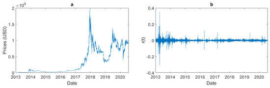
Figure 2.
One minute bitcoin prices (a) and one minute bitcoin returns (b).
Figure 2 shows that bitcoin prices have increased their scale considerably. In 2013, prices were relatively low and seemed stable. However, the history of 1 min returns in Figure 2b shows that returns are more volatile at the beginning of the sample; hence, the stability of prices in that period is merely illusory due to shifts in the price scale during the overall sample. At the end of 2013, the market experienced its first period of exponential price increase, i.e., the first considerable bubble-like event. During the following three years, prices remained at similar levels. However, in 2017 there was the second and most important bubble (in our sample). At the beginning of 2017, bitcoin was quoted at around USD 1000, and at the end of that year, it achieved the absolute maximum in this sample of almost USD 20,000. In 2018, the bubble burst, and prices showed a sharp decline. In November 2018, one may even observe a “negative” jump halving the price from USD 6000 to USD 3000. In the first semester of 2019, there was the third long-duration bubble, while in the second semester there was a reverse tendency. Finally, in February/March 2020, there was a sharp decrease, which was associated with the impact of the COVID-19 pandemic crisis. Our sample ends in July 2020, when bitcoin was quoted around USD 10,000. Arguably, the 2013 and 2017 peaks came from boosts in the popularity of bitcoin [33], and the sharp decline at the beginning of 2018 was associated with the launch of bitcoin futures by the Chicago Board Options Exchange (CBOE) and the Chicago Mercantile Exchange (CME) [54].
Table 1 presents the descriptive statistics of 1 min bitcoin returns. The mean is positive but very close to zero, and there is positive skewness, which commonly indicates that the distribution has a fatter right tail, and very high kurtosis, indicating a highly leptokurtic distribution. This extremely high kurtosis, which is pervasive at various periodicities, has itself been addressed in the literature on multifractality [24,28]. The Jarque–Bera test peremptorily rejects the null hypothesis of normality. The first-order autocorrelation is significantly negative, corroborating the result present in [27] for the 1 min returns of the bitcoin price index in the period 2014–2016.

Table 1.
Descriptive statistics of 1 min bitcoin returns.
To obtain a more complete picture of what has happened with bitcoin, namely in terms of trading intensity, we also looked at the historical data of the daily volume of the overall bitcoin market. These data were collected from CoinMarketCap from 29 April 2013 to 30 July 2020 (2650 observations). This site provides aggregated data of eligible online exchanges on daily opening, lowest, highest, and closing prices (which are commonly referred to as OLHC prices); volume; and market capitalization, all in USD. The daily volume in bitcoin units is estimated by dividing the volume in USD by the average of the OLHC prices. Figure 3 plots the daily volume.
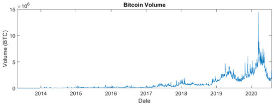
Figure 3.
Daily volume of bitcoin.
Daily trading volume had a stable increase during the years of 2013–2016, increased markedly in 2017, and then remained stable in 2018. In 2019, it increased in the first semester and decreased in part of the second semester, which was directly related to the price tendencies. Interestingly, in 2020, volume and price trends are inversely related, that is, higher volume was associated with selling pressure and decaying prices, with the peak in trading volume occurring during the COVID-19 pandemic crisis. On average, during the overall period, the eligible exchanges traded around 848 bitcoins per day, but there were some days without trading. The maximum traded volume in just one day was 14,450 bitcoins.
5. Multifractality in 1 min Bitcoin Returns
This section applies Multifractal Detrended Fluctuation Analysis (MF-DFA) to bitcoin 1 min logarithmic returns, using the code provided by [51], and uses a Multifractal Regime Detecting Method (MRDM), based on the MF-DFA Hurst exponents, to identify the time ranges when multifractality is almost surely present.
To apply MF-DFA, we use the following parameters: (1) the scaling parameter ranges from to in powers of two, (2) q ranges from −5 to 5 with a step of 0.1, and (3) the polynomial order is . According to [51], one should choose , where N is the length of the time series. Here, the minimum and maximum scales were chosen to be powers of two between those boundaries.
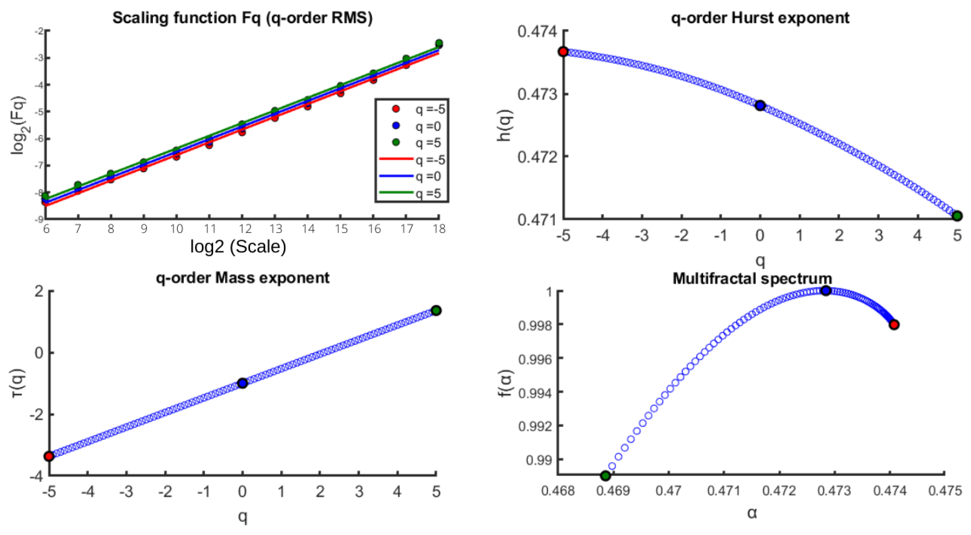
Figure 4 presents the plot of on for 101 different q orders and the plot of on for the values , , and .
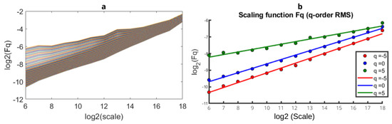
Figure 4.
(a) Plot of on for 101 different q orders and (b) plot of on for three q orders.
Figure 4 shows that the estimate of the generalized Hurst exponent, , changes for different orders q, and there is a significant difference in the fluctuation function for different orders in smaller size segments (left side of each plot).
Figure 5 shows the plot of and on q.
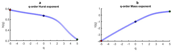
Figure 5.
(a) Plot of on q and (b) plot of on q.
Figure 5a shows that decreases non-linearly with respect to q. Most fluctuations are persistent , but this behaviour is more evident in small fluctuations, i.e., for . For , the fluctuations are anti-persistent. Therefore, for small fluctuations, the bitcoin market presents long memory. According to Figure 5b, the Rényi exponent presents a non-linear behaviour on q (because , and is not constant) and the steepest slope for values of q up to . Finally, the multifractal spectrum , shown in Figure 6, presents a single-humped shape. These figures provide clear evidence that 1 min bitcoin returns are multifractal.

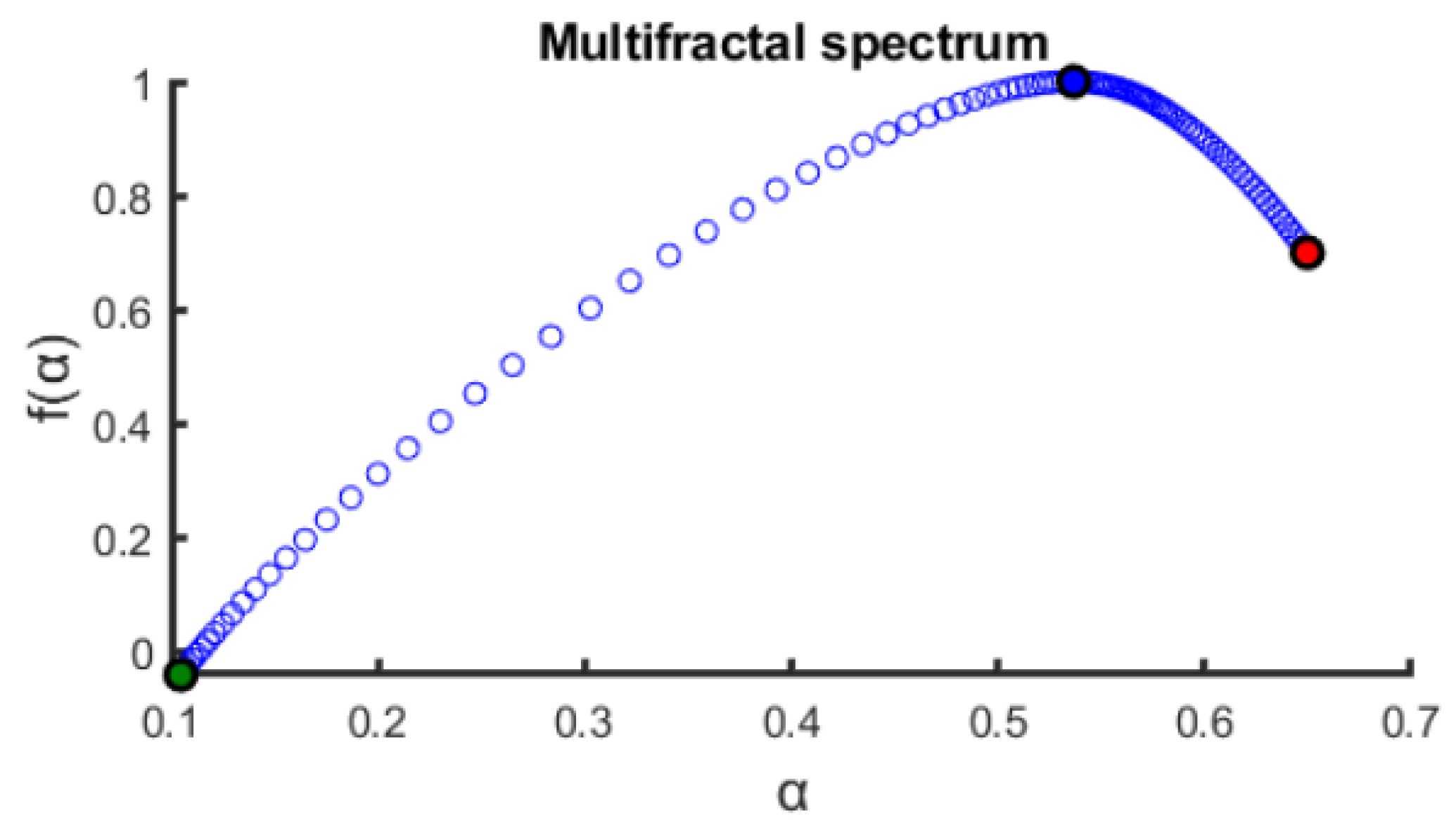
Figure 6.
The multifractal spectrum versus .
Several insights can be obtained from the multifractal spectrum (Figure 6). First, the degree of multifractality measured by Equation (3) is . This is lower than the value obtained by [27] using 1 min data from 1 January 2014 to 31 December 2016. Second, the width of the spectrum given by Equation (8) is . Third, one of the important values in the spectrum is , which gives the maximum of , i.e., , and hence measures persistence in the time series [32]. In this case, , which is a value relatively close to 0.5. Fourth, the asymmetry parameter, given by Equation (9), is , indicating that the spectrum is left-skewed, and hence large fluctuations dominate the multifractal behaviour.
For these time series, (see Equation (4)), which is a value usually interpreted as sufficiently different from zero, hence indicating informational inefficiency.
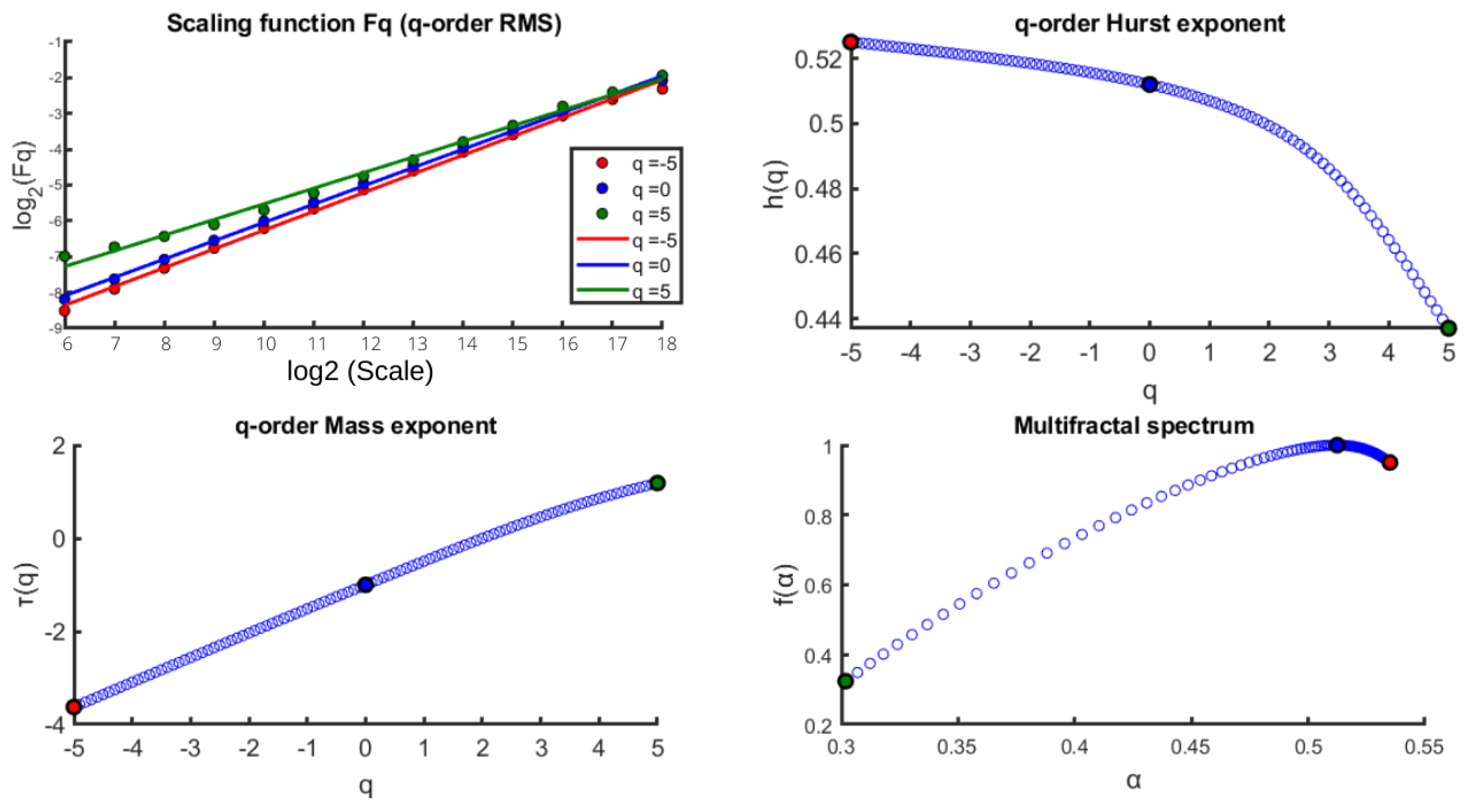
We proceed by studying the sources of multifractality. Figure 7 shows the results of MF-DFA applied to the shuffled series. The lines vs. are not parallel for different q orders, although for and the slopes are similar. In the graph of on q, there is a higher variation of for , while for , is approximately constant. Only for a few orders of q does present a value lower than 0.5. Additionally, the Rényi exponent presents lower non-linearity compared to the original series. These results suggest that the multifractality comes from the long-range correlations but also from fat-tails, since there is still evidence of multifractality in the shuffled series.
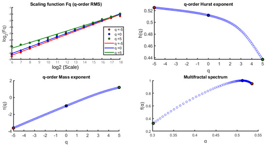
Figure 7.
MF-DFA for the shuffled series of the 1 min bitcoin returns.
Table 2 compares the degree of multifractality, ; the width of the spectrum, ; and the asymmetry parameter, A, of the original and shuffled series. All these values are lower for the transformed series, indicating that multifractality is weaker in the shuffled series, and thus long-range correlations are also a source of multifractality. This result is in accordance with [27,28,32,42].
Table 2.
Original series vs. shuffled series: Degree of multifractality, width of multifractal spectrum, and asymmetry parameter.
To obtain the surrogate series, we apply the Fourier transform (FT), which is the basis of phase randomization. We use the method of [55,56]. Here, we used a MATLAB code provided by [57]. Figure 8 shows the results of the MF-DFA for the surrogate series.
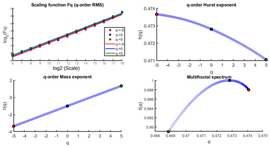
Figure 8.
MF-DFA for the surrogate series of bitcoin 1 min returns.
The slopes of for different orders are apparently parallel, which indicates that the surrogate series are almost monofractal for the domain of q used. There is a small variation of , since for , varies approximately around 0.47. The Rényi exponent is almost linear. The existing multifractality in the surrogate series is therefore very weak; hence, the importance of long-range correlations is rather low when compared with the importance of fat-tails as a source of multifractality.
Table 3 presents a similar comparison as in Table 2, but now for the surrogate series. The degree of multifractality, , and the width of the multifractal spectrum, , are very small. The weak multifractality remaining in the surrogate series is due to the long-range correlations.
Table 3.
Original series vs. surrogate series: degree of multifractality, width of multifractal spectrum, and asymmetry parameter.
In sum, both sources of multifractality are present in the 1 min returns, but clearly fat-tails are the most important. This is in accordance with the literature. For instance, [27,28,32,42], conclude that both sources of multifractality are present in the bitcoin returns, while [26,30] go further by indicating that the fat-tails are the main source of multifractality.
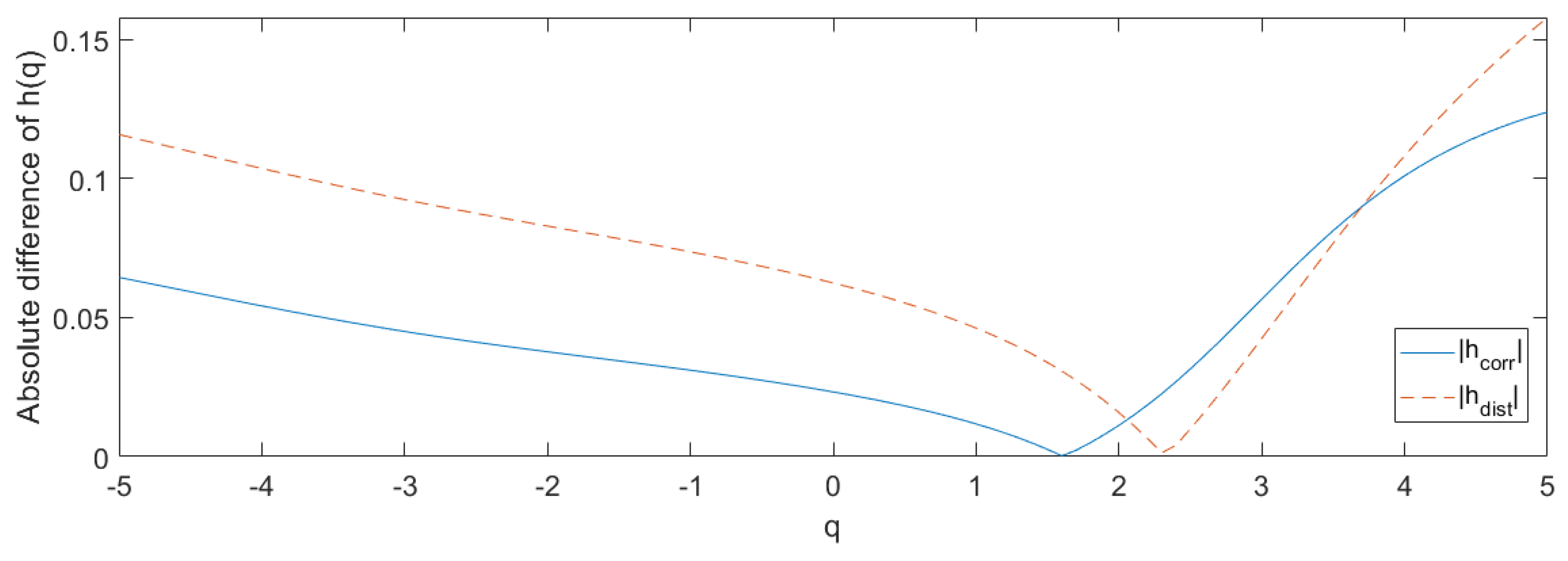
The application of the procedure proposed by [52] (see Equations (10) and (11)) is illustrated in Figure 9.
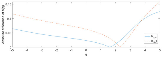
Figure 9.
Absolute differences between the generalized Hurst exponents of original and shuffled series, , and between the generalized Hurst exponents of original and surrogate series, , as a function of q.
Non-zero values of and prove that both sources of multifractality are present; however, for almost all values of q, is greater than , corroborating the previous claim that the multifractality comes mainly from fat-tails.
Before applying our multifractality test, we check its sensitiveness to and q. We apply the test to the overall sample considering and and and . We also consider and use two different subsets for , namely , and with . The results are presented in Table 4. For and , the test rejects the null hypothesis at a significance level of 0.05 only for higher scales, implying that smaller cycles are better characterized by monofractality. For and , the test suggests multifractality for all the maximum time scales considered. Thus, the farther apart the values of q are, the bigger the differences between the vectors will be, and hence more compelling evidence on multifractality is drawn from the test.
Table 4.
Multifractality Wilcoxon rank-sum test for the full sample.
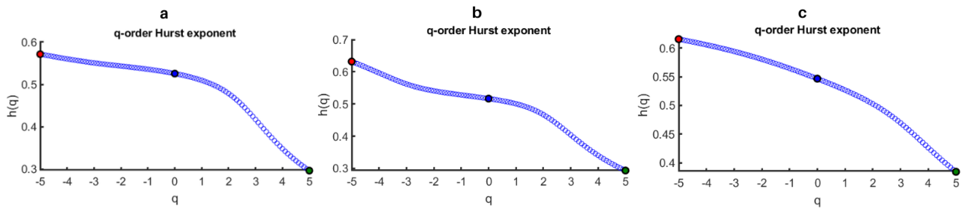
The year of 2017 is a turning point in the bitcoin market in terms of price appreciation and trading volume (see Figure 2 and Figure 3). In order to check if the fractal behaviour of bitcoin is similar before and after 2017, we partitioned the 1 min return series into two sub-samples, 16 July 2017 being the splitting day (the same one used in [33]). Figure 10 presents the generalized Hurst exponents for the two sub-samples and for the full sample for comparison purposes. These exponents were computed using the same parameters as before, except , which is now instead of , due to the smaller length of the returns series in the sub-samples.
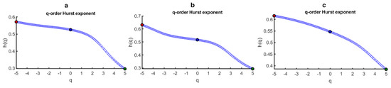
Figure 10.
Plots of on q for: (a) full sample (1 January 2013 to 26 July 2020), (b) 1st sub-sample (1 January 2013 to 16 July 2017), and (c) 2nd sub-sample (17 July 2017 to 26 July 2020).
From Figure 10, it is clear that the previous claim for the overall sample that smaller fluctuations are persistent, while larger ones are anti-persistent, is validated in the two sub-samples. The results presented in Table 5 concerning the Wilcoxon rank-sum test for the full sample and sub-samples highlight that although multifractality is most probably present in the two sub-samples, its degree and richness is higher in the second sub-sample, which is in accordance with [33].
Table 5.
Multifractality Wilcoxon rank-sum test for the full sample and sub-samples (splitting day: 16 July 2017).
Hereafter, we present the results of the MRDM. We decided to be conservative and use and . We recall that if the test fails to reject the null, this does not mean that in a given time frame the market is monofractal; it simply means that the degree of multifractality is lower. The other parameters chosen for the MRDM are the following: (1) the time range of interest is a calendar week, i.e., ; (2) the sample window is equivalent to 4 months, so , having a length of min; (3) ; (4) (notice that is the maximum power of two smaller than , where ); (5) a significance level of 5%; and (6) a threshold for .
The proportion index is computed over 365 weeks, so each value in the graph represents one week. The first week is from 15 April 2013 to 21 April 2013, leaving 15 weeks behind, in order to have the associated period . The second week goes from 22 April 2013 to 28 April 2013, and so on. The last week is from 6 April 2020 to 12 April 2020, in order to have the associated period .
Figure 11 presents the results of the MRDM.
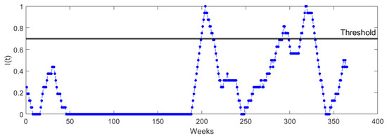
Figure 11.
MRDM applied to the 1 min bitcoin returns.
In the first half of the sample, there are several consecutive weeks where , which indicates non-multifractality, which, most probably, just implies a lower degree of multifractality. This behaviour happens from week 46 to week 188 (February 2014 to November 2016). For most of the weeks, there are always some windows where there is an indication of multifractality; however, considering the threshold of for , the existence of multifractality is only identifiable in weeks 200 to 212 (February 2017–April 2017), 292 to 298 (November 2018–December 2018), and 313 to 328 (April 2019–July 2019).
6. Conclusions
Recently, the economics and finance literature on cryptocurrencies and most notably on bitcoin has been piling up at an impressive rate, due to its impressive price appreciation, trading volume, and market capitalization. Most of this literature gathers evidence on stylized facts of bitcoin price dynamics, which appear to be different from currency exchange rates or other financial assets traded in regulated markets.
This study aims at analysing the fractality of bitcoin and hence contributes to the literature on the characterization of its price dynamics. This analysis is conducted using Multifractal Detrended Fluctuation Analysis (MF-DFA) and a Multifractal Regime Detecting Method (MRDM). The implementation of the MRDM has an originality twist because we use the estimations of the generalized Hurst exponents obtained from MF-DFA. These methodologies are applied to 1 min bitcoin returns (in USD) of Bitstamp (one of the most mature, liquid, and reputable cryptocurrency online exchanges) from January 2013 to July 2020.
Bitcoin 1 min returns are prone to extreme volatility events, present severe jumps (the minimum and maximum returns in the sample are −30.65% and 35.29%), and are highly leptokurtic. Our results indicate multifractality, with smaller fluctuations being persistent and larger ones being anti-persistent. On the one hand, multifractality comes in part from significant long-range correlations, which cast some doubts on the informational efficiency of high-frequency bitcoin prices at Bitstamp; on the other hand, multifractality mainly comes from fat-tails, which highlights the high level of short-run risk that investors face in this market.
The results also highlight that fractal dynamics are themselves time-varying. The MRDM shows that, roughly speaking, a higher degree of multifractality is most probably present in the last half of the series, more precisely in and after 2017. Our conservative approach, for scaling factors of 1 and 2, detects multifractality in the first quarter of 2017, last quarter of 2018, and second quarter of 2019, while the absence of multifractality at these scaling factors most probably characterizes the period from February 2014 to November 2016. The analogy of the “wind tunnel” [9] may shed some light on a possible explanation of these changes in the degree of multifractality. The complex behaviour of the wind inside a tunnel arises when the wind speed (i.e., the tunnel pressure) increases or when the tunnel opening narrows. Therefore, one may argue that the complexity of bitcoin is caused by the pressure of increasing demand (that is, an increase in the “tunnel pressure”) or by a more inelastic supply (that is, a “narrow tunnel opening”).
Noticeably, the timing of major upward shifts in bitcoin prices coincides with the “recovery” of long-run interest rates, which may induce agents (including the most speculative ones) to believe that in the near future, there will be a sustained increase in the supply of fiat currencies. Arguably, at those periods there is a boost in the attractiveness of bitcoin due to its relatively inelastic supply. Hence, the inelasticity of bitcoin supply is an incentive to increase its demand, especially if there are expectations that the central banks intend to undergo a more expansionary monetary policy.
In sum, the long-run attractiveness and increasing valuation of bitcoin and its corresponding short-run instability are intertwined features that go together as if they were “two faces of the same coin”.
Author Contributions
Conceptualization, C.V., R.P. and H.S.; Data curation, C.V. and H.S.; Formal analysis, R.P.; Investigation, C.V.; Methodology, C.V., R.P. and H.S.; Supervision, R.P. and H.S.; Validation, R.P. and H.S.; Visualization, H.S.; Writing—original draft, C.V.; Writing—review and editing, R.P. and H.S. All authors have read and agreed to the published version of the manuscript.
Funding
This work has been funded by national funds through FCT—Fundação para a Ciência e a Tecnologia, I.P., Project UIDB/05037/2020.
Institutional Review Board Statement
Not applicable.
Informed Consent Statement
Not applicable.
Data Availability Statement
Data used in this study was obtained from the Bitcoincharts API website (http://api.bitcoincharts.com/v1/csv/ (accessed on 28 July 2020)).
Conflicts of Interest
The authors declare no conflict of interest.
References
- Nakamoto, S. Bitcoin: A Peer-to-Peer Electronic Cash System. 2008. Available online: https://bitcoin.org/bitcoin.pdf (accessed on 18 September 2020).
- Bariviera, A.F.; Basgall, M.J.; Hasperué, W.; Naiouf, M. Some stylized facts of the Bitcoin market. Phys. A Stat. Mech. Its Appl. 2017, 484, 82–90. [Google Scholar] [CrossRef] [Green Version]
- Sebastião, H.; Godinho, P. Forecasting and trading cryptocurrencies with machine learning under changing market conditions. Financ. Innov. 2021, 7, 1–30. [Google Scholar] [CrossRef]
- Gunay, S. Source of the multifractality in exchange markets: Multifractal detrended fluctuations analysis. J. Bus. Econ. Res. (JBER) 2014, 12, 371–384. [Google Scholar] [CrossRef] [Green Version]
- Fama, E.F. Efficient capital markets: A review of theory and empirical work. J. Financ. 1970, 25, 383–417. [Google Scholar] [CrossRef]
- Peters, E.E. Fractal Market Analysis: Applying Chaos Theory to Investment and Economics; John Wiley & Sons: Hoboken, NJ, USA, 1994; Volume 24. [Google Scholar]
- Kristoufek, L. Fractal markets hypothesis and the global financial crisis: Scaling, investment horizons and liquidity. Adv. Complex Syst. 2012, 15, 1250065. [Google Scholar] [CrossRef] [Green Version]
- Anderson, N.; Noss, J. The Fractal Market Hypothesis and Its Implications for the Stability of Financial Markets. Bank of England Financial Stability Paper. 2013, Volume 23. Available online: https://ssrn.com/abstract=2338439 (accessed on 18 September 2020).
- Mandelbrot, B.B.; Hudson, R.L. The (Mis) Behaviour of Markets: A Fractal View of Risk, Ruin and Reward; Profile Books: London, UK, 2010. [Google Scholar]
- Mandelbrot, B.B.; Fisher, A.J.; Calvet, L.E. A Multifractal Model of Asset Returns. Cowles Foundation Discussion Paper. 1997, Volume 1164. Available online: https://ssrn.com/abstract=78588 (accessed on 18 September 2020).
- Kantelhardt, J.W.; Zschiegner, S.A.; Koscielny-Bunde, E.; Havlin, S.; Bunde, A.; Stanley, H.E. Multifractal detrended fluctuation analysis of nonstationary time series. Phys. A Stat. Mech. Its Appl. 2002, 316, 87–114. [Google Scholar] [CrossRef] [Green Version]
- Peng, C.K.; Buldyrev, S.V.; Havlin, S.; Simons, M.; Stanley, H.E.; Goldberger, A.L. Mosaic organization of DNA nucleotides. Phys. Rev. E 1994, 49, 1685. [Google Scholar] [CrossRef] [Green Version]
- Lee, H.; Chang, W. Multifractal regime detecting method for financial time series. Chaos Solitons Fractals 2015, 70, 117–129. [Google Scholar] [CrossRef]
- Mandelbrot, B. Statistical methodology for nonperiodic cycles: From the covariance to R/S analysis. In Annals of Economic and Social Measurement; NBER: Berlin, Germany, 1972; Volume 1, pp. 259–290. [Google Scholar]
- Suárez-García, P.; Gómez-Ullate, D. Multifractality and long memory of a financial index. Phys. A Stat. Mech. Its Appl. 2014, 394, 226–234. [Google Scholar] [CrossRef] [Green Version]
- Wang, Y.; Wei, Y.; Wu, C. Analysis of the efficiency and multifractality of gold markets based on multifractal detrended fluctuation analysis. Phys. A Stat. Mech. Its Appl. 2011, 390, 817–827. [Google Scholar] [CrossRef]
- Lim, G.; Kim, S.; Lee, H.; Kim, K.; Lee, D.I. Multifractal detrended fluctuation analysis of derivative and spot markets. Phys. A Stat. Mech. Its Appl. 2007, 386, 259–266. [Google Scholar] [CrossRef]
- Fernandes, L.H.S.; Araújo, F.H.A.; Silva, I.E.M.; Leite, U.P.S.; de Lima, N.F.; Stosic, T.; Ferreira, T.A.E. Multifractal behavior in the dynamics of Brazilian inflation indices. Phys. A Stat. Mech. Its Appl. 2020, 2020, 124158. [Google Scholar] [CrossRef]
- Urquhart, A. The inefficiency of Bitcoin. Econ. Lett. 2016, 148, 80–82. [Google Scholar] [CrossRef]
- Kristoufek, L.; Vosvrda, M. Measuring capital market efficiency: Global and local correlations structure. Phys. A Stat. Mech. Its Appl. 2013, 392, 184–193. [Google Scholar] [CrossRef] [Green Version]
- Kristoufek, L.; Vosvrda, M. Gold, currencies and market efficiency. Phys. A Stat. Mech. Its Appl. 2016, 449, 27–34. [Google Scholar] [CrossRef] [Green Version]
- Kristoufek, L. On Bitcoin markets (in) efficiency and its evolution. Phys. A Stat. Mech. Its Appl. 2018, 503, 257–262. [Google Scholar] [CrossRef]
- Fang, W.; Tian, S.; Wang, J. Multiscale fluctuations and complexity synchronization of Bitcoin in China and US markets. Phys. A Stat. Mech. Its Appl. 2018, 512, 109–120. [Google Scholar] [CrossRef]
- Bariviera, A.F. The inefficiency of Bitcoin revisited: A dynamic approach. Econ. Lett. 2017, 161, 1–4. [Google Scholar] [CrossRef] [Green Version]
- Jiang, Y.; Nie, H.; Ruan, W. Time-varying long-term memory in Bitcoin market. Financ. Res. Lett. 2018, 25, 280–284. [Google Scholar] [CrossRef]
- Lahmiri, S.; Bekiros, S. Chaos, randomness and multi-fractality in Bitcoin market. Chaos Solitons Fractals 2018, 106, 28–34. [Google Scholar] [CrossRef]
- Takaishi, T. Statistical properties and multifractality of Bitcoin. Phys. A Stat. Mech. Its Appl. 2018, 506, 507–519. [Google Scholar] [CrossRef] [Green Version]
- Filho, A.C.d.S.; Maganini, N.D.; de Almeida, E.F. Multifractal analysis of Bitcoin market. Phys. A Stat. Mech. Its Appl. 2018, 512, 954–967. [Google Scholar] [CrossRef]
- Al-Yahyaee, K.H.; Mensi, W.; Yoon, S.M. Efficiency, multifractality, and the long-memory property of the Bitcoin market: A comparative analysis with stock, currency, and gold markets. Financ. Res. Lett. 2018, 27, 228–234. [Google Scholar] [CrossRef]
- Zhang, X.; Yang, L.; Zhu, Y. Analysis of multifractal characterization of Bitcoin market based on multifractal detrended fluctuation analysis. Phys. A Stat. Mech. Its Appl. 2019, 523, 973–983. [Google Scholar] [CrossRef]
- Stavroyiannis, S.; Babalos, V.; Bekiros, S.; Lahmiri, S.; Uddin, G.S. The high frequency multifractal properties of Bitcoin. Phys. A Stat. Mech. Its Appl. 2019, 520, 62–71. [Google Scholar] [CrossRef]
- Telli, Ş.; Chen, H. Multifractal behavior in return and volatility series of Bitcoin and gold in comparison. Chaos Solitons Fractals 2020, 139, 109994. [Google Scholar] [CrossRef]
- Jiang, C.; Dev, P.; Maller, R.A. A Hypothesis Test Method for Detecting Multifractal Scaling, Applied to Bitcoin Prices. J. Risk Financ. Manag. 2020, 13, 104. [Google Scholar] [CrossRef]
- Tiwari, A.K.; Jana, R.K.; Das, D.; Roubaud, D. Informational efficiency of Bitcoin—An extension. Econ. Lett. 2018, 163, 106–109. [Google Scholar] [CrossRef]
- Garnier, J.; Solna, K. Chaos and order in the bitcoin market. Phys. A Stat. Mech. Its Appl. 2019, 524, 708–721. [Google Scholar] [CrossRef] [Green Version]
- Caporale, G.M.; Gil-Alana, L.; Plastun, A. Persistence in the cryptocurrency market. Res. Int. Bus. Financ. 2018, 46, 141–148. [Google Scholar] [CrossRef]
- Zhang, W.; Wang, P.; Li, X.; Shen, D. The inefficiency of cryptocurrency and its cross-correlation with Dow Jones Industrial Average. Phys. A Stat. Mech. Its Appl. 2018, 510, 658–670. [Google Scholar] [CrossRef]
- Mensi, W.; Lee, Y.J.; Al-Yahyaee, K.H.; Sensoy, A.; Yoon, S.M. Intraday downward/upward multifractality and long memory in Bitcoin and Ethereum markets: An asymmetric multifractal detrended fluctuation analysis. Financ. Res. Lett. 2019, 31, 19–25. [Google Scholar] [CrossRef]
- Costa, N.; Silva, C.; Ferreira, P. Long-range behaviour and correlation in DFA and DCCA analysis of cryptocurrencies. Int. J. Financ. Stud. 2019, 7, 51. [Google Scholar] [CrossRef] [Green Version]
- Derbentsev, V.; Kibalnyk, L.; Radzihovska, Y. Modelling multifractal properties of cryptocurrency market. Period. Eng. Nat. Sci. 2019, 7, 690–701. [Google Scholar] [CrossRef]
- Cheng, Q.; Liu, X.; Zhu, X. Cryptocurrency momentum effect: DFA and MF-DFA analysis. Phys. A Stat. Mech. Its Appl. 2019, 526, 120847. [Google Scholar] [CrossRef]
- Stosic, D.; Stosic, D.; Ludermir, T.B.; Stosic, T. Multifractal behavior of price and volume changes in the cryptocurrency market. Phys. A Stat. Mech. Its Appl. 2019, 520, 54–61. [Google Scholar] [CrossRef]
- Kristjanpoller, W.; Bouri, E. Asymmetric multifractal cross-correlations between the main world currencies and the main cryptocurrencies. Phys. A Stat. Mech. Its Appl. 2019, 523, 1057–1071. [Google Scholar] [CrossRef]
- Bariviera, A.F. One model is not enough: Heterogeneity in cryptocurrencies’ multifractal profiles. Financ. Res. Lett. 2021, 39, 101649. [Google Scholar] [CrossRef]
- Mnif, E.; Jarboui, A.; Mouakhar, K. How the cryptocurrency market has performed during COVID 19? A multifractal analysis. Financ. Res. Lett. 2020, 36, 101647. [Google Scholar] [CrossRef] [PubMed]
- Zhang, Y.; Chan, S.; Chu, J.; Nadarajah, S. Stylised facts for high frequency cryptocurrency data. Phys. A Stat. Mech. Its Appl. 2019, 513, 598–612. [Google Scholar] [CrossRef]
- Naeem, M.A.; Bouri, E.; Peng, Z.; Shahzad, S.J.H.; Vo, X.V. Asymmetric efficiency of cryptocurrencies during COVID19. Phys. A Stat. Mech. Its Appl. 2021, 565, 125562. [Google Scholar] [CrossRef]
- Kantelhardt, J.W. Fractal and multifractal time series. arXiv 2008, arXiv:0804.0747. [Google Scholar]
- Wang, Y.; Liu, L.; Gu, R. Analysis of efficiency for Shenzhen stock market based on multifractal detrended fluctuation analysis. Int. Rev. Financ. Anal. 2009, 18, 271–276. [Google Scholar] [CrossRef]
- Calvet, L.E.; Fisher, A.J.; Mandelbrot, B.B. Large Deviations and the Distribution of Price Changes. Cowles Foundation Discussion Paper. 1997, Volume 1165. Available online: https://ssrn.com/abstract=78608 (accessed on 18 September 2020).
- Ihlen, E.A.F.E. Introduction to multifractal detrended fluctuation analysis in Matlab. Front. Physiol. 2012, 3, 141. [Google Scholar] [CrossRef] [PubMed] [Green Version]
- Baranowski, P.; Krzyszczak, J.; Slawinski, C.; Hoffmann, H.; Kozyra, J.; Nieróbca, A.; Siwek, K.; Gluza, A. Multifractal analysis of meteorological time series to assess climate impacts. Clim. Res. 2015, 65, 39–52. [Google Scholar] [CrossRef] [Green Version]
- Di Matteo, T.; Aste, T.; Dacorogna, M.M. Scaling behaviors in differently developed markets. Phys. A Stat. Mech. Its Appl. 2003, 324, 183–188. [Google Scholar] [CrossRef]
- Sebastião, H.; Godinho, P. Bitcoin Futures: An Effective Tool for Hedging Cryptocurrencies. Financ. Res. Lett. 2020, 33, 101230. [Google Scholar] [CrossRef]
- Theiler, J.; Eubank, S.; Longtin, A.; Galdrikian, B.; Farmer, J.D. Testing for nonlinearity in time series: The method of surrogate data. Phys. D Nonlinear Phenom. 1992, 58, 77–94. [Google Scholar] [CrossRef] [Green Version]
- Schreiber, T.; Schmitz, A. Surrogate time series. Phys. D Nonlinear Phenom. 2000, 142, 346–382. [Google Scholar] [CrossRef] [Green Version]
- Temu. Surrogate Data. MATLAB Central File Exchange. 2020. Available online: https://www.mathworks.com/matlabcentral/fileexchange/4612-surrogate-data (accessed on 15 December 2020).


Publisher’s Note: MDPI stays neutral with regard to jurisdictional claims in published maps and institutional affiliations. |
© 2021 by the authors. Licensee MDPI, Basel, Switzerland. This article is an open access article distributed under the terms and conditions of the Creative Commons Attribution (CC BY) license (https://creativecommons.org/licenses/by/4.0/).