Abstract
In this artificial intelligence era, the constantly changing technology makes production techniques become sophisticated and complicated. Therefore, manufacturers are dedicated to improving the quality of products by increasing the lifetime in order to achieve the quality standards demanded by consumers. For products with lifetime following a Gompertz distribution, the lifetime performance index was used to measure the performance of manufacturing process under progressive type I interval censoring. The sampling design is investigated to reach the given level of significance and power level. When inspection interval length is fixed and the number of inspection intervals is not fixed, the required number of inspection intervals and sample size with minimum total cost are determined and tabulated. When the termination time is not fixed, the required number of inspection intervals, sample size, and equal interval length reaching the minimum total cost are determined and tabulated. The optimal parameter values are tabulated for the practical use of users. Finally, one practical example is given for the illustrative aim to show the implementation of this sampling design to collect data and the collected data are used to conduct the testing procedure to see if the process is capable.
1. Introduction
Montgomery [1] presented the lifetime performance index CL to measure the larger-the-better type quality characteristics—for example, lifetime, heat resistance, mpg for vehicles, etc. When the lifetime of products follows an exponential distribution, Tong et al. [2] used the uniformly minimum variance unbiased estimator (UMVUE) of CL to construct a hypothesis testing procedure for the complete sample. However, there are many cases where the experimenters can not observe the lifetimes of all the items due to the budget restrictions or time limitation, etc. The censoring is thus arisen. For progressive censoried data (see Balakrishnan and Aggarwala [3], Aggarwala [4]), Lee et al. [5] proposed a testing procedure for this lifetime performance index under progressive type II censoring. For step-stress accelerated life-testing data (see Wu et al. [6], Wu et al. [7]), Lee et al. [8] evaluated the lifetime performance index of exponential products. Wu and Lin [9] proposed a testing procedure for the lifetime performance index CL for exponential products using the maximum likelihood estimator under progressive type I interval censoring. Wu and Hsieh [10] proposed a testing procedure for Gompertz products using this index under progressive type I interval censoring and the related testing procedure is summarized in Section 2. In Section 3, we propose a sampling design to determine the minimum sample size required to attain the pre-specified power level and level of significance. Under a specific cost structure, the total cost of the experiment is considered to be minimized. When the termination time of the experiment is fixed or not fixed, the sampling design is determined separately to minimize the total cost in Section 3. The algorithms, figures, and tables are shown in this section. Our algorithms can help experimenters to setup the progressive type-I interval censoring scheme and then the experimenters can collect the progressive type-I interval censored sample under different considerations. We give an example to implement our proposed sampling design to collect the progressive type-I interval censored sample and utilize this sample to conduct the hypothesis test for the lifetime performance index CL to see if the process is capable. Finally, the conclusions are made in Section 4.
2. The Introduction of the Testing Procedure for the Lifetime Performance Index
Suppose that the lifetime U of products follows a two-parameter Gompertz distribution with the probability density function (pdf) and the cumulative distribution function (cdf) as follows:
In addition,
The Gompertz distribution is usually used to describe the human mortality. It can also model the lifetime with increasing failure rate exponentially over time.
Considering the transformation , the new lifetime variable Y has an exponential distribution with scale parameter 1/ and the pdf and cdf are given by
In addition,
Montgomery [1] presented the lifetime performance index as
where is the process mean and is the process standard deviation, and L is the known lower specification limit. Supposing that the lower specification limit for U is LU, then the lower specification limit for Y turns out to be .
The mean and the standard deviation of Y are = 1/ and = 1/. Substitute and into Equation (5); then, we have the lifetime performance index .
The conforming rate is obtained as
Apparently, the conforming rate is an increasing function of CL.
The progressive type I interval censoring scheme is addressed as follows: We put products on a life test at time 0. Determine the inspection times (t1, …, tm) and the removal percentages of the remaining survival units at time (t1, …, tm) as (p1, …, pm). The termination time for the experiment is tm = T with pm = 1. At the ith inspection time interval (ti−1, ti], the number of failure units Xi is observed and then units are randomly removed from the remaining survival units, where [w] denotes the largest integer which is smaller than or equal to w, I = 1, …, m. Then, the observed number of failure units (X1, …, Xm) is regarded as the progressive type I interval censored sample under censoring scheme (R1, …, Rm) with removal percentages (p1, …, pm). Wu and Hsieh [10] obtained the maximum likelihood estimator (MLE) of denoted by as the numerical solution of the following log-likelihood equation:
Its asymptotic variance is the reciprocal of the Fisher’s information
Then, we have
For equal interval lengths, ti − ti−1 = t and ti = it, I = 1, …, m are replaced in Equations (6) and (7).
By the property of the invariance of MLE, the MLE of can be obtained as
Suppose that c0 is the desired level of lifetime performance index to make the process capable. Then, we want to test (the process is not capable) vs. (the process is capable). Making use of the MLE of as the test statistic under the level of significance , the decision rule is to reject the null hypothesis if , where the critical value is , , and represents the percentile of the standard normal distribution.
The test power h(c1) of this statistical hypothesis test at the point of is
where is the cdf for the standard normal distribution, and .
3. Reliability Sampling Design
The reliability sampling design is very important for experimeters to plan the progressive type I interval censoring experiment. In Section 3.1, the required minimum sample size is determined under the control of the type II error (producers’ risk). In Section 3.2, under the fixed total experimental time T, the required sample size and minimal number of inspection intervals are determined to reach the given power of the level test for the testing procedure and also to minimize the total cost of experiment. In Section 3.3, for unfixed experimental termination time T, we determine the required sample size, minimal number of inspection intervals, and the equal length of interval so that the total experimental cost is minimized.
3.1. The Determination of Sample Size for Fixed m and T
In this section, the minimum sample size n is determined to reach the type II error at under significance level . Let
which is independent of the sample size n.
Set the power to be 1 − as
Solving the above equation, the minimum required sample size is obtained as
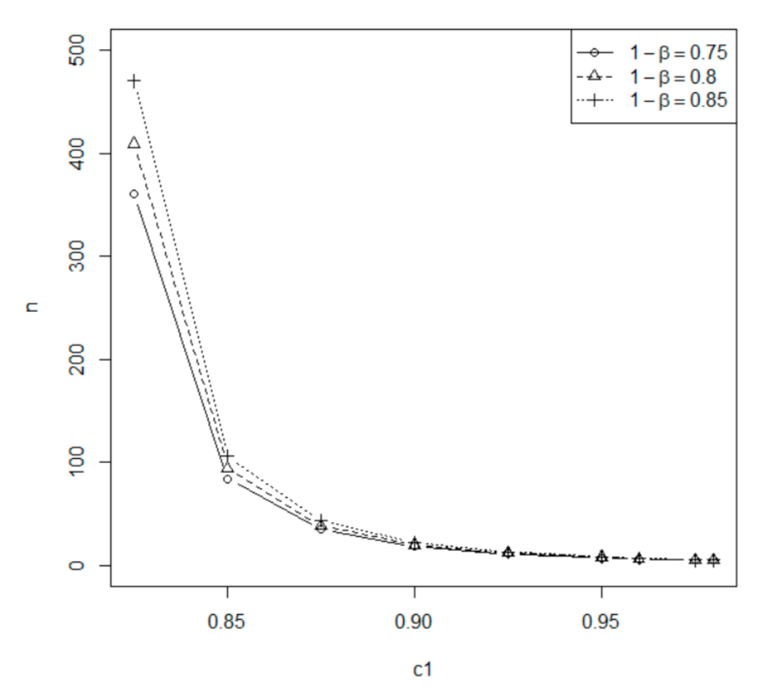
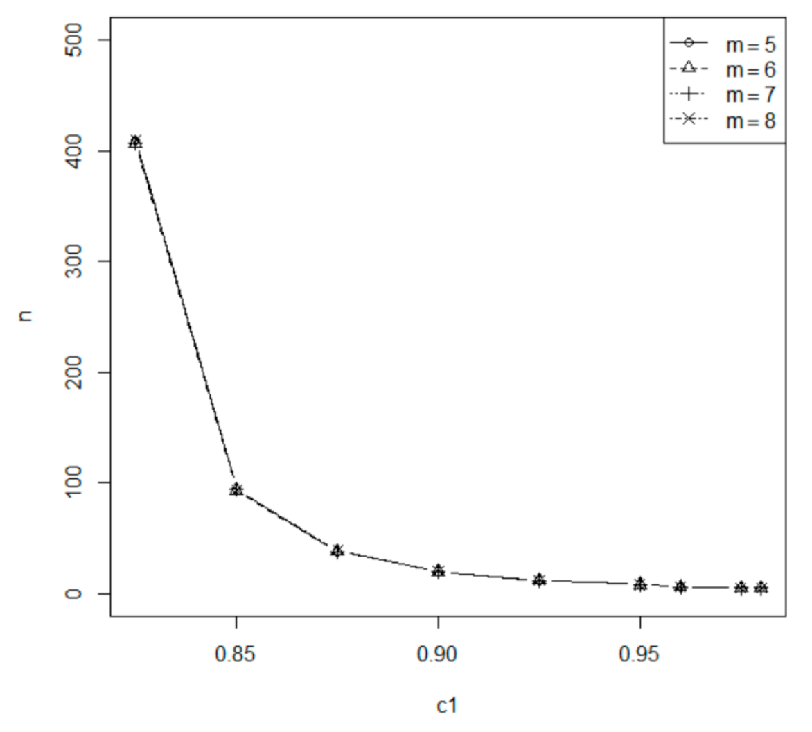
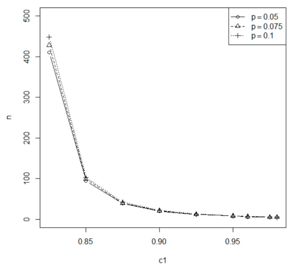
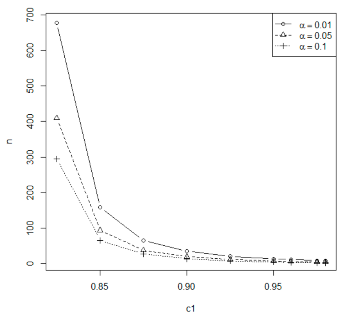
Under = 0.01, 0.05, 0.1, = 0.25, 0.20, 0.15, L = 0.05 and T = 0.5, the minimum required sample size is tabulated in Table 1, Table 2, Table 3 for c1 = 0.825(0.025)0.9, m = 5(1)8 and p = 0.05(0.025)0.1 for testing . The minimum required sample sizes are also displayed in Figure 1, Figure 2, Figure 3, Figure 4 for some typical cases. From Figure 1, Figure 2, Figure 3, Figure 4, we find that (1) the minimum required sample size decreases when increases for any combinations of , , m, and p overall speaking. (2) The minimum required sample size is a non-increasing function of probability of type II error or a non-decreasing function of power 1- at = 0.05 for fixed m = 5 and p = 0.05. (Other combinations of , m, and p also have the same pattern); (3) the change in m does not show any trend on the minimum required sample size at = 0.05 for fixed = 0.2 and p = 0.05. (Other combinations of , , and p also have the same pattern); (4) the minimum required sample size is a non-decreasing function of the removal percentage p for fixed , , and m, but the difference is not significant; (5) the minimum required sample size increases when the level of significance decreases for any combinations of , m, and p. For example, the user wants to conduct the level 0.05 hypothesis testing of under power of 0.8 at c1 = 0.95, p = 0.05, L = 0.05, T = 0.5, and m = 5 with k = 4.47, and the minimum required sample size is 8 with critical value 0.9234 from Table 2.

Table 1.
The minimum sample size for c1 = 0.825(0.025)0.9, m = 5(1)8 and p = 0.05(0.025)0.1 under = 0.01, L = 0.05, T = 0.5, and c0 = 0.8.
Table 2.
The minimum sample size for c1 = 0.825(0.025)0.9, m = 5(1)8 and p = 0.05(0.025)0.1 under = 0.05, L = 0.05, T = 0.5, and c0 = 0.8.
Table 3.
The minimum sample size for c1 = 0.825(0.025)0.9, m = 5(1)8 and p = 0.05(0.025)0.1 under = 0.01, L = 0.10, T = 0.5, and c0 = 0.8.
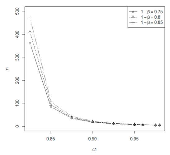
Figure 1.
Minimum sample size for the test at = 0.05, p = 0.05, and m = 5.
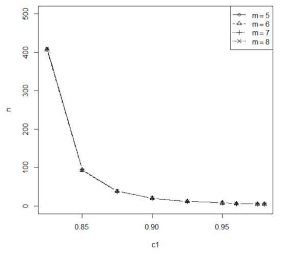
Figure 2.
Minimum sample size for the test at = 0.05, = 0.2, and p = 0.05.
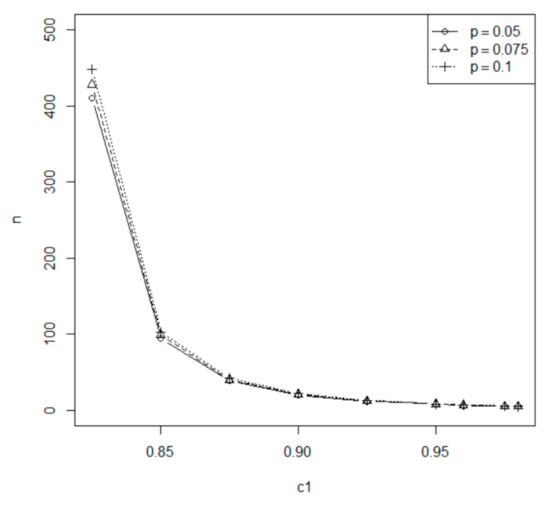
Figure 3.
Minimum sample size for the test at = 0.05, = 0.2, and m = 5.
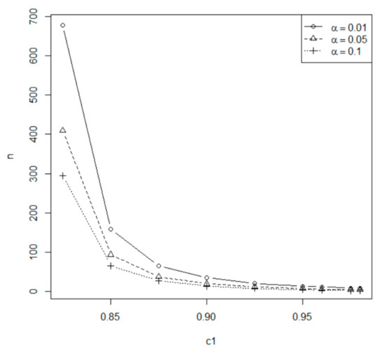
Figure 4.
Minimum sample size for the test at = 0.2 under p = 0.05 and m = 5.
3.2. The Optimal m and n for Fixed T
The experimenters usually do not prefer a large number of inspection intervals m. Not like Section 3.1, the number of inspection intervals m is needed to be determined in this section. Let m0 be the upper limit of m specified by the experimenters such that m0. (m0 is defaulted to be 100). The sample size n is the function of m. We would like to determine the optimal (m,n) to minimize the total cost occurred during the progressive type I interval censoring procedure. Similar to Huang and Wu [11], we consider the following costs:
- Installation cost Ca: the cost for installing all test units;
- Inspection cost CI: the cost for implementing the inspection equipment;
- Sample cost Cs: the cost for per test unit;
- Operation cost Co: the cost including the personnel cost, depreciation of test equipment, etc. It is proportional to the length of experimental time.
Considering all these costs, we have the total cost of
We use a numeration method to search the optimal (m,n), and the Algorithm 1 is given as follows:
| Algorithm 1 Searching for the optimal (m,n). |
| Step 1: Give the pre-assigned values of c0, c1, , , p, T, L, and m0 (the default value is 100) and the four costs Ca = aCo, Cs = bCo, CI = cCo, Co. |
| Step 2: Compute and . |
| Step 3: Set m = 1. |
| Step 4: Compute the sample size n as in Equation (11) and then compute the related total cost TC(m,n) as in Equation (12). |
| Step 5: If m < m0, then m = m + 1 and go to Step 4, else go to Step 6. |
| Step 6: The optimal solution of m* is the minimum m value such that TC* = TC(m,n) is reached and then the corresponding sample size n* is obtained. |
| Step 7: The critical value of is calculated. |
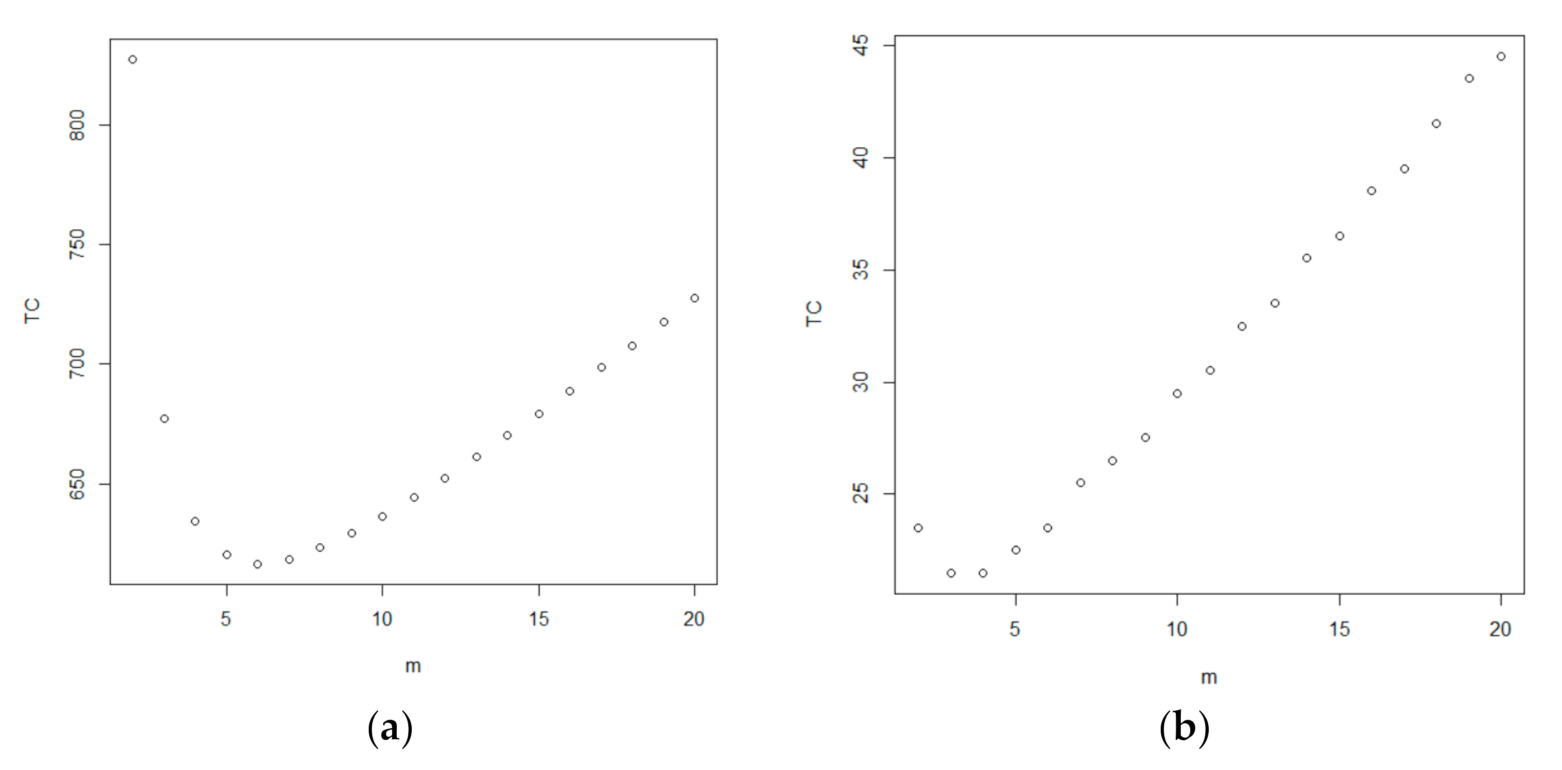
Consider Co = 1 and a = b = c = 1. For testing under = 0.01, = 0.25, p = 0.05, c1 = 0.825, k = 4.47, L = 0.05 and T = 0.5, we plot m = 2(1)m0 against its corresponding total cost in Figure 5a. You can see that minimum total cost occurred when m = 6 with the total cost of 616.5. For different set up of parameters = 0.15, = 0.1, p = 0.1, c1 = 0.9, k = 4.47, L = 0.05, T = 0.5, another total cost curve with m = 2(1)m0 is given in Figure 5b. You can see that it is a concave upward curve with some flats and the minimum total cost occurred when m = 3 with the total cost of 21.5.
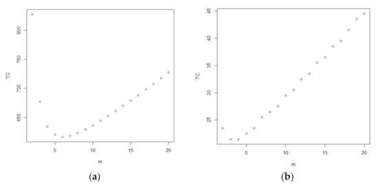
Figure 5.
(a) Total cost curve at m = 2(1) m0; (b) total cost curve at m = 2(1) m0.
The minimum suggested inspection intervals m* and sample size n* to attain minimal total cost TC(m*,n*) under the constraint of m < m0, where m0 = 20 for testing are tabulated in Table 4 and Table 5 at = 0.25, 0.20, 0.15, = 0.01, 0.05, 0.1, L = 0.05, T = 0.5, p = 0.05(0.025)0.1 for c1 = 0.825, 0.850, and c1 = 0.875, 0.90, respectively. The corresponding critical values are also tabulated.
Table 4.
The optimal (m*,n*), total cost TC and critical value for c1 = 0.825, 0.85 and p = 0.05(0.025)0.1 under m0 = 20, L = 0.05, T = 0.5, and c0 = 0.8.
Table 5.
The optimal (m*,n*), total cost TC and critical value for c1 = 0.875, 0.90 and p = 0.05(0.025)0.1 under m0 = 20, L = 0.05, T = 0.5, and c0 = 0.8.
For example, suppose that the user wants to conduct the level 0.05 hypothesis testing of under = 0.8 at c1 = 0.90, p = 0.05 and m0 = 20. From Table 5, the minimum required sample size is n* = 21 and the minimum number of inspection intervals is m* = 3. The total cost is calculated as TC = 25.5 and the critical value is 0.8799.
- (1)
- When the level of significance decreases, the minimum sample size n* is increasing for fixed and p;
- (2)
- When c1 increases, the minimum sample size n* is decreasing for fixed , , and p;
- (3)
- When the the probability of type II error decreases, the minimum sample size n* is increasing for fixed , c1, and p;
- (4)
- When c1 increases, the minimum inspection intervals m* is decreasing for fixed , , and p;
- (5)
- When decreases, the minimum inspection intervals m* is non-increasing for fixed , c1, and p;
- (6)
- When c1 increases, the minimum total cost is decreasing for fixed , , and p;
- (7)
- When decreases, the minimum total cost is increasing for fixed , c1, and p;
- (8)
- When p increases, the minimum total cost is increasing for fixed , , and c1.
3.3. The Optimal m, t, and n When the Termination Time T Is Not Fixed
We consider the case when the total life test time T is not fixed in this section. The inspection time t for each inspection interval is needed to be determined. The optimal (m,t,n) is specified to minimize the total cost occurred during the progressive type I interval censoring procedure. The total cost is
We use the numeration method to search the optimal (m,t,n) and the Algorithm 2 is given as follows:
| Algorithm 2 Searching for the optimal (m,t,n). |
| Step 1: Give the pre-assigned values of c0, c1, , and p, L and m0 (the default value is 100) and the four costs Ca = aCo, Cs = bCo, CI = cCo, Co. |
| Step 2: Compute and . |
| Step 3: Set m = 1. |
| Step 4: Find the optimal solution t* such that TC(m,t,n) is minimized. Compute the sample size n as in Equation (11) and then compute the related total cost TC(m,t*,n) as in Equation (13). |
| Step 5: If m < m0, then m = m+1 and go to Step 4, else go to Step 6. |
| Step 6: The optimal solution of m* is the minimum m value such that TC** = TC(m,t*,n) is reached and then the corresponding sample size n* is obtained. |
| Step 7: The critical value of is calculated. |
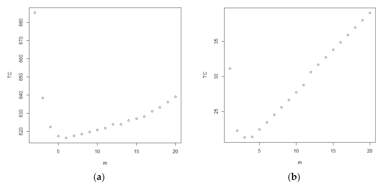
Consider Co = 1 and a = b = c = 1. For testing under = 0.25, = 0.01, p = 0.05, c1 = 0.825, k = 4.47, L = 0.05, T = 0.5, we plot m = 2(1)m0 against its corresponding total cost in Figure 6a. You can see that a minimum total cost occurred when m = 6 with the total cost of 616.476. For a different set up of parameters = 0.15, = 0.1, p = 0.1, c1 = 0.9, k = 4.47, L = 0.05, and T = 0.5, another total cost curve with m = 1(1)m0 is given in Figure 6b. You can see that it is a concave upward curve with some flats and the minimum total cost occurred when m = 3 with the total cost of 21.309. For other combination of set ups, we also find the similar patterns.

Figure 6.
(a) Total cost curve at m = 2(1)m0; (b) total cost curve at m = 1(1)m0.
The minimum suggested inspection intervals m*, inspection interval time length t* and sample size n* to yield the minimum total cost TC(m*,t*,n*) under the constraint of m< m0, where m0 = 20 for testing are tabulated in Table 6 and Table 7 at = 0.25, 0.20, 0.15, = 0.01, 0.05, 0.1, L = 0.05, p = 0.05(0.025)0.1 for c1 = 0.825, 0.850, and c1 = 0.875, 0.90, respectively. The corresponding critical values are also tabulated.
Table 6.
The optimal (m*,t*,n*), total cost TC and critical value for c1 = 0.825, 0.85 and p = 0.05(0.025)0.1 under m0 = 20, L = 0.05, T = 0.5, and c0 = 0.8.
Table 7.
The optimal (m*,t*,n*), total cost TC and critical value for c1 = 0.875, 0.90 and p = 0.05(0.025)0.1 under m0 = 20, L = 0.05, T = 0.5, and c0 = 0.8.
For example, suppose that the user wants to conduct the level 0.05 hypothesis testing of under power of 0.8 at = 0.825, p = 0.05, and m0 = 20. From Table 6, the minimum required sample size is 408, the minimum number of inspection intervals is 5, and the inspection interval time length is 0.08. The total cost is calculated as TC = 414.416 and the critical value is 0.8173.
For any other setup of the testing procedure, a software program is provided by authors for users to input L, T, m, c0, c1, , and output the minimum required sample size n; or input L, T, c0, c1, , , m0 to output the minimum suggested number of inspection m; or input L, c0, c1, , , m0 to output the minimum recommended number of inspection m and the equal length of time t for each inspection interval.
- (1)
- When the level of significance increases, the minimum sample size n* is decreasing for fixed and p;
- (2)
- When c1 decreases, the minimum sample size n* is increasing for fixed , , and p;
- (3)
- When the the probability of type II error decreases, the minimum sample size n* is increasing for fixed , c1, and p;
- (4)
- When c1 decreases, the minimum inspection intervals is increasing for fixed , and p.
- (5)
- When c1 increases, the minimum total cost is decreasing for fixed , , and p;
- (6)
- When decreases, the minimum total cost is increasing for fixed , c1, and p;
- (7)
- When p increases, the minimum total cost is non-decreasing for fixed , , and c1.
3.4. Example
The data in Lee and Wang [12] include the tumor-free times (200 days) by feeding unsaturated fat diets after injected by an identical amount of tumor cells of n = 30 rats is listed as follows:
Data of tumor-free times
| 0.3 | 0.315 | 0.315 | 0.315 | 0.33 | 0.33 | 0.33 | 0.34 | 0.35 | 0.35 |
| 0.385 | 0.385 | 0.42 | 0.455 | 0.455 | 0.47 | 0.49 | 0.505 | 0.525 | 0.54 |
| 0.545 | 0.56 | 0.56 | 0.575 | 0.63 | 0.715 | 0.765 | 0.805 | 0.82 | 0.89 |
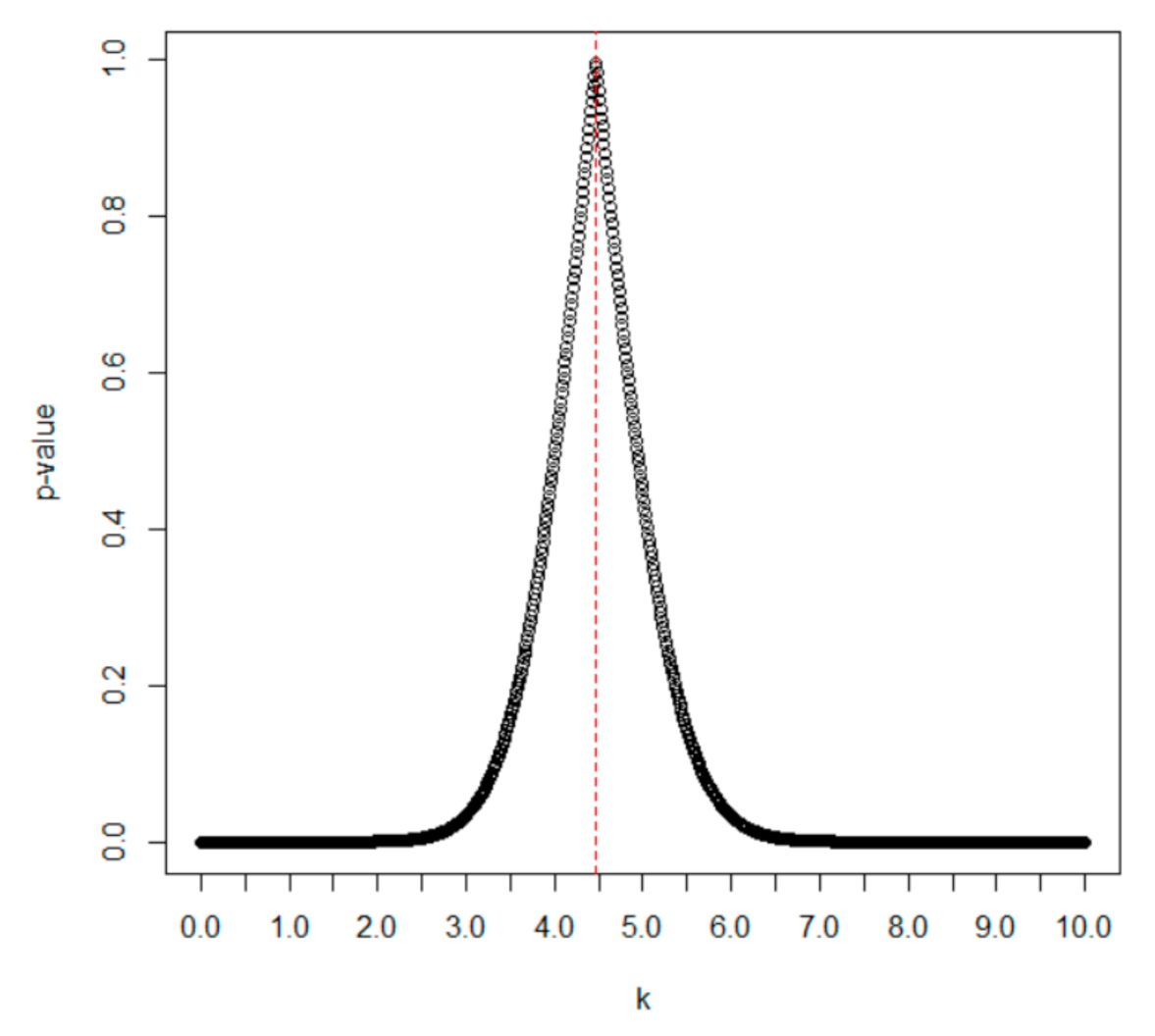
Using the Gini-test (see Gail and Gastwirth [13]), the Gini-test value , where . The Gini-test value is a function of k, and the p-values versus k values are plotted in Figure 7. We assume the parameter k is known. The value of k is determined with the the maximum p-value for Gini-test. It can be seen that the value of k is chosen as k = 4.47 with the maximum p-value.
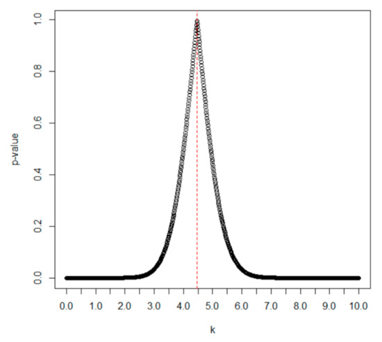
Figure 7.
The p-values for Gini test versus k values.
Referring to Section 3.1, suppose that the lower specification limit is L = 0.5, the number of inspection is m = 5, the removal probability is p = 0.05, the target lifetime performance index is c0 = 0.8, the level of significance is = 0.1, and the power is 1 − = 0.80 at c1 = 0.9. The required sample size is determined as n = 20 from Table 2.
Based on this setup, we can start to conduct the testing procedure about CL as follows:
Step 1: Take a random sample of size n = 20 from the data set. Observe the progressive type I interval censored sample (X1,X2,X3,X4,X5) = (0,0,1,7,2) at the pre-set times (t1,t2,t3,t4,t5) = (0.1,0.2,0.3,0.4,0.5) with censoring schemes of (R1,R2,R3,R4,R5) = (2,0,1,0,7) and (p1,p2, p3,p4,p5) = (0.05,0.05,0.05,0.05,1).
Step 2: Find the MLE of λ as = 0.4270091 and then obtain the test statistic = 1 − 0.4270091 × 0.05 = 0.9786495.
Step 3: For level of significance = 0.05, we can calculate the critical value = 0.8780724.
Step 4: Since = 0.9786495 > = 0.8780724, we should reject the null hypothesis and claim that the lifetime performance index of product meets the required level.
With respect to Section 3.2, m is not fixed and T = 0.5 is fixed, under the same consideration in the previous section except m and n are not determined. From Table 4, we can find that the optimal sampling design is m* = 3, n* = 21 with critical value = 0.8799 and resulting in the minimum total cost of 25.5 units under the cost setup of Co = 1 and a =b = c = 1.
We can start to conduct the testing procedure about as follows:
Step 1: Take a random sample of size n = 21 from the data set. Observe the progressive type I interval censored sample (X1,X2,X3) = (0,3,9) at the pre-set times (t1,t2,t3) = (0.1667,0.333,0.5) with censoring schemes of (R1,R2 R3) = (0,0,9) and (p1,p2,p3) = (0.05,0.05,1).
Step 2: Find the MLE of λ as = 0.4026597 and then obtain the test statistic = 1 − 0.4026597 × 0.05 = 0.979867.
Step 3: For level of significance = 0.05, we can calculate the critical value = 0.8799.
Step 4: Since = 0.979867 > = 0.8799, we conclude to reject the null hypothesis and claim that the lifetime performance index of product meets the required level.
With respect to Section 3.3, when m and t are not fixed under the same setup with the previous two cases, we can find that the optimal sampling design is m* = 3, n* = 21, and t* = 0.11 with critical value = 0.8783 and minimum total cost of 29.5 units under the cost setup of Co = 1 and a = b = c = 1 from Table 7.
The testing procedure about can be implemented as follows:
Step 1: Take a random sample of size n = 21 from the data set. Observe the progressive type I interval censored sample (X1,X2,X3) = (0,0,4) at the pre-set times (t1,t2,t3) = (0.11,0.22,0.33) with censoring schemes of (R1,R2,R3) = (1,2,14) and (p1,p2, p3) = (0.05,0.05,1).
Step 2: Find the MLE of λ as = 0.2921072 and then obtain the test statistic = 1 − 0.2921072 × 0.05 = 0.9853946.
Step 3: For level of significance = 0.05, we can calculate the critical value = 0.8783.
Step 4: Since = 0.9853946 > = 0.8783, we reached the same conclusion to support the alternative hypothesis.
4. Conclusions
For many practical cases, the collection of complete samples would be very costly or not be feasible. The progressive type I interval censoring is thus arisen. The progressive type-I interval censoring has the advantage of convenient collection of data for the quality personnel in the life test. For this type of censoring, we have developed a sampling design to determine the sample size for attaining the preassigned power for a level test or to determine the number of inspection intervals and interval lengths with the minimum total experimental cost for the test of the lifetime performance index CL when the lifetime of products is following the Gompertz distribution under two conditions. One condition is the consideration of fixed termination time of the experiment and the other condition is the consideration of unfixed termination time of the experiment. Our algorithms for the sampling design can help experimenters to setup the progressive type-I interval censoring scheme and to use the observed sample to conduct the hypothesis test to see if the lifetime performance index meets the desired target level. We have also given a real-life example to demonstrate our sampling design and the implementation on the hypothesis testing procedure regarding the lifetime performance index.
Author Contributions
Conceptualization, S.-F.W.; methodology, S.-F.W.; software, S.-F.W., Y.-J.X., M.-F.L. and W.-T.C.; validation, Y.-J.X., M.-F.L. and W.-T.C.; formal analysis, S.-F.W.; investigation, S.-F.W., Y.-J.X., M.-F.L. and W.-T.C.; resources, S.-F.W.; data curation, S.-F.W., Y.-J.X., M.-F.L. and W.-T.C.; writing—original draft preparation, S.-F.W. and W.-T.C.; writing—review and editing, S.-F.W.; visualization, Y.-J.X., M.-F.L. and W.-T.C.; supervision, S.-F.W.; project administration, S.-F.W.; funding acquisition, S.-F.W. All authors have read and agreed to the published version of the manuscript.
Funding
This research was funded by the Ministry of Science and Technology, Taiwan MOST 108-2118-M-032-001-and MOST 109-2118-M-032-001-MY2, and the APC was funded by MOST 109-2118-M-032-001-MY2.
Informed Consent Statement
Not applicable.
Data Availability Statement
Data available in a publicly accessible repository; the data presented in this study are openly available in Lee and Wang [12].
Conflicts of Interest
The authors declare no conflict of interest.
References
- Montgomery, D.C. Introduction to Statistical Quality Control; John Wiley and Sons Inc.: New York, NY, USA, 1985. [Google Scholar]
- Tong, L.I.; Chen, K.S.; Chen, H.T. Statistical testing for assessing the performance of lifetime index of electronic components with exponential distribution. Int. J. Qual. Reliab. Manag. 2002, 19, 812–824. [Google Scholar] [CrossRef]
- Balakrishnan, N.; Aggarwala, R. Progressive Censoring: Theory, Methods and Applications; Springer Science & Business Media: Boston, MA, USA, 2000. [Google Scholar]
- Aggarwala, R. Progressive interval censoring: Some mathematical results with applications to inference. Commun. Stat. Theory Methods 2001, 30, 1921–1935. [Google Scholar] [CrossRef]
- Lee, W.C.; Wu, J.W.; Hong, C.W. Assessing the lifetime performance index of products with the exponential distribution under progressively type II right censored samples. J. Comput. Appl. Math. 2009, 231, 648–656. [Google Scholar] [CrossRef] [Green Version]
- Wu, S.J.; Lin, Y.P.; Chen, Y.J. Planning step-stress life test with progressively type-I group-censored exponential data. Stat. Neerl. 2006, 60, 46–56. [Google Scholar] [CrossRef]
- Wu, S.J.; Lin, Y.P.; Chen, S.T. Optimal step-stress test under type I progressive group-censoring with random removals. J. Stat. Plan. Inference 2008, 138, 817–826. [Google Scholar] [CrossRef]
- Lee, H.M.; Wu, J.W.; Lei, C.L. Assessing the Lifetime Performance Index of Exponential Products with Step-Stress Accelerated Life-Testing Data. IEEE Trans. Reliab. 2013, 62, 296–304. [Google Scholar] [CrossRef]
- Wu, S.F.; Lin, Y.P. Computational testing algorithmic procedure of assessment for lifetime performance index of products with one-parameter exponential distribution under progressive type I interval censoring. Math. Comput. Simul. 2016, 120, 79–90. [Google Scholar] [CrossRef]
- Wu, S.F.; Hsieh, Y.T. The assessment on the lifetime performance index of products with Gompertz distribution based on the progressive type I interval censored sample. J. Comput. Appl. Math. 2019, 351, 66–76. [Google Scholar] [CrossRef]
- Huang, S.R.; Wu, S.J. Reliability sampling plans under progressive type-I interval censoring using cost functions. IEEE Trans. Reliab. 2008, 57, 445–451. [Google Scholar] [CrossRef]
- Lee, E.T.; Wang, J.W. Statistical Method for Survival Data Analysis; John Wiley & Sons, Inc.: New York, NY, USA, 2003. [Google Scholar]
- Gail, M.H.; Gastwirth, J.L. A scale-free goodness of fit test for the exponential distribution based on the Gini Statistic. J. R. Stat. Soc. B 1978, 40, 350–357. [Google Scholar] [CrossRef]
Publisher’s Note: MDPI stays neutral with regard to jurisdictional claims in published maps and institutional affiliations. |
© 2021 by the authors. Licensee MDPI, Basel, Switzerland. This article is an open access article distributed under the terms and conditions of the Creative Commons Attribution (CC BY) license (https://creativecommons.org/licenses/by/4.0/).