
Generalized Fractional Bézier Curve with Shape Parameters


Abstract
:1. Introduction
2. Generalized Fractional Bézier Basis Functions
2.1. Riemann-Liouville Fractional Integral
2.2. The Construction of Generalized Fractional Bézier Basis Function
- 1.
- Degeneracy: When and for , the basis function become classical Bernstein basis function.
- 2.
- Non-negativity: .
- 3.
- Partition of unity:
- 4.
- Symmetry: when and .
- 1.
- Degeneracy: When , and for implies . Hence, . Therefore, the basis functions becomes general Bernstein basis functions.
- 2.
- Non-negativity: For any and , it is clear that . Then, implies that . While, implies that . Hence, . Therefore, Equation (3) and implies that .
- 3.
- Partition of unity: Before the main proving, a lemma is proven first in order to prove the partition of unity.
- 4.
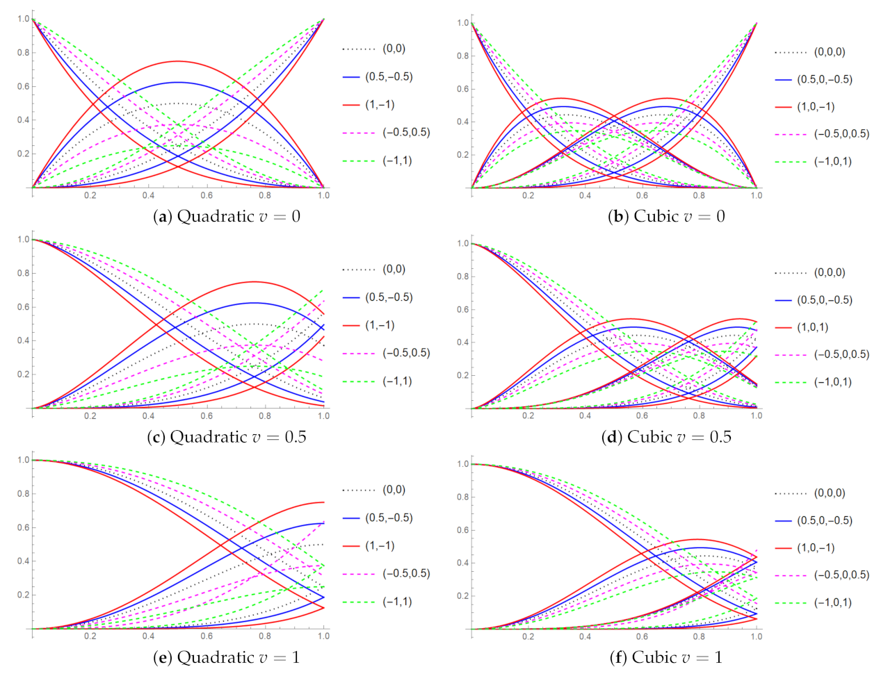
- Symmetry: Since and , the basis function become the Bernstein basis function; hence the symmetry properties is satisfied. Note that the symmetry properties will get a partial symmetrical shape when , but the curve still preserves the same feature of the symmetrical shape, on a different scale. Based on Figure 1 and Figure 2, it can be observed that the symmetry properties are in full shape when and . This new property is further discussed in Section 3.
3. Construction of Generalized Fractional Bézier Curve with Shape Parameters
3.1. Properties of Curve
- 1.
- Endpoint terminal
- 2.
- Endpoint tangent
- 3.
- Convex hull
- 4.
- Geometric invariance
- 5.
- Shape adjustable property
- 6.
- Fractional curve adjustable property
- 1.
- Endpoint terminal:For any value of and any degree of n, the endpoint terminal property is satisfied:For , the endpoint terminal will become the linear combination of , where . Note that when , then . At , the endpoint does not depend on the fractional parameter given in Equation (5). However, at , the endpoint is not fixed by its last control point as any normal Bézier curve. This implies that the endpoint for fractional Bézier curve at depends on the fractional parameter v. The coordinate of endpoint terminal can be obtained easily using Equation (5) by simply plugging in the value of fractional parameter v, where the specific coordinate of the endpoint at can be determined. This endpoint terminal property for the fractional Bézier curve will provide the particle path that is tractable when the value of v varies. Hence, the endpoint terminal property is satisfied.
- 2.
- Endpoint tangent:This endpoint tangent property is satisfied for . The values of the endpoint tangent are:For the endpoint tangent at , the tangent is not affected by fractional parameter v. Different values of v will determine the coordinate of the endpoint terminal for . Therefore, the endpoint tangent for depends on the value of v. By having this unique property of fractional parameter, the basis function will provide the optimal length of the curve so that the trajectory of the curve can be controlled. The desired length of the curve can be arbitrarily chosen when . Special case occur for endpoint at when , then the endpoint tangent . Hence, the endpoint tangent property is satisfied.
- 3.
- Convex hull:
- 4.
- Geometric invariance:Supposed is an arbitary vector in or and L is an arbitrary matrix with size for , then the following equation is satisfied:
- (a)
- (b)
- 5.
- Shape adjustable property:The classical Bézier curve is a fixed curve within the control polygon. The limitation of the classical Bézier curve is that the curve cannot be altered without changing the control points. The generalized fractional Bézier basis functions with shape parameters can overcome this limitation. The number of shape parameters constructed depends on the number of degrees. Here, the n-th degree of the curve will have n number of shape parameters. By using shape parameters, the curve is more flexible without changing the control points.
- 6.
- Fractional curve adjustable property:By applying the Riemann-Liouville fractional integral definition in the construction of the Bézier curve, a new parameter called fractional parameter is created. This fractional parameter is used for adjusting and controlling the length of the constructed curve. This property is further discussed in Section 3.3.
3.2. The Geometric Effect of Shape Parameter on the Curve
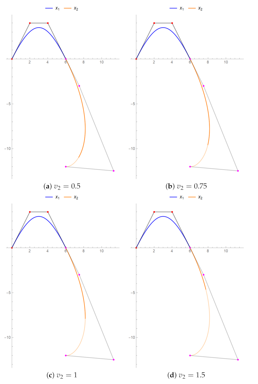
3.3. The Effect of Fractional Parameter on the Curve
3.4. Fractional De Casteljau Algorithm
3.5. Arc Length for Generalized Fractional Bézier Curve
4. Continuity for Generalized Fractional Bézier Curve
4.1. Parametric Continuity for Generalized Fractional Bézier Curve,
- 1.
- continuity:
- 2.
- continuity:
- 3.
- continuity:
- 1.
- Since is position continuity, hence common point of the two curves to connect should be decided. In this case, the endpoint of the first curve, , is connected to the first point of the second curve, . Hence, by solving , continuity condition will be satisfied.
- 2.
- continuity condition must be satisfied first. continuity is tangent continuity at the common point. By solving and , continuity condition of can be satisfied.
- 3.
- continuity is curvature continuity at the common point. By solving , , and , and conditions must be satisfied first in order for continuity to be satisfied.
4.2. Geometric Continuity for Generalized Fractional Bézier Curve,
- 1.
- continuity:
- 2.
- continuity:
- 3.
- continuity:
- 1.
- continuity is the position continuity same as continuity. By solving , continuity condition will be satisfied.
- 2.
- continuity is a tangent continuity at common point but with scale factor . By solving and with , continuity condition will only be satisfied when continuity is satisfied.
- 3.
- and continuity must be satisfied first. continuity is a curvature continuity at common point but with scale factors and . By solving , , and , with and , continuity condition will be satisfied.
4.3. Fractional Continuity for Generalized Fractional Bézier Curve,
- 1.
- continuity:
- 2.
- continuity:
- 3.
- continuity:
- 1
- continuity is the position continuity with fractional parameter . By solving , continuity condition will be satisfied.
- 2.
- continuity must be satisfied first. continuity is a tangent continuity at common point but with scale factor and fractional parameter . By solving and with , continuity condition will be satisfied.
- 3.
- and continuity must be satisfied first. continuity is a curvature continuity at common point but with scale factors and and fractional parameter . By solving , , and , with and , continuity condition will be satisfied.
- 1.
- continuity:
- 2.
- continuity:The control point for is the same as continuity condition.
- 3.
- continuity:The control point for and are the same as continuity condition.
5. Modelling of Shapes Using Generalized Fractional Bézier Curves
6. Construction of Surface Using Generalized Fractional Bézier Curve
6.1. Surface Revolution
6.2. Extruded Surface
7. Conclusions
Author Contributions
Funding
Acknowledgments
Conflicts of Interest
References
- Prautzsch, H.; Boehm, W.; Paluszny, M. Bézier and B-Spline Techniques; Springer Science & Business Media: Berlin/Heidelberg, Germany, 2002. [Google Scholar]
- Farin, G.E.; Farin, G. Curves and Surfaces for CAGD: A Practical Guide; Morgan Kaufmann: Burlington, MS, USA, 2002. [Google Scholar]
- Yang, L.; Zeng, X.M. Bézier curves and surfaces with shape parameters. Int. J. Comput. Math. 2009, 86, 1253–1263. [Google Scholar] [CrossRef]
- Wang, W.T.; Wang, G.Z. Bézier curves with shape parameter. J. Zhejiang Univ. Sci. A 2005, 6, 497–501. [Google Scholar]
- Dube, M.; Sharma, R. Quartic trignometric Bézier curve with a shape parameter. Int. J. Math. Comput. Appl. Res. 2013, 3, 89–96. [Google Scholar]
- Han, X.A.; Ma, Y.; Huang, X. The cubic trigonometric Bézier curve with two shape parameters. Appl. Math. Lett. 2009, 22, 226–231. [Google Scholar] [CrossRef] [Green Version]
- Misro, M.Y.; Ramli, A.; Ali, J.M. Quintic trigonometric Bézier curve with two shape parameters. Sains Malays. 2017, 46, 825–831. [Google Scholar]
- Misro, M.Y.; Ramli, A.; Ali, J.M.; Abd Hamid, N.N. Cubic trigonometric Bézier spiral curves. In Proceedings of the 2017 14th International Conference on Computer Graphics, Imaging and Visualization, Marrakesh, Morocco, 23–25 May 2017; pp. 14–20. [Google Scholar]
- Misro, M.Y.; Ramli, A.; Ali, J.M. Extended analysis of dynamic parameters on cubic trigonometric Bézier transition curves. In Proceedings of the 2019 23rd International Conference in Information Visualization–Part II, Paris, France, 2–5 July 2019; pp. 141–146. [Google Scholar]
- Misro, M.Y.; Ramli, A.; Ali, J.M.; Abd Hamid, N.N. Pythagorean hodograph quintic trigonometric Bézier transtion curve. In Proceedings of the 2017 14th International Conference on Computer Graphics, Imaging and Visualization, Marrakesh, Morocco, 23–25 May 2017; pp. 1–7. [Google Scholar]
- Misro, M.Y.; Ramli, A.; Ali, J.M. Quintic trigonometric Bézier curve and its maximum speed estimation on highway designs. In AIP Conference Proceedings; AIP Publishing LLC: Melville, NY, USA, 2018; p. 020089. [Google Scholar]
- Yan, Z.; Schiller, S.; Wilensky, G.; Carr, N.; Schaefer, S. K-curves: Interpolation at local maximum curvature. Acm Trans. Graph. (TOG) 2017, 36, 1–7. [Google Scholar] [CrossRef]
- Yuksel, C. A Class of C 2 Interpolating Splines. Acm Trans. Graph. (TOG) 2020, 39, 1–14. [Google Scholar] [CrossRef]
- Adnan, S.B.Z.; Ariffin, A.A.M.; Misro, M.Y. Curve fitting using quintic trigonometric Bézier curve. In AIP Conference Proceedings; AIP Publishing LLC: Melville, NY, USA, 2020; Volume 2266, p. 040009. [Google Scholar]
- Piegl, L.; Tiller, W. Curve and surface constructions using rational B-splines. Comput. Aided Des. 1987, 19, 485–498. [Google Scholar] [CrossRef]
- Dimas, E.; Briassoulis, D. 3D geometric modelling based on NURBS: A review. Adv. Eng. Softw. 1999, 30, 741–751. [Google Scholar] [CrossRef]
- Barbat, C.S. Examples of Bézier-Surfaces of Revolution. J. Geom. Graph. 2005, 9, 1–9. [Google Scholar]
- Ismail, N.H.M.; Misro, M.Y. Surface construction using continuous trigonometric Bézier curve. In AIP Conference Proceedings; AIP Publishing LLC: Melville, NY, USA, 2020; p. 040012. [Google Scholar]
- Ammad, M.; Misro, M.Y. Construction of Local Shape Adjustable Surfaces Using Quintic Trigonometric Bézier Curve. Symmetry 2020, 12, 1205. [Google Scholar] [CrossRef]
- DeRose, T.D.; Barsky, B.A. An intuitive approach to geometric continuity for parametric curves and surfaces. In Computer-Generated Images; Springer: Berlin/Heidelberg, Germany, 1985; pp. 159–175. [Google Scholar]
- Ziatdinov, R.; Yoshida, N.; Kim, T.w. Fitting G2 multispiral transition curve joining two straight lines. Comput. Aided Des. 2012, 44, 591–596. [Google Scholar] [CrossRef]
- Barsky, B.A.; DeRose, T.D. Geometric continuity of parametric curves: Constructions of geometrically continuous splines. IEEE Comput. Graph. Appl. 1990, 10, 60–68. [Google Scholar] [CrossRef]
- Qin, X.; Hu, G.; Zhang, N.; Shen, X.; Yang, Y. A novel extension to the polynomial basis functions describing Bézier curves and surfaces of degree n with multiple shape parameters. Appl. Math. Comput. 2013, 223, 1–16. [Google Scholar] [CrossRef]
- Bashir, U.; Abbas, M.; Ali, J.M. The G2 and C2 rational quadratic trigonometric Bézier curve with two shape parameters with applications. Appl. Math. Comput. 2013, 219, 10183–10197. [Google Scholar] [CrossRef]
- Hu, G.; Bo, C.; Qin, X. Continuity conditions for Q-Bézier curves of degree n. J. Inequal. Appl. 2017, 2017, 1–14. [Google Scholar] [CrossRef] [Green Version]
- BiBi, S.; Abbas, M.; Miura, K.T.; Misro, M.Y. Geometric Modeling of Novel Generalized Hybrid Trigonometric Bézier-Like Curve with Shape Parameters and Its Applications. Mathematics 2020, 8, 967. [Google Scholar] [CrossRef]
- Miller, K.S.; Ross, B. An Introduction to the Fractional Calculus and Fractional Differential Equations; Wiley: Hoboken, NJ, USA, 1993. [Google Scholar]
- Samko, S.G.; Kilbas, A.A.; Marichev, O.I. Fractional Integrals and Derivatives; Gordon and Breach Science Publishers: Yverdon Yverdon-les-Bains, Switzerland, 1993; Volume 1. [Google Scholar]
- Baleanu, D.; Güvenç, Z.B.; Machado, J.T. New Trends in Nanotechnology and Fractional Calculus Applications; Springer: Berlin/Heidelberg, Germany, 2010. [Google Scholar]
- Iqbal, S.; Mubeen, S.; Tomar, M. On Hadamard k-fractional integrals. J. Fract. Calc. Appl. 2018, 9, 255–267. [Google Scholar]
- Caputo, M. Linear models of dissipation whose Q is almost frequency independent—II. Geophys. J. Int. 1967, 13, 529–539. [Google Scholar] [CrossRef]
- Alqahtani, R.T. Atangana-Baleanu derivative with fractional order applied to the model of groundwater within an unconfined aquifer. J. Nonlinear Sci. Appl. 2016, 9, 3647–3654. [Google Scholar] [CrossRef] [Green Version]
- Li, X. Numerical solution of fractional differential equations using cubic B-spline wavelet collocation method. Commun. Nonlinear Sci. Numer. Simul. 2012, 17, 3934–3946. [Google Scholar] [CrossRef]
- Arshed, S. Quintic B-spline method for time-fractional superdiffusion fourth-order differential equation. Math. Sci. 2017, 11, 17–26. [Google Scholar] [CrossRef]
- Ghomanjani, F. A numerical technique for solving fractional optimal control problems and fractional Riccati differential equations. J. Egypt. Math. Soc. 2016, 24, 638–643. [Google Scholar] [CrossRef] [Green Version]
- Misro, M.Y.; Ramli, A.; Hoe, L.K. Determining degree of road elevation using spatial Bézier curve. In AIP Conference Proceedings; AIP Publishing LLC: Melville, NY, USA, 2019; Volume 2184, p. 060043. [Google Scholar]
- Barsky, B.A.; DeRose, T.D. Geometric continuity of parametric curves: Three equivalent characterizations. IEEE Comput. Graph. Appl. 1989, 9, 60–69. [Google Scholar] [CrossRef]


| Shape Parameters, | Fractional Parameter, v | Arc Length |
|---|---|---|
| (0, 0, 0) Black | 0 | 8.8737 |
| 0.25 | 7.4439 | |
| 0.5 | 6.1777 | |
| 1.5 | 3.1259 | |
| (0.75, 0.25, −0.8) Magenta | 0 | 9.4246 |
| 0.25 | 9.4064 | |
| 0.5 | 6.3326 | |
| 1.5 | 3.5155 | |
| (−0.6, −0.1, 0.9) Red | 0 | 8.3703 |
| 0.25 | 7.2651 | |
| 0.5 | 6.1023 | |
| 1.5 | 2.8168 |
Publisher’s Note: MDPI stays neutral with regard to jurisdictional claims in published maps and institutional affiliations. |
© 2021 by the authors. Licensee MDPI, Basel, Switzerland. This article is an open access article distributed under the terms and conditions of the Creative Commons Attribution (CC BY) license (https://creativecommons.org/licenses/by/4.0/).
Share and Cite
Said Mad Zain, S.A.A.A.; Misro, M.Y.; Miura, K.T. Generalized Fractional Bézier Curve with Shape Parameters. Mathematics 2021, 9, 2141. https://doi.org/10.3390/math9172141
Said Mad Zain SAAA, Misro MY, Miura KT. Generalized Fractional Bézier Curve with Shape Parameters. Mathematics. 2021; 9(17):2141. https://doi.org/10.3390/math9172141
Chicago/Turabian StyleSaid Mad Zain, Syed Ahmad Aidil Adha, Md Yushalify Misro, and Kenjiro T. Miura. 2021. "Generalized Fractional Bézier Curve with Shape Parameters" Mathematics 9, no. 17: 2141. https://doi.org/10.3390/math9172141